
Vector Embeddings
How to access and use Multilingual embedding models using OML for Python 2.1
With the release of OML for Python 2.1, we have a newer approach for accessing and generating embedding models in ONNX format (from Hugging Face), which can then be loaded into the Database (>=23.7ai). Although with this newer approach, we need to be aware of the previous way of doing it (<=23.6). As of 23.7ai this previous approach is now deprecated. Given the short time the previous approach was around, things could yet change with subsequent releases.
As the popularity of Vector Search spreads, there have been some challenges relating to obtaining and using suitable models within a Database. Oracle 23ai introduced the ability to load an embedding model in ONNX format into the database. These could be easily used to create and update embedding vectors for your data. But there were some limitations and challenges with what ONNX models could be used, and sometimes this was limited to the formatting of the ONNX metadata and the pretrained models themselves.
To ease the process of locating, converting and loading an embedding model into an Oracle Database, Oracle Machine Learning for Python 2.1 has been released with some new features and methods to make the process slightly easier. There are three constraints for doing this: 1) you need to use Oracle Machine Learning for Python 2.1 (OML4Py 2.1), and 2) you need to use Oracle 23.7ai (or greater) Database (This later requirement is to allow for the expanded range of embedding models) and 3) Python 3.12 (or greater).
There are a few additional Python libraries needed, so check the documentation for more details on what the most recent version of these should be. But do be careful of the documentation as the version I followed there was some inconsistencies in different sections regarding the requirements and steps to follow for installation. Hopefully this will be tidied up by the time you read the documentation.
With OML4Py 2.1 there is a class called oml.utils.onnxpipeline, with a number of methods to support the exploration of preconfigured models. These include: from_preconfigured(), from_template() and show_preconfigured(). This last one displays the list of preconfigured models.
oml.ONNXPipelineConfig.show_preconfigured()
['sentence-transformers/all-mpnet-base-v2', 'sentence-transformers/all-MiniLM-L6-v2', 'sentence-transformers/multi-qa-MiniLM-L6-cos-v1', 'sentence-transformers/distiluse-base-multilingual-cased-v2', 'sentence-transformers/all-MiniLM-L12-v2', 'BAAI/bge-small-en-v1.5', 'BAAI/bge-base-en-v1.5', 'taylorAI/bge-micro-v2', 'intfloat/e5-small-v2', 'intfloat/e5-base-v2', 'thenlper/gte-base', 'thenlper/gte-small', 'TaylorAI/gte-tiny', 'sentence-transformers/paraphrase-multilingual-mpnet-base-v2', 'intfloat/multilingual-e5-base', 'intfloat/multilingual-e5-small', 'sentence-transformers/stsb-xlm-r-multilingual', 'Snowflake/snowflake-arctic-embed-xs', 'Snowflake/snowflake-arctic-embed-s', 'Snowflake/snowflake-arctic-embed-m', 'mixedbread-ai/mxbai-embed-large-v1', 'openai/clip-vit-large-patch14', 'google/vit-base-patch16-224', 'microsoft/resnet-18', 'microsoft/resnet-50', 'WinKawaks/vit-tiny-patch16-224', 'Falconsai/nsfw_image_detection', 'WinKawaks/vit-small-patch16-224', 'nateraw/vit-age-classifier', 'rizvandwiki/gender-classification', 'AdamCodd/vit-base-nsfw-detector', 'trpakov/vit-face-expression', 'BAAI/bge-reranker-base']
We can inspect the full details of all models or for an individual model by changing some of the parameters.
oml.ONNXPipelineConfig.show_preconfigured(include_properties=True, model_name='microsoft/resnet-50')
[{'checksum': 'fca7567354d0cb0b7258a44810150f7c1abf8e955cff9320b043c0554ba81f8e', 'model_type': 'IMAGE_CONVNEXT', 'pre_processors_img': [{'name': 'DecodeImage', 'do_convert_rgb': True}, {'name': 'Resize', 'enable': True, 'size': {'height': 384, 'width': 384}, 'resample': 'bilinear'}, {'name': 'Rescale', 'enable': True, 'rescale_factor': 0.00392156862}, {'name': 'Normalize', 'enable': True, 'image_mean': 'IMAGENET_STANDARD_MEAN', 'image_std': 'IMAGENET_STANDARD_STD'}, {'name': 'OrderChannels', 'order': 'CHW'}], 'post_processors_img': []}]
Let’s prepare a preconfigured model using the simplest approach. In this example we’ll use the 'sentence-transformers/multi-qa-MiniLM-L6-cos-v1' model. Start by defining a pipeline.
pipeline = oml.utils.ONNXPipeline(model_name="sentence-transformers/multi-qa-MiniLM-L6-cos-v1")We now have the choice of loading it straight to your database using an already established OML connection.
pipeline.export2db("my_onnx_model_db")or you can export the model to a file
pipeline.export2file("my_onnx_model", output_dir="/home/oracle/onnx")
When you check the file system, you’ll see something like the following. Depending on the model you exported and any configuration changes to the model, the file size will vary in size.
-rw-r--r--. 1 oracle oracle 90636512 Apr 22 12:00 my_onnx_model.onnxIs you ran the export2file() function you’ll need to move that file to the database server. This will involve talking gently with the DBA to get their assistance. Once permission is obtained from the DBA, the ONNX file will be copied into a directory that is referenced from within the database. This is a simple task of defining an external file system directory where the file is located. In the example below the directory is referenced as ONNX_DIR. This is the reference defined in the database, which has a pointer to directory on the file system. The next task is to load the ONNX file into your Database schema.
BEGIN
   DBMS_VECTOR.LOAD_ONNX_MODEL(
        directory => 'ONNX_DIR',
        file_name => 'my_onnx_model.onnx',
        model_name => 'Multi-qa-MiniLM-L6-Cos-v1');
END;
Once loaded the model can be used to create Vector Embeddings.
Vector Databases – Part 3 – Vector Search
Searching semantic similarity in a data set is now equivalent to searching for nearest neighbors in a vector space instead of using traditional keyword searches using query predicates. The distance between “dog” and “wolf” in this vector space is shorter than the distance between “dog” and “kitten”. A “dog” is more similar to a “wolf” than it is to a “kitten”.

Vector data tends to be unevenly distributed and clustered into groups that are semantically related. Doing a similarity search based on a given query vector is equivalent to retrieving the K-nearest vectors to your query vector in your vector space.
Typically, you want to find an ordered list of vectors by ranking them, where the first row in the list is the closest or most similar vector to the query vector, the second row in the list is the second closest vector to the query vector, and so on. When doing a similarity search, the relative order of distances is what really matters rather than the actual distance.

Semantic search where the initial vector is the word “Puppy” and you want to identify the four closest words. Similarity searches tend to get data from one or more clusters depending on the value of the query vector, distance and the fetch size. Approximate searches using vector indexes can limit the searches to specific clusters, whereas exact searches visit vectors across all clusters.
Measuring distances in a vector space is the core of identifying the most relevant results for a given query vector. That process is very different from the well-known keyword filtering in the relational database world, which is very quick, simple and very very efficient. Vector distance functions involve more complicated computations.
There are several ways you can calculate distances to determine how similar, or dissimilar, two vectors are. Each distance metric is computed using different mathematical formulas. The time taken to calculate the distance between two vectors depends on many factors, including the distance metric used as well as the format of the vectors themselves, such as the number of vector dimensions and the vector dimension formats.
Generally, it’s best to match the distance metric you use to the one that was used to train the vector embedding model that generated the vectors. Common Distance metric functions include:
- Euclidean Distance
- Euclidean Distance Squared
- Cosine Similarity [most commonly used]
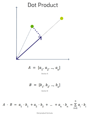
- Dot Product Similarity
- Manhattan Distance Hamming Similarity
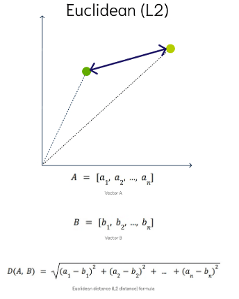
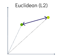
Euclidean Distance
This is a measure of the straight line distance between two points in the vector space. It ranges from 0 to infinity, where 0 represents identical vectors, and larger values represent increasingly dissimilar vectors. This is calculated using the Pythagorean theorem applied to the vector’s coordinates.
This metric is sensitive to both the vector’s size and it’s direction.
Euclidean Distance Squared
This is very similar to Euclidean Distance. When ordering is more important than the distance values themselves, the Squared Euclidean distance is very useful as it is faster to calculate than the Euclidean distance (avoiding the square-root calculation)
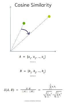
Cosine Similarity
This is the most commonly used distance measure. The cosine of the angle between two vectors – the larger the cosine, the closer the vectors. The smaller the angle, the bigger is its cosine. Cosine similarity measures the similarity in the direction or angle of the vectors, ignoring differences in their size (also called magnitude). The smaller the angle, the more similar are the two vectors. It ranges from -1 to 1, where 1 represents identical vectors, 0 represents orthogonal vectors, and -1 represents vectors that are diametrically opposed
DOT Product Similarity
DOT product similarity of two vectors can be viewed as multiplying the size of each vector by the cosine of their angle. The larger the dot product, the closer the vectors. You project one vector on the other and multiply the resulting vector sizes. Larger DOT product values imply that the vectors are more similar, while smaller values imply that they are less similar. It ranges from -∞ to ∞, where a positive value represents vectors that point in the same direction, 0 represents orthogonal vectors, and a negative value represents vectors that point in opposite directions
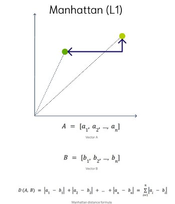
Manhattan Distance
This is calculated by summing the distance between the dimensions of the two vectors that you want to compare.
Imagine yourself in the streets of Manhattan trying to go from point A to point B. A straight line is not possible.
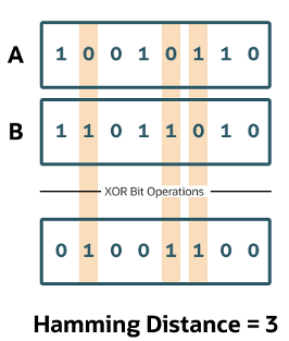
Hamming Similarity
This is the distance between two vectors represented by the number of dimensions where they differ. When using binary vectors, the Hamming distance between two vectors is the number of bits you must change to change one vector into the other. To compute the Hamming distance between two vectors, you need to compare the position of each bit in the sequence.
Check out my other posts in this series on Vector Databases.

You must be logged in to post a comment.