
Handling Multi-Column Indexes in Pandas Dataframes
It’s a little annoying when an API changes the structure of the data it returns and you end up with your code breaking. In my case, I experienced it when a dataframe having a single column index went to having a multi-column index. This was a new experience for me, at this time, as I hadn’t really come across it before. The following illustrates one particular case similar (not the same) that you might encounter. In this test/demo scenario I’ll be using the yfinance API to illustrate how you can remove the multi-column index and go back to having a single column index.
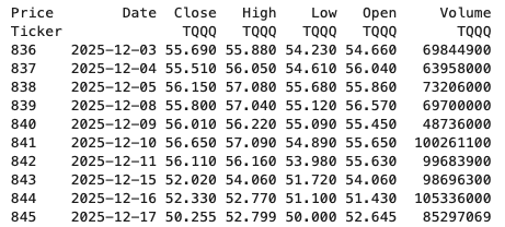
In this demo scenario, we are using yfinance to get data on various stocks. After the data is downloaded we get something like this.
The first step is to do some re-organisation.
df = data.stack(level="Ticker", future_stack=True)
df.index.names = ["Date", "Symbol"]
df = df[["Open", "High", "Low", "Close", "Volume"]]
df = df.swaplevel(0, 1)
df = df.sort_index()
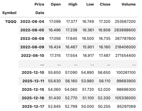
dfThis gives us the data in the following format.
The final part is to extract the data we want by applying a filter.
df.xs(“TQQQ”)
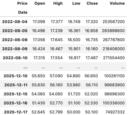
And there we have it.
As I said at the beginning the example above is just to illustrate what you can do.
If this was a real work example of using yfinance, I could just change a parameter setting in the download function, to not use multi_level_index.
data = yf.download(t, start=s_date, interval=time_interval, progress=False, multi_level_index=False)
Creating Test Data in your Database using Faker
A some point everyone needs some test data for their database. There area a number of ways of doing this, and in this post I’ll walk through using the Python library Faker to create some dummy test data (that kind of looks real) in my Oracle Database. I’ll have another post using the GenAI in-database feature available in the Oracle Autonomous Database. So keep an eye out for that.
Faker is one of the available libraries in Python for creating dummy/test data that kind of looks realistic. There are several more. I’m not going to get into the relative advantages and disadvantages of each, so I’ll leave that task to yourself. I’m just going to give you a quick demonstration of what is possible.
One of the key elements of using Faker is that we can set a geograpic location for the data to be generated. We can also set multiples of these and by setting this we can get data generated specific for that/those particular geographic locations. This is useful for when testing applications for different potential markets. In my example below I’m setting my local for USA (en_US).
Here’s the Python code to generate the Test Data with 15,000 records, which I also save to a CSV file.
import pandas as pd
from faker import Faker
import random
from datetime import date, timedelta

#####################
NUM_RECORDS = 15000
LOCALE = 'en_US'

#Initialise Faker
Faker.seed(42)
fake = Faker(LOCALE)

#####################

#Create a function to generate the data
def create_customer_record():
    #Customer Gender
    gender = random.choice(['Male', 'Female', 'Non-Binary'])
    #Customer Name
    if gender == 'Male':
        name = fake.name_male()
    elif gender == 'Female':
        name = fake.name_female()
    else:
        name = fake.name()

    #Date of Birth
    dob = fake.date_of_birth(minimum_age=18, maximum_age=90)

    #Customer Address and other details
    address = fake.street_address()
    email = fake.email()
    city = fake.city()
    state = fake.state_abbr()
    zip_code = fake.postcode()
    full_address = f"{address}, {city}, {state} {zip_code}"
    phone_number = fake.phone_number()

    #Customer Income
    #  - annual income between $30,000 and $250,000
    income = random.randint(300, 2500) * 100

    #Credit Rating
    credit_rating = random.choices(['A', 'B', 'C', 'D'], weights=[0.40, 0.30, 0.20, 0.10], k=1)[0]

    #Credit Card and Banking details
    card_type = random.choice(['visa', 'mastercard', 'amex'])
    credit_card_number = fake.credit_card_number(card_type=card_type)
    routing_number = fake.aba()
    bank_account = fake.bban()

    return {
        'CUSTOMERID': fake.unique.uuid4(), # Unique identifier
        'CUSTOMERNAME': name,
        'GENDER': gender,
        'EMAIL': email,
        'DATEOFBIRTH': dob.strftime('%Y-%m-%d'),
        'ANNUALINCOME': income,
        'CREDITRATING': credit_rating,
        'CUSTOMERADDRESS': full_address,
        'ZIPCODE': zip_code,
        'PHONENUMBER': phone_number,
        'CREDITCARDTYPE': card_type.capitalize(),
        'CREDITCARDNUMBER': credit_card_number,
        'BANKACCOUNTNUMBER': bank_account,
        'ROUTINGNUMBER': routing_number,
    }

#Generate the Demo Data
print(f"Generating {NUM_RECORDS} customer records...")
data = [create_customer_record() for _ in range(NUM_RECORDS)]
print("Sample Data Generation complete")

#Convert to Pandas DataFrame
df = pd.DataFrame(data)

print("\n--- DataFrame Sample (First 10 Rows) : sample of columns ---")
# Display relevant columns for verification
display_cols = ['CUSTOMERNAME', 'GENDER', 'DATEOFBIRTH', 'PHONENUMBER', 'CREDITCARDNUMBER', 'CREDITRATING', 'ZIPCODE']
print(df[display_cols].head(10).to_markdown(index=False))

print("\n--- DataFrame Information ---")
print(f"Total Rows: {len(df)}")
print(f"Total Columns: {len(df.columns)}")
print("Data Types:")
print(df.dtypes)
The output from the above code gives the following:
Generating 15000 customer records...
Sample Data Generation complete

--- DataFrame Sample (First 10 Rows) : sample of columns ---
| CUSTOMERNAME     | GENDER     | DATEOFBIRTH   | PHONENUMBER            |   CREDITCARDNUMBER | CREDITRATING   |   ZIPCODE |
|:-----------------|:-----------|:--------------|:-----------------------|-------------------:|:---------------|----------:|
| Allison Hill     | Non-Binary | 1951-03-02    | 479.540.2654           |   2271161559407810 | A              |     55488 |
| Mark Ferguson    | Non-Binary | 1952-09-28    | 724.523.8849x696       |    348710122691665 | A              |     84760 |
| Kimberly Osborne | Female     | 1973-08-02    | 001-822-778-2489x63834 |   4871331509839301 | B              |     70323 |
| Amy Valdez       | Female     | 1982-01-16    | +1-880-213-2677x3602   |   4474687234309808 | B              |     07131 |
| Eugene Green     | Male       | 1983-10-05    | (442)678-4980x841      |   4182449353487409 | A              |     32519 |
| Timothy Stanton  | Non-Binary | 1937-10-13    | (707)633-7543x3036     |    344586850142947 | A              |     14669 |
| Eric Parker      | Male       | 1964-09-06    | 577-673-8721x48951     |   2243200379176935 | C              |     86314 |
| Lisa Ball        | Non-Binary | 1971-09-20    | 516.865.8760           |    379096705466887 | A              |     93092 |
| Garrett Gibson   | Male       | 1959-07-05    | 001-437-645-2991       |    349049663193149 | A              |     15494 |
| John Petersen    | Male       | 1978-02-14    | 367.683.7770           |   2246349578856859 | A              |     11722 |

--- DataFrame Information ---
Total Rows: 15000
Total Columns: 14
Data Types:
CUSTOMERID           object
CUSTOMERNAME         object
GENDER               object
EMAIL                object
DATEOFBIRTH          object
ANNUALINCOME          int64
CREDITRATING         object
CUSTOMERADDRESS      object
ZIPCODE              object
PHONENUMBER          object
CREDITCARDTYPE       object
CREDITCARDNUMBER     object
BANKACCOUNTNUMBER    object
ROUTINGNUMBER        object
Having generated the Test data, we now need to get it into the database. There a various ways of doing this. As we are already using Python I’ll illustrate getting the data into the Database below. An alternative option is to use SQL Command Line (SQLcl) and the LOAD feature in that tool.
Here’s the Python code to load the data. I’m using the oracledb python library.
### Connect to Database
import oracledb

p_username = "..."
p_password = "..."

#Give OCI Wallet location and details
try:
    con = oracledb.connect(user=p_username, password=p_password, dsn="adb26ai_high",
                       config_dir="/Users/brendan.tierney/Dropbox/Wallet_ADB26ai",
                       wallet_location="/Users/brendan.tierney/Dropbox/Wallet_ADB26ai",
                       wallet_password=p_walletpass)
except Exception as e:
    print('Error connecting to the Database')
    print(f'Error:{e}')

print(con)
### Create Customer Table
drop_table = 'DROP TABLE IF EXISTS demo_customer'
cre_table = '''CREATE TABLE DEMO_CUSTOMER (
CustomerID VARCHAR2(50) PRIMARY KEY,
CustomerName VARCHAR2(50),
Gender VARCHAR2(10),
Email VARCHAR2(50),
DateOfBirth DATE,
AnnualIncome NUMBER(10,2),
CreditRating VARCHAR2(1),
CustomerAddress VARCHAR2(100),
ZipCode VARCHAR2(10),
PhoneNumber VARCHAR2(50),
CreditCardType VARCHAR2(10),
CreditCardNumber VARCHAR2(30),
BankAccountNumber VARCHAR2(30),
RoutingNumber VARCHAR2(10) )'''
cur = con.cursor()
print('--- Dropping DEMO_CUSTOMER table ---')
cur.execute(drop_table)
print('--- Creating DEMO_CUSTOMER table ---')
cur.execute(cre_table)
print('--- Table Created ---')### Insert Data into Table
insert_data = '''INSERT INTO DEMO_CUSTOMER values (:1, :2, :3, :4, :5, :6, :7, :8, :9, :10, :11, :12, :13, :14)'''
print("--- Inserting records ---")
cur.executemany(insert_data, df )
con.commit()
print("--- Saving to CSV ---")
df.to_csv('/Users/brendan.tierney/Dropbox/DEMO_Customer_data.csv', index=False)
print("- Finished -")### Close Connections to DB
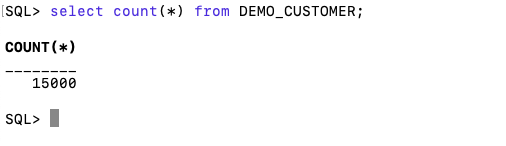
con.close()and to prove the records got inserted we can connect to the schema using SQLcl and check.
What a difference a Bind Variable makes
To bind or not to bind, that is the question?
Over the years, I heard and read about using Bind variables and how important they are, particularly when it comes to the efficient execution of queries. By using bind variables, the optimizer will reuse the execution plan from the cache rather than generating it each time. Recently, I had conversations about this with a couple of different groups, and they didn’t really believe me and they asked me to put together a demonstration. One group said they never heard of ‘prepared statements’, ‘bind variables’, ‘parameterised query’, etc., which was a little surprising.
The following is a subset of what I demonstrated to them to illustrate the benefits and potential benefits.
Here is a basic example of a typical scenario where we have a SQL query being constructed using concatenation.
select * from order_demo where order_id = || 'i';That statement looks simple and harmless. When we try to check the EXPLAIN plan from the optimizer we will get an error, so let’s just replace it with a number, because that’s what the query will end up being like.
select * from order_demo where order_id = 1;When we check the Explain Plan, we get the following. It looks like a good execution plan as it is using the index and then doing a ROWID lookup on the table. The developers were happy, and that’s what those recent conversations were about and what they are missing.
-------------------------------------------------------------
| Id  | Operation                   | Name         | E-Rows |
-------------------------------------------------------------
|   0 | SELECT STATEMENT            |              |        |
|   1 |  TABLE ACCESS BY INDEX ROWID| ORDER_DEMO   |      1 |
|*  2 |   INDEX UNIQUE SCAN         | SYS_C0014610 |      1 |
-------------------------------------------------------------
The missing part in their understanding was what happens every time they run their query. The Explain Plan looks good, so what’s the problem? The problem lies with the Optimizer evaluating the execution plan every time the query is issued. But the developers came back with the idea that this won’t happen because the execution plan is cached and will be reused. The problem with this is how we can test this, and what is the alternative, in this case, using bind variables (which was my suggestion).
Let’s setup a simple test to see what happens. Here is a simple piece of PL/SQL code which will look 100K times to retrieve just one row. This is very similar to what they were running.
DECLARE
   start_time TIMESTAMP;
   end_time   TIMESTAMP;
BEGIN
   start_time := systimestamp;
   dbms_output.put_line('Start time : ' || to_char(start_time,'HH24:MI:SS:FF4'));
   --
   for i in 1 .. 100000 loop
      execute immediate 'select * from order_demo where order_id = '||i;
   end loop;
   --
   end_time := systimestamp;
   dbms_output.put_line('End time : ' || to_char(end_time,'HH24:MI:SS:FF4'));
END;
/
When we run this test against a 23.7 Oracle Database running in a VM on my laptop, this completes in little over 2 minutes
Start time : 16:26:04:5527
End time : 16:28:13:4820


PL/SQL procedure successfully completed.

Elapsed: 00:02:09.158
The developers seemed happy with that time! Ok, but let’s test it using bind variables and see if it’s any different. There are a few different ways of setting up bind variables. The PL/SQL code below is one example.
DECLARE
   order_rec  ORDER_DEMO%rowtype;
   start_time TIMESTAMP;
   end_time   TIMESTAMP;
BEGIN
   start_time := systimestamp;
   dbms_output.put_line('Start time : ' || to_char(start_time,'HH24:MI:SS:FF9'));
   --
   for i in 1 .. 100000 loop
   execute immediate 'select * from order_demo where order_id = :1' using i;
	end loop;
	--
    end_time := systimestamp;
    dbms_output.put_line('End time : ' || to_char(end_time,'HH24:MI:SS:FF9'));
END;
/
Start time : 16:31:39:162619000
End time : 16:31:40:479301000


PL/SQL procedure successfully completed.

Elapsed: 00:00:01.363
This just took a little over one second to complete. Let me say that again, a little over one second to complete. We went from taking just over two minutes to run, down to just over one second to run.
The developers were a little surprised or more correctly, were a little shocked. But they then said the problem with that demonstration is that it is running directly in the Database. It will be different running it in Python across the network.
Ok, let me set up the same/similar demonstration using Python. The image below show some back Python code to connect to the database, list the tables in the schema and to create the test table for our demonstration

The first demonstration is to measure the timing for 100K records using the concatenation approach. I
# Demo - The SLOW way - concat values
#print start-time
print('Start time: ' + datetime.now().strftime("%H:%M:%S:%f"))

# only loop 10,000 instead of 100,000 - impact of network latency
for i in range(1, 100000):
    cursor.execute("select * from order_demo where order_id = " + str(i))

#print end-time
print('End time: ' + datetime.now().strftime("%H:%M:%S:%f"))
----------
Start time: 16:45:29:523020
End time: 16:49:15:610094
This took just under four minutes to complete. With PL/SQL it took approx two minutes. The extrat time is due to the back and forth nature of the client-server communications between the Python code and the Database. The developers were a little unhappen with this result.
The next step for the demonstrataion was to use bind variables. As with most languages there are a number of different ways to write and format these. Below is one example, but some of the others were also tried and give the same timing.
#Bind variables example - by name

#print start-time
print('Start time: ' + datetime.now().strftime("%H:%M:%S:%f"))

for i in range(1, 100000):
    cursor.execute("select * from order_demo where order_id = :order_num", order_num=i )

#print end-time
print('End time: ' + datetime.now().strftime("%H:%M:%S:%f"))
----------
Start time: 16:53:00:479468
End time: 16:54:14:197552
This took 1 minute 14 seconds. [Read that sentence again]. Compared to approx four minutes, and yes the other bind variable options has similar timing.
To answer the quote at the top of this post, “To bind or not to bind, that is the question?”, the answer is using Bind Variables, Prepared Statements, Parameterised Query, etc will make you queries and applications run a lot quicker. The optimizer will see the structure of the query, will see the parameterised parts of it, will see the execution plan already exists in the cache and will use it instead of generating the execution plan again. Thereby saving time for frequently executed queries which might just have a different value for one or two parts of a WHERE clause.
Comparing Text using Soundex, PHONIC_ENCODE and FUZZY_MATCH
When comparing text strings we have a number of functions on Oracle Database to help us. These include SOUNDEX, PHONIC_ENCODE and FUZZY_MATCH. Let’s have a look at what each of these can do.
The SOUNDEX function returns a character string containing the phonetic representation of a string. SOUNDEX lets you compare words that are spelled differently, but sound alike in English. To illustrate this, let’s compare some commonly spelled words and their variations, for example McDonald, MacDonald, and Smith and Smyth.
select soundex('MCDONALD') from dual;

SOUNDEX('MCDONALD')
___________________
M235

SQL> select soundex('MACDONALD') from dual;

SOUNDEX('MACDONALD')
____________________
M235

SQL> pause  next_smith_smyth
 next_smith_smyth


SQL>
SQL> select soundex('SMITH') from dual;

SOUNDEX('SMITH')
________________
S530

SQL> select soundex('SMYTH') from dual;

SOUNDEX('SMYTH')
________________
S530
Here we get to see SOUNDEX function returns the same code for each of the spelling variations. This function can be easily used to search for and to compare text in our tables.
Now let’s have a look at some of the different ways to spell Brendan.
select soundex('Brendan'),
  2         soundex('BRENDAN'),
  3  	   soundex('Breandan'),
  4  	   soundex('Brenden'),
  5  	   soundex('Brandon'),
  6  	   soundex('Brendawn'),
  7  	   soundex('Bhenden'),
  8  	   soundex('Brendin'),
  9  	   soundex('Brendon'),
 10  	   soundex('Beenden'),
 11  	   soundex('Breenden'),
 12  	   soundex('Brendin'),
 13  	   soundex('Brendyn'),
 14  	   soundex('Brandon'),
 15  	   soundex('Brenainn'),
 16  	   soundex('Bréanainn')
 17  from dual;

SOUNDEX('BRENDAN') SOUNDEX('BRENDAN') SOUNDEX('BREANDAN') SOUNDEX('BRENDEN') SOUNDEX('BRANDON') SOUNDEX('BRENDAWN') SOUNDEX('BHENDEN') SOUNDEX('BRENDIN') SOUNDEX('BRENDON') SOUNDEX('BEENDEN') SOUNDEX('BREENDEN') SOUNDEX('BRENDIN') SOUNDEX('BRENDYN') SOUNDEX('BRANDON') SOUNDEX('BRENAINN') SOUNDEX('BRÉANAINN')
__________________ __________________ ___________________ __________________ __________________ ___________________ __________________ __________________ __________________ __________________ ___________________ __________________ __________________ __________________ ___________________ ____________________
B653               B653               B653                B653               B653               B653                B535               B653               B653               B535               B653                B653               B653               B653               B655                B655
We can see which variations of my name can be labeled as being similar in sound.
An alternative function is to use the PHONIC_ENCODE. The PHONIC_ENCODE function converts text into language-specific codes based on the pronunciation of the text. It implements the Double Metaphone algorithm and an alternative algorithm. DOUBLE_METAPHONE returns the primary code. DOUBLE_METAPHONE_ALT returns the alternative code if present. If the alternative code is not present, it returns the primary code.
select col, phonic_encode(double_metaphone,col) double_met
  2  from ( values
  3  	    ('Brendan'), ('BRENDAN'), ('Breandan'), ('Brenden'), ('Brandon'),
  4  		('Brendawn'), ('Bhenden'), ('Brendin'), ('Brendon'), ('Beenden'),
  5  		('Breenden'), ('Brendin'), ('Brendyn'), ('Brandon'), ('Brenainn'),
  6  		('Bréanainn')
  7       ) names (col);

COL       DOUBLE_MET
_________ __________
Brendan   PRNT
BRENDAN   PRNT
Breandan  PRNT
Brenden   PRNT
Brandon   PRNT
Brendawn  PRNT
Bhenden   PNTN
Brendin   PRNT
Brendon   PRNT
Beenden   PNTN
Breenden  PRNT
Brendin   PRNT
Brendyn   PRNT
Brandon   PRNT
Brenainn  PRNN
Bréanainn PRNN
The final function we’ll look at is FUZZY_MATCH. The FUZZY_MATCH function is language-neutral. It determines the similarity between two strings and supports several algorithms. Here is a simple example, again using variations of Brendan
with names (col) as (
  2      values
  3      ('Brendan'), ('BRENDAN'), ('Breandan'), ('Brenden'), ('Brandon'),
  4  	('Brendawn'), ('Bhenden'), ('Brendin'), ('Brendon'), ('Beenden'),
  5  	('Breenden'), ('Brendin'), ('Brendyn'), ('Brandon'), ('Brenainn'),
  6  	('Bréanainn') )
  7  select a.col, b.col, fuzzy_match(levenshtein, a.col, b.col) as lev
  8  from names a, names b
  9  where a.col != b.col;

COL      COL       LEV
________ _________ ___
Brendan  BRENDAN    15
Brendan  Breandan   88
Brendan  Brenden    86
Brendan  Brandon    72
Brendan  Brendawn   88
Brendan  Bhenden    72
Brendan  Brendin    86
Brendan  Brendon    86
Brendan  Beenden    72
Brendan  Breenden   75
Brendan  Brendin    86
Brendan  Brendyn    86
Brendan  Brandon    72
Brendan  Brenainn   63
Brendan  Bréanainn  45
...
Only a portion of the output is shown above. Similar solution would be the following and additionally we can compare the outputs from a number of the algorithms.
with names (col) as (
      values
      ('Brendan'), ('BRENDAN'), ('Breandan'), ('Brenden'), ('Brandon'),
  	('Brendawn'), ('Bhenden'), ('Brendin'), ('Brendon'), ('Beenden'),
  	('Breenden'), ('Brendin'), ('Brendyn'), ('Brandon'), ('Brenainn'),
  	('Bréanainn') )
  select a.col as col1, b.col as col2,
         fuzzy_match(levenshtein, a.col, b.col) as lev,
         fuzzy_match(jaro_winkler, a.col, b.col) as jaro_winkler,
         fuzzy_match(bigram, a.col, b.col) as bigram,
         fuzzy_match(trigram, a.col, b.col) as trigram,
         fuzzy_match(whole_word_match, a.col, b.col) as jwhole_word,
         fuzzy_match(longest_common_substring, a.col, b.col) as lcs
  from names a, names b
  where a.col != b.col
  and ROWNUM <= 10;

COL1    COL2     LEV JARO_WINKLER BIGRAM TRIGRAM JWHOLE_WORD LCS
_______ ________ ___ ____________ ______ _______ ___________ ___
Brendan BRENDAN   15           48      0       0           0  14
Brendan Breandan  88           93     71      50           0  50
Brendan Brenden   86           94     66      60           0  71
Brendan Brandon   72           84     50       0           0  28
Brendan Brendawn  88           97     71      66           0  75
Brendan Bhenden   72           82     33      20           0  42
Brendan Brendin   86           94     66      60           0  71
Brendan Brendon   86           94     66      60           0  71
Brendan Beenden   72           82     33      20           0  42
Brendan Breenden  75           90     57      33           0  37
By default, the output is a percentage similarity, but the UNSCALED keyword can be added to return the raw value.
with names (col) as (
      values
      ('Brendan'), ('BRENDAN'), ('Breandan'), ('Brenden'), ('Brandon'),
  	('Brendawn'), ('Bhenden'), ('Brendin'), ('Brendon'), ('Beenden'),
  	('Breenden'), ('Brendin'), ('Brendyn'), ('Brandon'), ('Brenainn'),
  	('Bréanainn') )
  select a.col as col1, b.col as col2,
         fuzzy_match(levenshtein, a.col, b.col, unscaled) as lev,
         fuzzy_match(jaro_winkler, a.col, b.col, unscaled) as jaro_winkler,
         fuzzy_match(bigram, a.col, b.col, unscaled) as bigram,
         fuzzy_match(trigram, a.col, b.col, unscaled) as trigram,
         fuzzy_match(whole_word_match, a.col, b.col, unscaled) as jwhole_word,
         fuzzy_match(longest_common_substring, a.col, b.col, unscaled) as lcs
  from names a, names b
  where a.col != b.col
  and ROWNUM <= 10;

COL1    COL2     LEV JARO_WINKLER BIGRAM TRIGRAM JWHOLE_WORD LCS
_______ ________ ___ ____________ ______ _______ ___________ ___
Brendan BRENDAN    6         0.48      0       0           0   1
Brendan Breandan   1         0.93      5       3           0   4
Brendan Brenden    1         0.94      4       3           0   5
Brendan Brandon    2         0.84      3       0           0   2
Brendan Brendawn   1         0.97      5       4           0   6
Brendan Bhenden    2         0.82      2       1           0   3
Brendan Brendin    1         0.94      4       3           0   5
Brendan Brendon    1         0.94      4       3           0   5
Brendan Beenden    2         0.82      2       1           0   3
Brendan Breenden   2          0.9      4       2           0   3
This was another post in the ‘Back to Basics’ series of posts. Make sure to check out the other posts in the series.
SQL Firewall – Part 2
In a previous post, we’ve explored some of the core functionality of SQL Firewall in Oracle 23ai, In this post I’ll explore some of the other functionality that I’ve had to use as we’ve deployed SQL Firewall over the past few weeks.
Sometimes, when querying the DBA_SQL_FIREWALL_VIOLATIONS view, you might not get the current up to-date violations, or if you are running it for the first time you might get now rows or violations being returned from the view. This is a slight timing issue, as the violations log/cacbe might not have been persisted to the data dictionary. If you end up in this kind of situation you might need to flush the logs to to data dictionary. To do this, run the following.
exec dbms_sql_firewall.flush_logs;As you work with SQL Firewall on an ongoing basis, where you are turning it on and off at various stages, it can be easy to lose track of whether the Firewall is turned on or off. Being able to check the current status becomes important. To check the currect status, we can query DBA_SQL_FIREWALL_STATUS
select status
from dba_sql_firewall_status;
STATUS
——–
ENABLED
After checking that, we can then run either of the following.
exec dbms_sql_firewall.disable;or
exec dbms_sql_firewall.enableAfter creating your Allowed Lists for your various scenarios, at some point, you might need to add or remove individual statements/queries from a list. An important element for this is to locate the SQL_ID and SQL_SIGNATURE.
exec dbsm_sql_firewall.delete_allowed_sql(username => 'SCOTT', allowed_sql_id => 1);and to add a single statement
exec dbms_sql_firewall.append_allow_list_single_sql(username => 'SCOTT', sql_signature  => '... ... ... ...',
    current_user   => 'PSMITH', top_level      => 'Y',
    source         => DBMS_SQL_FIREWALL.VIOLATION_LOG);
If you are using the Database Scheduler to run jobs, these will keep appearing in the Firewall logs. As these jobs run on a regular basis and new jobs can be added all the time, you will need to manage these. An alternative is to assume these jobs are safe to run. With SQL Firewall the managing of these can be very easy by getting SQL Firewall to ignore them.
exec dbms_sql_firewall.execlude(DBMS_SQL_FIREWALL.SCHEDULAR_JOB);SQL Firewall – Part 1
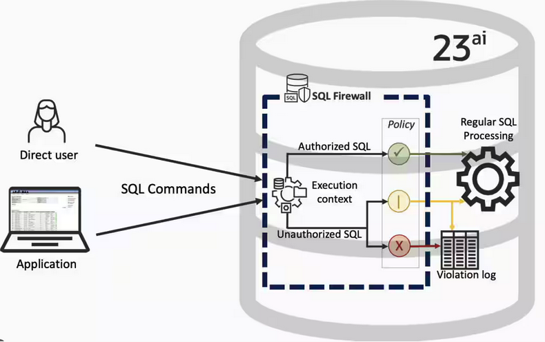
Typically, most IT architectures involve a firewall to act as a barrier, to monitor and to control network traffic. Its aim is to prevent unauthorised access and malicious activity. The firewall enforces rules to allow or block specific traffic (and commands/code). The firewall tries to protect our infrastructure and data. Over time, we have seen examples of how such firewalls have failed. We’ve also seen how our data (and databases) can be attacked internally. There are many ways to access the data and database without using the application. Many different people can have access to the data/database for many different purposes. There has been a growing need to push the idea of and the work of the firewall back to being closer to the data, that is, into the database.
SQL Firewall allows you to implement a firewall within the database to control what commands are allowed to be run on the data. With SQL Firewall you can:
- Monitor the SQL (and PL/SQL) activity to learn what the normal or typical SQL commands are being run on the data
- Captures all commands and logs them
- Manage a list of allowed commands, etc, using Policies
- Block and log all commands that are not allowed. Some commands might be allowed to run
Let’s walk through a simple example of setting this up and using it. For this example I’m assuming you have access to SYSTEM and another schema, for example SCOTT schema with the EMP, DEPT, etc tables.
Step 1 involves enabling SQL Firewall. To do this, we need to connect to the SYS schema and run the function to enable it.
grant sql_firewall_admin to system;Then connect to SYSTEM to enable the firewall.
exec dbms_sql_firewall.enable;For Step 2 we need to turn it on, as in we want to capture some of the commands being performed on the Database. We are using the SCOTT schema, so let’s capture what commands are run in that schema. [remember we are still connected to SYSTEM schema]
begin
  dbms_sql_firewall.create_capture (
    username=>'SCOTT',
    top_level_only=>true);
end;
Now that SQL Firewall is running, Step 3, we can switch to and connect to the SCOTT schema. When logged into SCOTT we can run some SQL commands on our tables.
select * from dept;
select deptno, count(*) from emp group by deptno;
select * from emp where job = 'MANAGER';
For Step 4, we can log back into SYSTEM and stop the capture of commands.
exec dbms_sql_firewall.stop_capture('SCOTT');We can then use the dictionary view DBA_SQL_FIREWALL_CAPTURE_LOG to see what commands were captured and logged.
column command_type format a12
column current_user format a15
column client_program format a45
column os_user format a10
column ip_address format a10
column sql_text format a30

select command_type,
       current_user,
       client_program,
       os_user,
       ip_address,
       sql_text
from   dba_sql_firewall_capture_logs
where  username = 'SCOTT';
The screen isn’t wide enough to display the results, but if you run the above command, you’ll see the three SELECT commands we ran above.
Other SQL Firewall dictionary views include DBA_SQL_FIREWALL_ALLOWED_IP_ADDR, DBA_SQL_FIREWALL_ALLOWED_OS_PROG, DBA_SQL_FIREWALL_ALLOWED_OS_USER and DBA_SQL_FIREWALL_ALLOWED_SQL.
For Step 5, we want to say that those commands are the only commands allowed in the SCOTT schema. We need to create an allowed list. Individual commands can be added, or if we want to add all the commands captured in our log, we can simple run
exec dbms_sql_firewall.generate_allow_list ('SCOTT');
exec  dbms_sql_firewall.enable_allow_list (username=>'SCOTT',block=>true);
Step 6 involves testing to see if the generated allowed list for SQL Firewall work. For this we need to log back into SCOTT schema, and run some commands. Let’s start with the three previously run commands. These should run without any problems or errors.
select * from dept;
select deptno, count(*) from emp group by deptno;
select * from emp where job = 'MANAGER';
Now write a different query and see what is returned.
select count(*) from dept;

Error starting at line : 1 in command -
select count(*) from dept
*
ERROR at line 1:
ORA-47605: SQL Firewall violation
Our new SQL command has been blocked. Which is what we wanted.
As an Administrator of the Database (DBA) you can monitor for violations of the Firewall. Log back into SYSTEM and run the following.
set lines 150
column occurred_at format a40

select sql_text,
       firewall_action,
       ip_address,
       cause,
       occurred_at
from   dba_sql_firewall_violations
where  username = 'SCOTT';

SQL_TEXT		       FIREWAL IP_ADDRESS CAUSE 	    OCCURRED_AT
------------------------------ ------- ---------- ----------------- ----------------------------------------
SELECT COUNT (*) FROM DEPT     Blocked 10.0.2.2   SQL violation     18-SEP-25 06.55.25.059913 PM +00:00
If you decide this command is ok to be run in the schema, you can add it to the allowed list.
exec dbms_sql_firewall.append_allow_list('SCOTT', dbms_sql_firewall.violation_log);The example above gives you the steps to get up and running with SQL Firewall. But there is lots more you can do with SQL Firewall, from monitoring of commands etc, to managing violations, to managing the logs, etc. Check out my other post covering some of these topics.
OCI Speech Real-time Capture
Capturing Speech-to-Text is a straight forward step. I’ve written previously about this, giving an example. But what if you want the code to constantly monitor for text input, giving a continuous. For this we need to use the asyncio python library. Using the OCI Speech-to-Text API in combination with asyncio we can monitor a microphone (speech input) on a continuous basis.
There are a few additional configuration settings needed, including configuring a speech-to-text listener. Here is an example of what is needed
lass MyListener(RealtimeSpeechClientListener):
    def on_result(self, result):
        if result["transcriptions"][0]["isFinal"]:
            print(f"1-Received final results: {transcription}")
        else:
            print(f"2-{result['transcriptions'][0]['transcription']} \n")

    def on_ack_message(self, ackmessage):
        return super().on_ack_message(ackmessage)

    def on_connect(self):
        return super().on_connect()

    def on_connect_message(self, connectmessage):
        return super().on_connect_message(connectmessage)

    def on_network_event(self, ackmessage):
        return super().on_network_event(ackmessage)

    def on_error(self, error_message):
        return super().on_error(error_message)

    def on_close(self, error_code, error_message):
        print(f'\nOCI connection closing.')

async def start_realtime_session(customizations=[], compartment_id=None, region=None):
    rt_client = RealtimeSpeechClient(
        config=config,
        realtime_speech_parameters=realtime_speech_parameters,
        listener=MyListener(),
        service_endpoint=realtime_speech_url,
        signer=None,   #authenticator(),
        compartment_id=compartment_id,
    )
    asyncio.create_task(send_audio(rt_client))

if __name__ == "__main__":
    asyncio.run(
        start_realtime_session(
            customizations=customization_ids,
            compartment_id=COMPARTMENT_ID,
            region=REGION_ID,
        )
    )
Additional customizations can be added to the Listener, for example, what to do with the Audio captured, what to do with the text, how to mange the speech-to-text (there are lots of customizations)
Using Annotations to Improve Responses from SelectAI
In my previous posts on using SelectAI, I illustrated how adding metadata to your tables and columns can improve the SQL generated by the LLMs. Some of the results from those where a bit questionable. Going forward (from 23.9 onwards, although it might get backported), it appears that we need to add additional metadata to obtain better responses from the LLMs, by way of Annotations. Check out my previous posts on SelectAI at post-1, post-2, post-3, post-4, post-5.
Let’s have a look at how to add Annotations to support SelectAI with generating better responses.
NB: Support for additional LLMs is constantly being updated. Check out the current list here.
The following is an example from my previous post on adding table and column comments.
CREATE TABLE TABLE1(
c1  NUMBER(2) not null primary key,
c2  VARCHAR2(50) not null,
c3  VARCHAR2(50) not null);

COMMENT ON TABLE table1 IS 'Department table. Contains details of each Department including Department Number, Department Name and Location for the Department';

COMMENT ON COLUMN table1.c1 IS 'Department Number. Primary Key. Unique. Used to join to other tables';
COMMENT ON COLUMN table1.c1 IS 'Department Name. Name of department. Description of function';
COMMENT ON COLUMN table1.c3 IS 'Department Location. City where the department is located';

-- create the EMP table as  TABLE2
CREATE TABLE TABLE2(
c1  NUMBER(4) not null primary key,
c2  VARCHAR2(50) not null,
c3  VARCHAR2(50) not null,
c4  NUMBER(4),
c5  DATE,
c6  NUMBER(10,2),
c7  NUMBER(10,2),
c8  NUMBER(2) not null);

COMMENT ON TABLE table2 IS 'Employee table. Contains details of each Employee. Employees';

COMMENT ON COLUMN table2.c1 IS 'Employee Number. Primary Key. Unique. How each employee is idendifed';
COMMENT ON COLUMN table2.c1 IS 'Employee Name. Name of each Employee';
COMMENT ON COLUMN table2.c3 IS 'Employee Job Title. Job Role. Current Position';
COMMENT ON COLUMN table2.c4 IS 'Manager for Employee. Manager Responsible. Who the Employee reports to';
COMMENT ON COLUMN table2.c5 IS 'Hire Date. Date the employee started in role. Commencement Date';
COMMENT ON COLUMN table2.c6 IS 'Salary. How much the employee is paid each month. Dollars';
COMMENT ON COLUMN table2.c7 IS 'Commission. How much the employee can earn each month in commission. This is extra on top of salary';
COMMENT ON COLUMN table2.c8 IS 'Department Number. Foreign Key. Join to Department Table';
Annotations is a way of adding additional metadata for a database object. The Annotation is in the form of a <key, value>, which are both freeform text. The database object can have multiple Annotations.
ANNOTATIONS ([ADD|DROP] annotation_name [ annotation_value ] [ , annotation_name [ annotation_value ]... )For example, using Table 1 from about, which represents DEPT, we could add the following:
CREATE TABLE TABLE1(
...
c3  VARCHAR2(50) not null)
annotations (display 'departments');
We can also add annotations are column level.
CREATE TABLE TABLE1(
c1  NUMBER(2) not null primary key ANNOTATION(key 'Department Number'),
c2  VARCHAR2(50) not null ANNOTATION(display 'Department Name. Name of department. Description of function'),
c3  VARCHAR2(50) not null) ANNOTATION(display 'Department Location. City where the department is located');
At some point, only the Annotations will be passed to the LLMs, so in the meantime, you’ll need to consider the addition of Comments and Annotations.
Annotations have their own data dictionary views called USER_ANNOTATIONS, USER_ANNOTATIONS_USAGE.
Some care is needed to ensure consistency of Annotation definitions used across all database objects.
SQL History Monitoring
New in Oracle 23ai is a feature to allow tracking and monitoring the last 50 queries per session. Previously, we had other features and tools for doing this, but with SQL History we have some of this information in one location. SQL History will not replace what you’ve been using previously, but is just another tool to assist you in your monitoring and diagnostics. Each user can access their own current session history, while SQL and DBAs can view the history of all current user sessions.
If you want to use it, a user with ALTER SYTEM privilege must first change the initialisation parameter SQL_HISTORY_ENABLED instance wide to TRUE in the required PDB. The default is FALSE.
To see if it is enabled.
SELECT name,
       value,
       default_value,
       isdefault
FROM  v$parameter
WHERE name like 'sql_hist%';

NAME                 VALUE      DEFAULT_VALUE             ISDEFAULT
-------------------- ---------- ------------------------- ----------
sql_history_enabled  FALSE      FALSE                     TRUE
In the above example, the parameter is not enabled.
To enable the parameter, you need to do so using a user with SYSTEM level privileges. Use the ALTER SYSTEM privilege to enable it. For example,
alter system set sql_history_enabled=true scope=both;When you connect back to your working/developer schema you should be able to see the parameter has been enabled.
connect student/Password!@DB23

show parameter sql_history_enabled

NAME                            TYPE        VALUE
------------------------------- ----------- ------------------------------
sql_history_enabled             boolean     TRUE
A simple test to see it is working is to query the DUAL table
SELECT sysdate;

SYSDATE
---------
11-JUL-25
1 row selected.

SQL> select XYZ from dual;
select XYZ from dual
 *
ERROR at line 1:
ORA-00904: "XYZ": invalid identifier
Help: https://docs.oracle.com/error-help/db/ora-00904/
When we query the V$SQL_HISTORY view we get.
SELECT sql_text,
       error_number
FROM v$sql_history;

SQL_TEXT                                                ERROR_NUMBER
------------------------------------------------------- ------------
SELECT DECODE(USER, 'XS$NULL',  XS_SYS_CONTEXT('XS$SESS            0
SELECT sysdate                                                     0
SELECT xxx FROM dual                                             904
[I’ve truncated the SQL_TEXT above to fit on one line. By default, only the first 100 characters of the query are visible in this view]
This V$SQL_HISTORY view becomes a little bit more interesting when you look at some of the other columns that are available. in addition to the basic information for each statement like CON_ID, SID, SESSION_SERIAL#, SQL_ID and PLAN_HASH_VALUE, there are also lots of execution statistics like ELAPSED_TIME, CPU_TIME, BUFFER_GETS or PHYSICAL_READ_REQUESTS, etc. which will be of most interest.
The full list of columns is.
DESC v$sql_history

Name                                       Null?    Type
------------------------------------------ -------- -----------------------
 KEY                                                NUMBER
 SQL_ID                                             VARCHAR2(13)
 ELAPSED_TIME                                       NUMBER
 CPU_TIME                                           NUMBER
 BUFFER_GETS                                        NUMBER
 IO_INTERCONNECT_BYTES                              NUMBER
 PHYSICAL_READ_REQUESTS                             NUMBER
 PHYSICAL_READ_BYTES                                NUMBER
 PHYSICAL_WRITE_REQUESTS                            NUMBER
 PHYSICAL_WRITE_BYTES                               NUMBER
 PLSQL_EXEC_TIME                                    NUMBER
 JAVA_EXEC_TIME                                     NUMBER
 CLUSTER_WAIT_TIME                                  NUMBER
 CONCURRENCY_WAIT_TIME                              NUMBER
 APPLICATION_WAIT_TIME                              NUMBER
 USER_IO_WAIT_TIME                                  NUMBER
 IO_CELL_UNCOMPRESSED_BYTES                         NUMBER
 IO_CELL_OFFLOAD_ELIGIBLE_BYTES                     NUMBER
 SQL_TEXT                                           VARCHAR2(100)
 PLAN_HASH_VALUE                                    NUMBER
 SQL_EXEC_ID                                        NUMBER
 SQL_EXEC_START                                     DATE
 LAST_ACTIVE_TIME                                   DATE
 SESSION_USER#                                      NUMBER
 CURRENT_USER#                                      NUMBER
 CHILD_NUMBER                                       NUMBER
 SID                                                NUMBER
 SESSION_SERIAL#                                    NUMBER
 MODULE_HASH                                        NUMBER
 ACTION_HASH                                        NUMBER
 SERVICE_HASH                                       NUMBER
 IS_FULL_SQLTEXT                                    VARCHAR2(1)
 ERROR_SIGNALLED                                    VARCHAR2(1)
 ERROR_NUMBER                                       NUMBER
 ERROR_FACILITY                                     VARCHAR2(4)
 STATEMENT_TYPE                                     VARCHAR2(5)
 IS_PARALLEL                                        VARCHAR2(1)
CON_ID NUMBEROCI Stored Video Analysis
OCI Video Analysis is a part of the OCI Vision service, designed to process stored videos and identify labels, objects, texts, and faces within each frame. It can analyze the entire video or every frame in the video using pre-trained or custom models. The feature provides information about the detected labels, objects, texts, and faces, and provides the time at which they’re detected. With a timeline bar, you can directly look for a label or object and navigate to the exact timestamp in the video where a particular label or object is found.
To use this feature, you’ll need to upload your video to an OCI Bucket. Here is an example of a video stored in a bucket called OCI-Vision-Video-Demos.
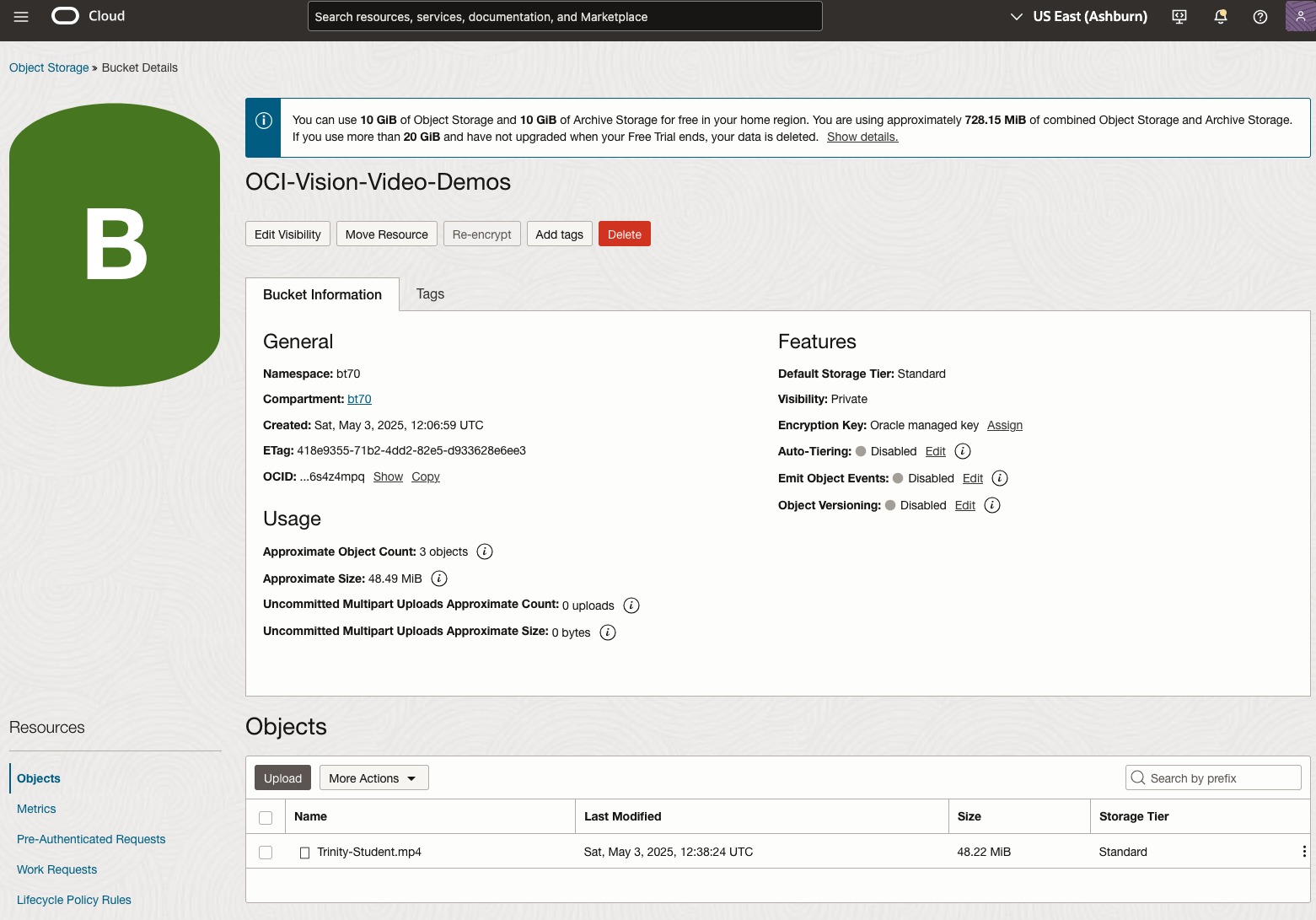
You might need to allow Pre-Authenticated Requests for this bucket. If you don’t do this, you will be prompted by the tool to allow this.
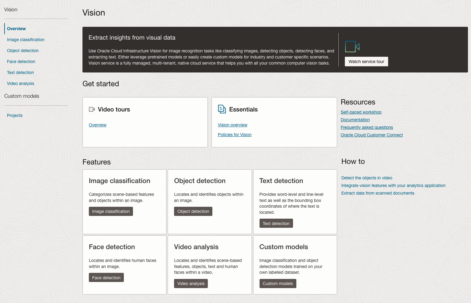
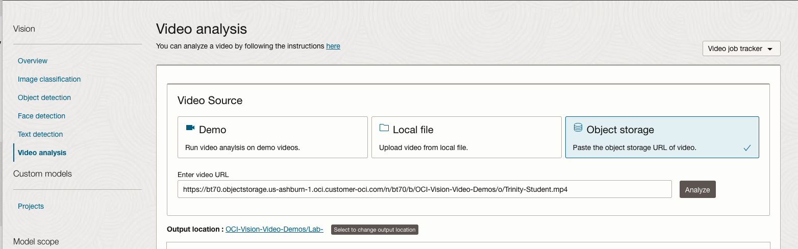
Next, go to the OCI Vision page. You’ll find the Video Analysis tool at the bottom of the menu on the left-hand side of the page.
You can check out the demo videos, or load your own video from the Local File system of you computer, or use a file from your OCI Storage. If you select a video from the Local File system, the video will be loaded in the object storage before it is processed.
For this example, I’m going to use the video I uploaded earlier called Trinity-Student.mp4. Copy the link to this file from the file information in object storage.
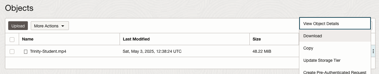
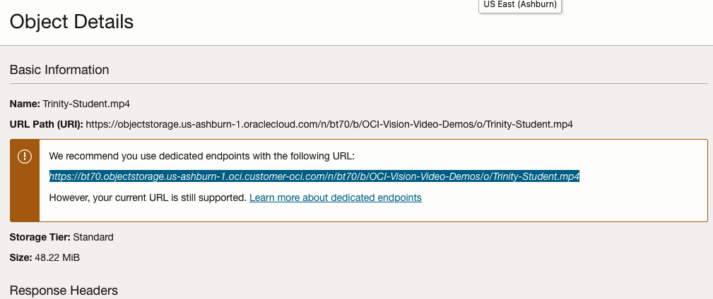
On the Video Analysis page, select Object Storage and paste the link to the file into the URL field. Then click Analyze button. It is at this point that you might get asked to Generate a PAR URL. Do this and then proceed.
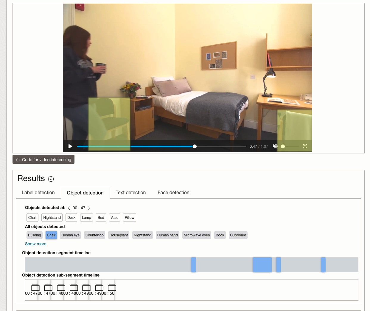
While the video is being parsed, it will appear on the webpage and will start playing. When the video has been Analyzed the details will be displayed below the video. The Analysis will consist of Label Detection, Object Detection, Text Dection and Face Detection.
By clicking on each of these, you’ll see what has been detected, and by clicking on each of these, you’ll be able to see where in the video they were detected. For example, where a Chair was detected.
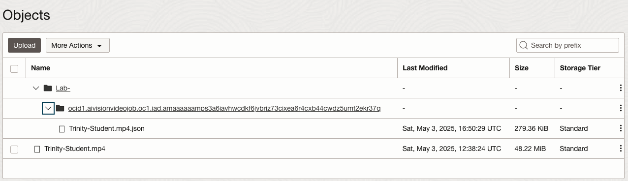
You can also inspect the JSON file containing all the details of various objects detected in the video and the location in the videos they can be found.
This JSON response file is also saved to Object Storage in the same directory, or a sub-directory, where the video is located.
OCI Text to Speech example
In this post, I’ll walk through the steps to get a very simple example of Text-to-Speech working. This example builds upon my previous posts on OCI Language, OCI Speech and others, so make sure you check out those posts.
The first thing you need to be aware of, and to check, before you proceed, is whether the Text-to-Speech is available in your region. At the time of writing, this feature was only available in Phoenix, which is one of the cloud regions I have access to. There are plans to roll it out to other regions, but I’m not aware of the timeline for this. Although you might see Speech listed on your AI menu in OCI, that does not guarantee the Text-to-Speech feature is available. What it does mean is the text trans scribing feature is available.
So if Text-to-Speech is available in your region, the following will get you up and running.
The first thing you need to do is read in the Config file from the OS.
#initial setup, read Config file, create OCI Client
import oci
from oci.config import from_file
##########
from oci_ai_speech_realtime import RealtimeSpeechClient, RealtimeSpeechClientListener
from oci.ai_speech.models import RealtimeParameters
##########

CONFIG_PROFILE = "DEFAULT"
config = oci.config.from_file('~/.oci/config', profile_name=CONFIG_PROFILE)
###
ai_speech_client = ai_speech_client = oci.ai_speech.AIServiceSpeechClient(config)
###
print(config)
### Update region to point to Phoenix
config.update({'region':'us-phoenix-1'})
A simple little test to see if the Text-to-Speech feature is enabled for your region is to display the available list of voices.
list_voices_response = ai_speech_client.list_voices(
    compartment_id=COMPARTMENT_ID,
    display_name="Text-to-Speech")
#    opc_request_id="1GD0CV5QIIS1RFPFIOLF<unique_ID>")

# Get the data from response
print(list_voices_response.data)
This produces a long json object with many characteristics of the available voices. A simpler listing gives the names and gender)
for i in range(len(list_voices_response.data.items)):
    print(list_voices_response.data.items[i].display_name + ' [' + list_voices_response.data.items[i].gender + ']\t' + list_voices_response.data.items[i].language_description )
------
Brian [MALE]	English (United States)
Annabelle [FEMALE]	English (United States)
Bob [MALE]	English (United States)
Stacy [FEMALE]	English (United States)
Phil [MALE]	English (United States)
Cindy [FEMALE]	English (United States)
Brad [MALE]	English (United States)
Richard [MALE]	English (United States)
Now lets setup a Text-to-Speech example using the simple text, Hello. My name is Brendan and this is an example of using Oracle OCI Speech service. First lets define a function to save the audio to a file.
def save_audi_response(data):
    with open(filename, 'wb') as f:
        for b in data.iter_content():
            f.write(b)
    f.close()
We can now establish a connection, define the text, call the OCI Speech function to create the audio, and then to save the audio file.
import IPython.display as ipd

# Initialize service client with default config file
ai_speech_client = oci.ai_speech.AIServiceSpeechClient(config)

TEXT_DEMO = "Hello. My name is Brendan and this is an example of using Oracle OCI Speech service"

#speech_response = ai_speech_client.synthesize_speech(compartment_id=COMPARTMENT_ID)

speech_response = ai_speech_client.synthesize_speech(
    synthesize_speech_details=oci.ai_speech.models.SynthesizeSpeechDetails(
        text=TEXT_DEMO,
        is_stream_enabled=True,
        compartment_id=COMPARTMENT_ID,

        configuration=oci.ai_speech.models.TtsOracleConfiguration(
            model_family="ORACLE",
            model_details=oci.ai_speech.models.TtsOracleTts2NaturalModelDetails(
                model_name="TTS_2_NATURAL",
                voice_id="Annabelle"),
            speech_settings=oci.ai_speech.models.TtsOracleSpeechSettings(
                text_type="SSML",
                sample_rate_in_hz=18288,
                output_format="MP3",
                speech_mark_types=["WORD"])),

        audio_config=oci.ai_speech.models.TtsBaseAudioConfig(config_type="BASE_AUDIO_CONFIG") #, save_path='I'm not sure what this should be')
    ) )

# Get the data from response
#print(speech_response.data)
save_audi_response(speech_response.data)
You must be logged in to post a comment.