
Working with Vector Data and Oracle SQL Command Line SQLcl
Working with Vector data has been a hot topic over the past couple of years. There are lots and articles and blog posts showing some basic functionality and similarity search using Vectors. Most of these articles demonstrate the basics, but then you start working with Vector data and perhaps having to move this data between schemas or between databases you could face a little bit of a challenge. One of these challenges or perhaps compatibility issues is with the format of the Vector data in the output/input file. In the example below I’m going to use CSV file to illustrate the issue, and specifically with using Oracle SQLcl and the export/import to/from CSV file feature.
It should be noted that the issued described below might not be an issue in a future release of SQLcl. I’ve reported this issue and a bug report has been filled. So fingers cross it will be fixed soon and even back ported. So the workaround or fix illustrated below might not be necessary at some point in the future, but until such time the workaround below is required.
The basic secenario that I faced involved exporting a table, containing Vector data, and importing it into a different (empty) table in the same schema. The export feature seemed to work correctly but I get an error when importing the file. Something about the work data type etc. It was complaining about the Vector column format. After a little investigation, the export command exported the data but the Vector column did not have quotes around the data. The import command expected the Vector data to be in quotes. So there is a mismatch between the export and import commands for Vector data.

Here is a bit more detail on how I encountered this issue.
I created a table to store Wine Reviews, Imported the Wine Review data set. added a column to store the Vector Data, added the Vector data using a model I’d already imported. I then exported the Wine Reviews with the Vector data to CSV. I unloaded the table using the following SQL Command Line function UNLOAD
sql> unload wine_reviews
This created a file in my working directory called WINEREVIEWS_TABLE.csv
I then created a new version of the table with a different name, WINEREVIEWS_VEC, and used the LOAD function to load the CSV data into the the newly created table.
sql> load WINEREVIEWS_VEC WINEREVIEWS_TABLE.csv
This gives me the following error.
#ERROR Insert failed in batch rows 1 through 50#ERROR ORA-51804: Invalid syntax for VECTOR value. Must be a string of the formDENSE vector: '[<number> , <number> ..., <number>]'SPARSE vector: '[<total dimension count (optional)>, [<sparse index array>], [<sparse dimension value array>]]'.
What this error means is the Vector data is missing a quote at the beginning and end of the vector data.
So what can we do to fix this issue and move forward with import and being able to use the data.
In my case I used the ‘sed’ command, and here is the one line ‘sed’ command to add the quotes around the required field.
sed 's/,\(\[[^]]*\]\)/,"\1"/g' WINEREVIEWS_TABLE.csv > WINEREVIEWS_TABLE_vec.csv

No using he same LOAD function as previously used, the import/load works and is completed in a couple of seconds.
Before we end this post, lets have another look at the ‘sed’ command and what it does, as you can see it is a little complicated.
sed 's/,\(\[[^]]*\]\)/,"\1"/g' WINEREVIEWS_TABLE.csv > WINEREVIEWS_TABLE_vec.csv
The main focus of this command is to look for fields that are enclosed by square brackets [ ]. When you look at the CSV file, only the vector data is enclose in such brackets. what we need to do is to wrap this in quotes, as otherwise the comma in these brackets will be considered as field/column separators.
Breaking down the pattern ,\(\[[^]]*\]\)

So the whole thing matches: a comma, immediately followed by a bracketed block like [anything except ]], and captures that bracketed block (brackets included) as group 1.
The replacement ,"\1" puts back the comma, then wraps the captured bracket block in double quotes.
The g flag makes it do this for every match on the line, not just the first.
6 Things the Council Just Changed in the EU AI Act
The Council of the EU just signed off on the amendments to the AI Act and yes, the high-risk deadlines are moving. Let’s have a look at what’s actually in there, because there’s more going on than just a delay.
Timing first, since that’s what everyone’s asking about:
- Annex III high-risk systems: pushed to 2 December 2027
- Annex I high-risk systems: pushed to 2 August 2028
- National AI regulatory sandboxes: authorities now have until 2 August 2027 to get these running
- Transparency obligations for AI-generated content: grace period runs out 2 December 2026
A new practice gets added to the banned list. Generating non-consensual sexual or intimate content, or CSAM, is now explicitly prohibited. That covers tools that produce nude images of real people or strip clothing out of existing photos. This one bites from December 2026.
The AI Office’s job just got clearer. Where a provider builds both the general-purpose model and the system on top of it, the AI Office is the one supervising. National authorities still keep their patch though — think law enforcement, border control, courts, and financial services.
Sectoral law and the AI Act don’t have to fight each other anymore. If you’re building something in Annex I that’s already covered by product-specific rules (medical devices, lifts, toys, watercraft, that kind of thing), and those rules already demand AI-specific safeguards similar to the Act’s, the AI Act steps back rather than piling on.
Machinery gets a carve-out. Products under the machinery regulation that used to sit in Annex I as high-risk are no longer directly caught by the AI Act. Instead, the Commission can add health and safety requirements through machinery-specific secondary legislation.
And the Commission has to actually help you comply. For Annex I providers already juggling sectoral law, the Commission is now on the hook to produce guidance that keeps the compliance burden as light as possible.
Net effect: more breathing room on timing, but also a genuine attempt to stop the AI Act and existing product law from overlapping and creating double work. Worth building into your compliance roadmap now rather than waiting for the deadlines to get closer.
Oracle Semantic Search using Vectors on Iceberg Tables
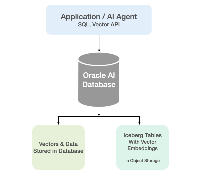
In my previous blog posts I’ve explored how to use Iceberg Tables and how to integrate these in with your Data Lake. Additionally, I showed how to setup your Oracle Data Lake (Database) to access the data stored in Iceberg Tables stored in OCI Object Storage. To access this Iceberg Table data from the Oracle Database we created an External Table. This allows us to query the Iceberg Table data as if it was internal to the database. With all new releases there is continuous improvement in the features and to make them easier to use. One such new feature (as of 23.26.1) is the ability to read vector data types from an External Table. This new feature is called or referred to as ‘Vectors on Ice’.
With Oracle Database External Tables now supporting vector embedding stored in Iceberg Tables, means you can generate vector embeddings with your preferred embedding model (external to Oracle using your faviourite tool/library), store them in Iceberg Tables in cloud object storage (OCI Object Storage, AWS S3, etc.), and run semantic search from Oracle AI Database, accessing vector data stored within the database and externally with the minimum of data movement and with similar SQL queries.
Summary: Vectors on Ice lets you ask semantic questions of your data lake using the same SQL and vector search tooling you already use in Oracle Database, without copying or moving the data.
Oracle vector indexes can be created to speed up semantic search over the vectors in the Iceberg Tables. You don’t need to copy Iceberg data into an Oracle Database to use them or to update the Vector Index. The vector indexes are stored standalone in the database and (depending on the type of Vector Index used) can automatic sync as data is added to the files on Object Storage. The syncing of the Vector Index is not immediately updated but is updated based on a background process, so you can look on this index being eventually consistent. In might happen fairly quickly or during large write periods in might take seconds to a few minutes to get fully up-to-date.
Let’s have a look at an example of this. The following example builds upon my example in my previous posts which walked through the setup sets needed for gaining access to Object Storage, etc
CREATE TABLE IF NOT EXISTS external_vector_file ( id VARCHAR(10) PRIMARY KEY, text_desc VARCHAR2(1000), vec_embedding VECTOR(1024, float32) ) ORGANIZATION EXTERNAL ( TYPE ORACLE_BIGDATA DEFAULT DIRECTORY DATA_PUMP_DIR ACCESS PARAMETERS ( com.oracle.bigdata.credential.name=OCI_CRED com.oracle.bigdata.fileformat=parquet com.oracle.bigdata.access_protocol=iceberg ) LOCATION ('<path-to-iceberg-table>/metadata/v1.metadata.json') ) REJECT LIMIT UNLIMITED;
and to create a Vector Index on this external file
CREATE VECTOR INDEX external_vector_file_idx_ivf ON external_vector_file (vec_embedding)ORGANIZATION NEIGHBOR PARTITIONS;
We can now run our SQL queries on this external vector data. This query assumes we have the same vector embedding model loaded into the database.
SELECT id, text_desc, vector_distance(vec_embedding, vector_embedding(my_onnx_model using :INPUT_TERM as data) DISTFROM external_vector_fileORDER BY DISTFETCH FIRST 10 ROWS ONLY;
Why is this important? This allows organisations that already store vectors or embeddings in Iceberg Tables, as part of an existing ML pipeline, and who want to query them, performing semantic search, alongside the data in their Oracle Database, can now do so with the minimum of setup. This brings the benefits of Semantic Search to a wider audience within the organisation.
Exploring Apache Iceberg – Part 5 – Iceberg Tables and Oracle Autonomous Database
I’ve been writing a series of posts on using Apache Iceberg tables, and this fifth post will focus on using the Iceberg Tables in the Oracle LakeHouse Databae or Oracle Autonomous Data Warehouse database. Make sure to check out the previous posts as some of the steps needed to create the Iceberg files and some initital setup in an Oracle Autonomous Database. Here’s the link to Part-4.
For the example below I’ve already pre-loaded the Iceberg Table catalog and associated set of files. For this I’ve uploaded the files into a bucket called ‘iceberg-lakehouse’ and you’ll see references to this in the examples below.
One of the first things you’ll need to to is to grant certain privileges to your schema to allow it to use the Lakehouse features, like working with Iceberg Tables, setting up the Access Control Lists if needed and to have access to the DBMS_CATALOG package.
Here is the url for the ‘iceberg-lakehouse’. I’ve removed my nampespace from the url. When you setup your own one the part with <namespace> will contain the name of for your tenency.
https://objectstorage.us-ashburn-1.oraclecloud.com/n/<namespace>/b/iceberg-lakehouse/o/
The schema I’m using the the database is called ‘brendan’. Yes I could have been more creative!
Grant the DWROLE to the schema that will contain the external table to the Iceberg Table. Do this using ADMIN. Permissions on DBMS_CLOUD is also needed.
grant DWROLE to brendan;grant execute on DBMS_CLOUD to brendan;
While still connected to ADMIN, we need to configure an Access Control List (ACL) for the Lakehouse schema.
BEGIN DBMS_NETWORK_ACL_ADMIN.APPEND_HOST_ACE( host => 'objectstorage.us-ashburn-1.oraclecloud.com', lower_port => 443, upper_port => 443, ace => xs$ace_type( privilege_list => xs$name_list('http'), principal_name => 'BRENDAN', -- the Lakehouse schema principal_type => xs_acl.ptype_db ) );END;
My tenency is based in Ashburn, and that’s why you see ‘us-ashburn-1’ listed in the value for host, given in the above example. You’ll need to change that to your region.
As the ‘BRENDAN’ schema we can define Credentials to autenticate to OCI Object Storage.
BEGIN DBMS_CLOUD.CREATE_CREDENTIAL( credential_name => 'LAKEHOUSE_CRED', username => '<your cloud username>', password => '<generated auth token>' );END;
Now we can create an External Table to point to our Iceberg Table.
BEGIN DBMS_CLOUD.CREATE_EXTERNAL_TABLE( table_name => 'ICEBERG_TABLE', credential_name => 'LAKEHOUSE_CRED', file_uri_list => 'https://objectstorage.us-ashburn-1.oraclecloud.com/n/<namespace>/b/iceberg-lakehouse/o/', format => '{"access_protocol": {"protocol_type": "iceberg"}}' );END;
We can not query the Iceberg Table like a regular table.
select * from iceberg_table;
Important: When work with the scenario above, it is assumed the Iceberg Table contains only one table. Another limitation is, if the structure of the Iceberg Table changes you will need to re-create the external table. As you can imagine that is not ideal, although you can schedule that to happen as needed.
To over come those limitations and to allow for the Iceberg Catalog to contain multiple tables, and for those to be picked up automatically, we need to use the package DBMS_CATALOG. This allows use to work with multiple tables within the catalog and it will also pickup any schema changes to those Iceberg Tables. Let’s have a look at doing this.
There are two steps needed before creating the external table. Both create credentials to point to the external Iceberg REST catalog and another to point to the bucket in object storage where the data files are located.
-- create credential for the REST API link to the catalogBEGIN DBMS_CLOUD.CREATE_CREDENTIAL( credential_name => 'ICEBERG_CATALOG_CRED', username => '<username for REST API>', password => '<password for REST API>' );END;
The REST API details can be found in your OCI accout under Users & Security-> Users.
The OCI Object Storage Credentials is where the data files are stored in an OCI bucket. We can now mount the Iceberg Catalog
BEGIN DBMS_CATALOG.MOUNT_ICEBERG( catalog_name => 'ICEBEG_CATALOG', endpoint => '<endpoint for the catalog>', catalog_credential => 'ICEBERG_CATALOG_CRED', data_storage_credential => '<OCI Object Storge Credential>' );END;
Once mounted we can explore the tables available in the Catalog using,
select * from all_tables@ICEBERG_CATALOG;
When querying the tables in the catalog, it will resolve to the latest snapshot. [see previous posts on how the catalog and the following tabl was created]
select * from sales_db.orders@ICEBERG_CATALOG;
If we want the Iceberg table to be used as an External Table in the database we can create it using the following.
BEGIN DBMS_CATALOG.CREATE_EXTERNAL_TABLE( catalog_name => 'ICEBERG_CATALOG', table_name => 'ICEBERG_ORDERS', schema_name => 'sales_db', table_name => 'orders' );END;
It is now a bit easier to include in our queries.
select * from ICEBERG_ORDERS;
Exploring Apache Iceberg – Part 4 – Parquet Files with Oracle Autonomous Database
In this post I’ll walk through the steps needed to setup and use Parquet files with an Oracle Autonomous Database and with the parquet files stored in Oracle Cloud. In my previous post, did something similar but for an on-premises Oracle Database.
Generally the setup is very similar except for two particular parts where we need to load the parquet files into a bucket on Oracle cloud (OCI) and the secondly we need some additional configuration in the Database to be able to access those files in an OCI bucket.
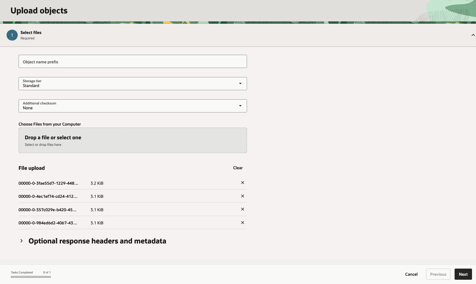
Create Bucket and Upload files
In OCI Storage section of OCI, create a new bucket (Parquet-files) and upload the parquet files. You can automate this step with a simple piece of Python code.
Create Credential
Log into the schema you are going to use to create the external table. You’ll need to generate an authentication token.
BEGIN DBMS_CLOUD.CREATE_CREDENTIAL( credential_name => 'PARQUET_FILES_CRED', username => '<your cloud username>', password => '<generated auth token>' );END;
Create the External table
We can now create the external table pointing to the parquet files in the OCI bucket.
BEGIN DBMS_CLOUD.CREATE_EXTERNAL_TABLE( table_name => 'PARQUET_FILES_EXT', credential_name => 'PARQUET_FILES_CRED', file_uri_list => 'https://objectstorage.us-ashburn-1.oraclecloud.com/n/<namespace>/b/Parquet-Files/o/*.parquet', format => JSON_OBJECT( 'type' VALUE 'parquet', 'schema' VALUE 'first', 'blankasnull' VALUE 'true', 'trimspaces' VALUE 'lrtrim' ) );END;/
Query the Parquet Files
We can now query the parquet files.
SELECT region, product, SUM(amount) AS total_salesFROM parquet_files_extGROUP BY regionORDER BY total_sales DESC;
Exploring Apache Iceberg – Part 3 – Parquet Files with Oracle Database
In this post I’ll explore how you can included data in Parquet files in an Oracle Database. This is a little sideways post from my previous posts on Apache Iceberg, as it will only look at using Parquet files, which are a core part of Iceberg tables, but is missing the meta-data layer that Iceberg tables gives.
The previous two posts on Apache Iceberg looked at using PyIceberg Python package to create and to explore the various feature of Iceberg and it’s effects on the data, files and meta-data. Part-1, Part-2.
We can include Parquet files in an Oracle Database by creating an External Table based on those files. Let’s walk through an example. The following example will for an “On-Premises” Database. I’ll have an example later in this post if you are using an Oracle Autonomous Database on Oracle Cloud.
Log into the Database as SYSTEM user, create a directory option to point to the location of the files on the operating system, and then grant privileges to the schama that needs to read that data.
CREATE OR REPLACE DIRECTORY parquet_dir AS '/data/log/parquet';GRANT READ, WRITE ON DIRECTORY parquet_dir TO parquet_user;
It is assumed the directory ‘/data/log/parquet‘ exists and has some parquet files in it.
Connect the schama “parquet_user” and create an External Table that points to the parquet files in the directory
CREATE TABLE parquet_sales_data ( sale_id NUMBER, sale_date DATE, product_id NUMBER, amount NUMBER(10,2), region VARCHAR2(50))ORGANIZATION EXTERNAL ( TYPE ORACLE_BIGDATA DEFAULT DIRECTORY parquet_dir ACCESS PARAMETERS ( com.oracle.bigdata.fileformat = PARQUET ) LOCATION ('sales_*.parquet'))REJECT LIMIT UNLIMITED;
We can not query the parquey data just like any other data in a table.
SELECT region, product, SUM(amount) AS total_salesFROM sales_externalGROUP BY regionORDER BY total_sales DESC;
Care is needed to ensure column name and datatypes match between the table and the parquet file.
If our parquet files are partitioned into directories for different time periods, we can create a Partitioned External Table to handle that data, and we it we get the benefits of partition pruning, etc and better response times.
CREATE TABLE parquet_sales_data ( sale_id NUMBER, sale_date DATE, product_id NUMBER, amount NUMBER(10,2), region VARCHAR2(50))ORGANIZATION EXTERNAL PARALLEL 4 ( TYPE ORACLE_BIGDATA DEFAULT DIRECTORY parquet_dir ACCESS PARAMETERS ( com.oracle.bigdata.fileformat = PARQUET )PARTITION BY LIST (region) ( PARTITION p_emea VALUES ('EMEA') LOCATION (emea_dir:'*.parquet'), PARTITION p_apac VALUES ('APAC') LOCATION (apac_dir:''*.parquet'), PARTITION p_amer VALUES ('AMER') LOCATION (amer_dir:'*.parquet'))REJECT LIMIT UNLIMITED;
For this example, I needed to connect as SYSTEM and create the extra directories to point to the additional directories used. I also added PARALLEL 4 to the table to help speed things up a little more.
Exploring Apache Iceberg using PyIceberg – Part 2
Apache Iceberg, an open-source table format that has become the industry standard for data sharing in modern data architectures. In my previous posts on Apache Iceberg I explored the core features of Iceberg Tables and gave examples of using Python code to create, store, add data, read a table and apply filters to an Iceberg Table. In this post I’ll explore some of the more advanced features of interacting with an Iceberg Table, how to add partitioning and how to moved data to a DuckDB database.
Check out the link at the bottom of this post to download the Notebook containing all the PyIceberg code in this post. I had a similar notebook for all the code examples in my previous post. You should check that our first as the examples in the post and notebook are an extension of those.
This post will cover:
- Partitioning an Iceberg Table
- Schema Evolution
- Row Level Operations
- Advanced Scanning & Query Patterns
- DuckDB and Iceberg Tables
Setup & Conguaration
Before we can start on the core aspects of this post, we need to do some basic setup like importing the necessary Python packages, defining the location of the warehouse and catalog and checking the namespace exists. These were created created in the previous post.
import os, pandas as pd, pyarrow as pafrom datetime import datefrom pyiceberg.catalog.sql import SqlCatalogfrom pyiceberg.schema import Schemafrom pyiceberg.types import ( NestedField, LongType, StringType, DoubleType, DateType)from pyiceberg.partitioning import PartitionSpec, PartitionFieldfrom pyiceberg.transforms import ( MonthTransform, IdentityTransform, BucketTransform)WAREHOUSE = "/Users/brendan.tierney/Dropbox/Iceberg-Demo"os.makedirs(WAREHOUSE, exist_ok=True)catalog = SqlCatalog("local", **{ "uri": f"sqlite:///{WAREHOUSE}/catalog.db", "warehouse": f"file://{WAREHOUSE}",})for ns in ["sales_db"]: if ns not in [n[0] for n in catalog.list_namespaces()]: catalog.create_namespace(ns)
Partitioning an Iceberg Table
Partitioning is how Iceberg physically organises data files on disk to enable partition pruning. Partitioning pruning will automactically skip directorys and files that don’t contain the data you are searching for. This can have a significant improvement of query response times.
The following will create a partition table based on the combination of the fiels order_date and region.
# ── Explicit Iceberg schema (gives us full control over field IDs) ─────schema = Schema( NestedField(field_id=1, name="order_id", field_type=LongType(), required=False), NestedField(field_id=2, name="customer", field_type=StringType(), required=False), NestedField(field_id=3, name="product", field_type=StringType(), required=False), NestedField(field_id=4, name="region", field_type=StringType(), required=False), NestedField(field_id=5, name="order_date", field_type=DateType(), required=False), NestedField(field_id=6, name="revenue", field_type=DoubleType(), required=False),)# ── Partition spec: partition by month(order_date) AND identity(region) ─partition_spec = PartitionSpec( PartitionField( source_id=5, # order_date field_id field_id=1000, transform=MonthTransform(), name="order_date_month", ), PartitionField( source_id=4, # region field_id field_id=1001, transform=IdentityTransform(), name="region", ),)tname = ("sales_db", "orders_partitioned")if catalog.table_exists(tname): catalog.drop_table(tname)
Now we can create the table and inspect the details
table = catalog.create_table( tname, schema=schema, partition_spec=partition_spec,)print("Partition spec:", table.spec())Partition spec: [ 1000: order_date_month: month(5) 1001: region: identity(4)]
We can now add data to the partitioned table.
# Write data — Iceberg routes each row to the correct partition directorydf = pd.DataFrame({ "order_id": [1001, 1002, 1003, 1004, 1005, 1006], "customer": ["Alice", "Bob", "Carol", "Dave", "Eve", "Frank"], "product": ["Laptop", "Phone", "Tablet", "Monitor", "Keyboard", "Webcam"], "region": ["EU", "US", "EU", "APAC", "US", "EU"], "order_date": [date(2024,1,15), date(2024,1,20), date(2024,2,3), date(2024,2,20), date(2024,3,5), date(2024,3,12)], "revenue": [1299.99, 1798.00, 549.50, 1197.00, 399.95, 258.00],})table.append(pa.Table.from_pandas(df))
We can inspect the directories and files created. I’ve only include a partical listing below but it should be enough for you to get and idea of what Iceberg as done.
# Verify partition directories were created!find {WAREHOUSE}/sales_db/orders_partitioned/data -type f/Users/brendan.tierney/Dropbox/Iceberg-Demo/sales_db/orders_partitioned/data/region=APAC/order_date_day=2024-04-05/00000-4-0542db6c-f67f-4a26-9012-59d8267b5005.parquet/Users/brendan.tierney/Dropbox/Iceberg-Demo/sales_db/orders_partitioned/data/region=APAC/order_date_day=2024-02-20/00000-2-0542db6c-f67f-4a26-9012-59d8267b5005.parquet/Users/brendan.tierney/Dropbox/Iceberg-Demo/sales_db/orders_partitioned/data/order_date_month=2024-01/region=EU/00000-0-e9ad65a0-c088-46fc-a537-12a6b60b38c5.parquet/Users/brendan.tierney/Dropbox/Iceberg-Demo/sales_db/orders_partitioned/data/order_date_month=2024-01/region=EU/00000-0-1f976101-f836-4db3-bf4a-c0e0cf7dd4c6.parquet/Users/brendan.tierney/Dropbox/Iceberg-Demo/sales_db/orders_partitioned/data/order_date_month=2024-01/region=EU/00000-0-4233dad6-ef48-4ad5-95c9-5842e641fc0f.parquet/Users/brendan.tierney/Dropbox/Iceberg-Demo/sales_db/orders_partitioned/data/order_date_month=2024-01/region=EU/00000-0-b0a10298-d2a6-45b4-a541-9a459e478496.parquet/Users/brendan.tierney/Dropbox/Iceberg-Demo/sales_db/orders_partitioned/data/order_date_month=2024-01/region=US/00000-1-b0a10298-d2a6-45b4-a541-9a459e478496.parquet/Users/brendan.tierney/Dropbox/Iceberg-Demo/sales_db/orders_partitioned/data/order_date_month=2024-01/region=US/00000-1-4233dad6-ef48-4ad5-95c9-5842e641fc0f.parquet/Users/brendan.tierney/Dropbox/Iceberg-Demo/sales_db/orders_partitioned/data/order_date_month=2024-01/region=US/00000-1-1f976101-f836-4db3-bf4a-c0e0cf7dd4c6.parquet/Users/brendan.tierney/Dropbox/Iceberg-Demo/sales_db/orders_partitioned/data/order_date_month=2024-01/region=US/00000-1-e9ad65a0-c088-46fc-a537-12a6b60b38c5.parquet/Users/brendan.tierney/Dropbox/Iceberg-Demo/sales_db/orders_partitioned/data/region=EU/order_date_day=2024-02-03/00000-1-0542db6c-f67f-4a26-9012-59d8267b5005.parquet/Users/brendan.tierney/Dropbox/Iceberg-Demo/sales_db/orders_partitioned/data/region=EU/order_date_day=2024-01-15/00000-0-0542db6c-f67f-4a26-9012-59d8267b5005.parquet/Users/brendan.tierney/Dropbox/Iceberg-Demo/sales_db/orders_partitioned/data/region=EU/order_date_day=2024-04-01/00000-3-0542db6c-f67f-4a26-9012-59d8267b5005.parquet/Users/brendan.tierney/Dropbox/Iceberg-Demo/sales_db/orders_partitioned/data/order_date_month=2024-02/region=APAC/00000-3-b0a10298-d2a6-45b4-a541-9a459e478496.parquet/Users/brendan.tierney/Dropbox/Iceberg-Demo/sales_db/orders_partitioned/data/order_date_month=2024-02/region=APAC/00000-3-e9ad65a0-c088-46fc-a537-12a6b60b38c5.parquet/Users/brendan.tierney/Dropbox/Iceberg-Demo/sales_db/orders_partitioned/data/order_date_month=2024-02/region=APAC/00000-3-4233dad6-ef48-4ad5-95c9-5842e641fc0f.parquet/Users/brendan.tierney/Dropbox/Iceberg-Demo/sales_db/orders_partitioned/data/order_date_month=2024-02/region=APAC/00000-3-1f976101-f836-4db3-bf4a-c0e0cf7dd4c6.parquet
We can change the partictioning specification without rearranging or reorganising the data
from pyiceberg.transforms import DayTransform# Iceberg can change the partition spec without rewriting old data.# Old files keep their original partitioning; new files use the new spec.with table.update_spec() as update: # Upgrade month → day granularity for more recent data update.remove_field("order_date_month") update.add_field( source_column_name="order_date", transform=DayTransform(), partition_field_name="order_date_day", )print("Updated spec:", table.spec())
I’ll leave you to explore the additional directories, files and meta-data files.
#find all files starting from this directory!find {WAREHOUSE}/sales_db/orders_partitioned/data -type f
Schema Evolution
Iceberg tracks every schema version with a numeric ID and never silently breaks existing readers. You can add, rename, and drop columns, change types (safely), and reorder fields, all with zero data rewriting.
#Add new columnsfrom pyiceberg.types import FloatType, BooleanType, TimestampTypeprint("Before:", table.schema())with table.update_schema() as upd: # Add optional columns — old files return NULL for these upd.add_column("discount_pct", FloatType(), "Discount percentage applied") upd.add_column("is_returned", BooleanType(), "True if the order was returned") upd.add_column("updated_at", TimestampType())print("After:", table.schema())Before: table { 1: order_id: optional long 2: customer: optional string 3: product: optional string 4: region: optional string 5: order_date: optional date 6: revenue: optional double}After: table { 1: order_id: optional long 2: customer: optional string 3: product: optional string 4: region: optional string 5: order_date: optional date 6: revenue: optional double 7: discount_pct: optional float (Discount percentage applied) 8: is_returned: optional boolean (True if the order was returned) 9: updated_at: optional timestamp}
We can rename columns. A column rename is a meta-data only change. The Parquet files are untouched. Older readers will still see the previous versions of the column name, whicl new readers will see the new column name.
#rename a columnwith table.update_schema() as upd: upd.rename_column("discount_pct", "discount_percent")print("Updated:", table.schema())Updated: table { 1: order_id: optional long 2: customer: optional string 3: product: optional string 4: region: optional string 5: order_date: optional date 6: revenue: optional double 7: discount_percent: optional float (Discount percentage applied) 8: is_returned: optional boolean (True if the order was returned) 9: updated_at: optional timestamp}
Similarly when dropping a column, it is a meta-data change
#drop a columnwith table.update_schema() as upd: upd.delete_column("updated_at")print("Updated:", table.schema())Updated: table { 1: order_id: optional long 2: customer: optional string 3: product: optional string 4: region: optional string 5: order_date: optional date 6: revenue: optional double 7: discount_percent: optional float (Discount percentage applied) 8: is_returned: optional boolean (True if the order was returned)}
We can see all the different changes or versions of the Iceberg Table schema.
import json, globmeta_files = sorted(glob.glob( f"{WAREHOUSE}/sales_db/orders_partitioned/metadata/*.metadata.json"))with open(meta_files[-1]) as f: meta = json.load(f)print(f"Total schema versions: {len(meta['schemas'])}")for s in meta["schemas"]: print(f" schema-id={s['schema-id']} fields={[f['name'] for f in s['fields']]}")Total schema versions: 4 schema-id=0 fields=['order_id', 'customer', 'product', 'region', 'order_date', 'revenue'] schema-id=1 fields=['order_id', 'customer', 'product', 'region', 'order_date', 'revenue', 'discount_pct', 'is_returned', 'updated_at'] schema-id=2 fields=['order_id', 'customer', 'product', 'region', 'order_date', 'revenue', 'discount_percent', 'is_returned', 'updated_at'] schema-id=3 fields=['order_id', 'customer', 'product', 'region', 'order_date', 'revenue', 'discount_percent', 'is_returned']
Agian if you inspect the directories and files in the warehouse, you’ll see the impact of these changes at the file system level.
#find all files starting from this directory!find {WAREHOUSE}/sales_db/orders_partitioned/data -type f
Row Level Operations
Iceberg v2 introduces two delete file formats that enable row-level mutations without rewriting entire data files immediately — writes stay fast, and reads merge deletes on the fly.
Operations Iceberg Mechanism Write cost Read cost Append New data files only Low Low Delete rows Position or equality delete files Low Medium Update rows Delete + new data file Medium Medium (copy-on-write or merge-on-read) Overwrite Atomic swap of data files Medium Low (replace partition).
from pyiceberg.expressions import EqualTo, In# Delete all orders from the APAC regiontable.delete(EqualTo("region", "APAC"))print(table.scan().to_pandas()) order_id customer product region order_date revenue discount_percent \0 1001 Alice Laptop EU 2024-01-15 1299.99 NaN 1 1002 Bob Phone US 2024-01-20 1798.00 NaN 2 1003 Carol Tablet EU 2024-02-03 549.50 NaN 3 1005 Eve Keyboard US 2024-03-05 399.95 NaN 4 1006 Frank Webcam EU 2024-03-12 258.00 NaN is_returned 0 None 1 None 2 None 3 None 4 None
Also
# Delete specific order IDstable.delete(In("order_id", [1001, 1003]))# Verify — deleted rows are gone from the logical viewdf_after = table.scan().to_pandas()print(f"Rows after delete: {len(df_after)}")print(df_after[["order_id", "customer", "region"]])Rows after delete: 3 order_id customer region0 1002 Bob US1 1005 Eve US2 1006 Frank EU
We can see partiton pruning in action with a scan EqualTo(“region”, “EU”) will skip all data files in region=US/ and region=APAC/ directories entirely — zero bytes read from those files.
Advanced Scanning & Query Processing
The full expression API (And, Or, Not, In, NotIn, StartsWith, IsNull), time travel by snapshot ID, incremental reads between two snapshots for CDC pipelines, and streaming via Arrow RecordBatchReader for out-of-memory processing.
PyIceberg’s scan API supports rich predicate pushdown, snapshot-based time travel, incremental reads between snapshots, and streaming via Arrow record batches.
Let’s start by adding some data back into the table.
df3 = pd.DataFrame({ "order_id": [1001, 1003, 1004, 1006, 1007], "customer": ["Alice", "Carol", "Dave", "Frank", "Grace"], "product": ["Laptop", "Tablet", "Monitor", "Headphones", "Webcam"], "order_date": [ date(2024, 1, 15), date(2024, 2, 3), date(2024, 2, 20), date(2024, 4, 1), date(2024, 4, 5)], "region": ["EU", "EU", "APAC", "EU", "APAC"], "revenue": [1299.99, 549.50, 1197, 498.00, 129.00]})#Add the datatable.append(pa.Table.from_pandas(df3))
Let’s try a query with several predicates.
from pyiceberg.expressions import ( And, Or, Not, EqualTo, NotEqualTo, GreaterThan, GreaterThanOrEqual, LessThan, LessThanOrEqual, In, NotIn, IsNull, IsNaN, StartsWith,)# EU or US orders, revenue > 500, product is not "Keyboard"df_complex = table.scan( row_filter=And( Or( EqualTo("region", "EU"), EqualTo("region", "US"), ), GreaterThan("revenue", 500.0), NotEqualTo("product", "Keyboard"), ), selected_fields=("order_id", "customer", "product", "region", "revenue"),).to_pandas()print(df_complex) order_id customer product region revenue0 1001 Alice Laptop EU 1299.991 1003 Carol Tablet EU 549.502 1002 Bob Phone US 1798.00
Now let’s try a NOT predicate
df_not_in = table.scan( row_filter=Not(In("region", ["US", "APAC"]))).to_pandas()print(df_not_in) order_id customer product region order_date revenue \0 1001 Alice Laptop EU 2024-01-15 1299.99 1 1003 Carol Tablet EU 2024-02-03 549.50 2 1006 Frank Headphones EU 2024-04-01 498.00 3 1006 Frank Webcam EU 2024-03-12 258.00 discount_percent is_returned 0 NaN None 1 NaN None 2 NaN None 3 NaN None
Now filter data with data starting with certain values.
df_starts = table.scan( row_filter=StartsWith("product", "Lap") # matches "Laptop", "Laptop Pro").to_pandas()print(df_starts) order_id customer product region order_date revenue discount_percent \0 1001 Alice Laptop EU 2024-01-15 1299.99 NaN is_returned 0 None
Using the LIMIT function.
df_sample = table.scan(limit=3).to_pandas()print(df_sample) order_id customer product region order_date revenue discount_percent \0 1001 Alice Laptop EU 2024-01-15 1299.99 NaN 1 1003 Carol Tablet EU 2024-02-03 549.50 NaN 2 1004 Dave Monitor APAC 2024-02-20 1197.00 NaN is_returned 0 None 1 None 2 None
We can also perform data streaming.
# Process very large tables without loading everything into memory at oncescan = table.scan(selected_fields=("order_id", "revenue"))total_revenue = 0.0total_rows = 0# to_arrow_batch_reader() returns an Arrow RecordBatchReaderfor batch in scan.to_arrow_batch_reader(): df_chunk = batch.to_pandas() total_revenue += df_chunk["revenue"].sum() total_rows += len(df_chunk)print(f"Total rows: {total_rows}")print(f"Total revenue: ${total_revenue:,.2f}")Total rows: 8Total revenue: $6,129.44
DuckDB and Iceberg Tables
We can register an Iceberg scan plan as a DuckDB virtual table. PyIceberg handles metadata; DuckDB reads the Parquet files.
conn = duckdb.connect()# Expose the scan plan as an Arrow dataset DuckDB can queryscan = table.scan()arrow_dataset = scan.to_arrow() # or to_arrow_batch_reader()conn.register("orders", arrow_dataset)# Full SQL on the tableresult = conn.execute(""" SELECT region, COUNT(*) AS order_count, ROUND(SUM(revenue), 2) AS total_revenue, ROUND(AVG(revenue), 2) AS avg_revenue, ROUND(MAX(revenue) - MIN(revenue), 2) AS revenue_range FROM orders GROUP BY region ORDER BY total_revenue DESC""").df()print(result) region order_count total_revenue avg_revenue revenue_range0 EU 4 2605.49 651.37 1041.991 US 2 2197.95 1098.97 1398.052 APAC 2 1326.00 663.00 1068.00
DuckDB has a native Iceberg extension that reads Parquet files directly.
import duckdb, globconn = duckdb.connect()conn.execute("INSTALL iceberg; LOAD iceberg;")# Enable version guessing for Iceberg tablesconn.execute("SET unsafe_enable_version_guessing = true;")# Point DuckDB at the Iceberg table root directorytable_path = f"{WAREHOUSE}/sales_db/orders_partitioned"df_duck = conn.execute(f""" SELECT * FROM iceberg_scan('{table_path}', allow_moved_paths = true) WHERE revenue > 500 ORDER BY revenue DESC""").df()print(df_duck) order_id customer product region order_date revenue discount_percent \0 1002 Bob Phone US 2024-01-20 1798.00 NaN 1 1001 Alice Laptop EU 2024-01-15 1299.99 NaN 2 1004 Dave Monitor APAC 2024-02-20 1197.00 NaN 3 1003 Carol Tablet EU 2024-02-03 549.50 NaN is_returned 0 <NA> 1 <NA> 2 <NA> 3 <NA>
We can access the data using the time travel Iceberg feature.
# Time travel via DuckDBsnap_id = table.history()[0].snapshot_iddf_tt = conn.execute(f""" SELECT * FROM iceberg_scan( '{table_path}', snapshot_from_id = {snap_id}, allow_moved_paths = true )""").df()print(f"Time travel rows: {len(df_tt)}")Time travel rows: 6
How to download a Kaggle Competition dataset
Kaggle is a popular website for data science and machine learning, where users can participate in machine learning competitions, access an extensive library of open datasets, notebooks and training. It is used by Data scientists and students around the world to learn and test their skills on a wider variety of problems.
One of the first tasks any person using Kaggle will need to do is to download a dataset. One simple way of doing this is by logging into the website and manually downloading the dataset.
But what if you want to automate this step into your Notebook or other Python environment you might be using? Building repeatedly into your projects is an important step, as it can ilimate any postting errors that might occur when perform these manually. The examples give below were all run in a Jupyter Notebook.
First thing to do is to install the kaggle and kagglehub python packages.
!pip3 install kaggle!pip3 install kagglehub
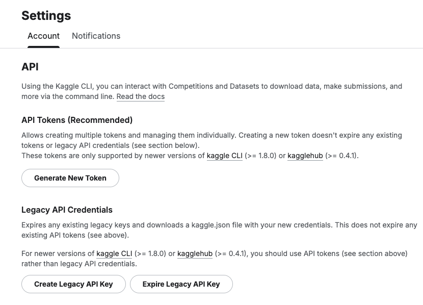
Before we do anything else in the Jupyter Notebook, you will need to log into the Kaggle website and get and API Key Token for your account
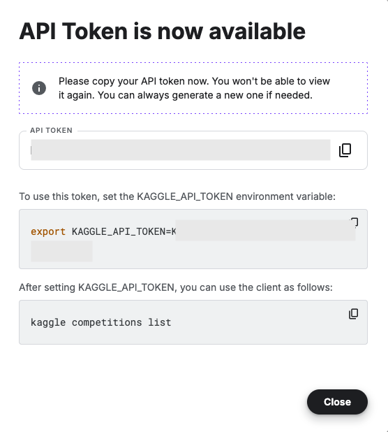
Copy the Kaggle API Key and add it to an environment variable. Here is the code to do this in the Jupyter Notebook.
import osos.environ["KAGGLE_API_TOKEN"] = "..."
You can check that it has been set correctly by running
print(os.environ["KAGGLE_API_TOKEN"])
Now we can get on with accessing the Kaggle datasets. This first approach will use the kaggle python package. With this you can use a mixture of command line commands and package functions
#import kaggle packageimport kaggle#use command line to list the datasets - limited output!kaggle datasets list#use a kaggle package function to list competitionsfrom kaggle.api.kaggle_api_extended import KaggleApiapi = KaggleApi()api.authenticate()api.competitions_list_cli()
I’ve not listed the outputs above, as the output would be very long. I’ll leave that for you to explore.
To download a dataset or all the files for a competion, we can run the following:
#list the files that are part of a competition!kaggle competitions files -c "house-prices-advanced-regression-techniques"name size creationDate --------------------- ---------- -------------------------- data_description.txt 13370 2019-12-15 21:33:35.157000 sample_submission.csv 31939 2019-12-15 21:33:35.224000 test.csv 451405 2019-12-15 21:33:35.212000 train.csv 460676 2019-12-15 21:33:35.259000 #download the competion files!kaggle competitions download -c "house-prices-advanced-regression-techniques"Downloading house-prices-advanced-regression-techniques.zip to /Users/brendan.tierney100%|█████████████████████████████████████████| 199k/199k [00:00<00:00, 714kB/s]
If you get a 403 error when running the above commands, just open the kaggle website and log into your account. Then run again.
The download will create a Zip file on your computer, which you’ll need to unzip.
#!apt-get install unzip!unzip house-prices-advanced-regression-techniques.zip
When unzipped you can now load the dataset into a Pandas dataframe.
import pandas as pd#path to CSV filepath = "train.csv"train_data = pd.read_csv('train.csv')train_data
Or a Spark dataframe.
from pyspark.sql import SparkSession#Create a Spark Sessionspark = SparkSession.builder \ .appName('Kaggle-Data') \ .master('local[*]') \ .getOrCreate()#Spark dataframe - Read CSVdf = spark.read.csv(path)# or if the file has a header record#Spark dataframe - Read CSV with Header df2 = spark.read.option("header", True).csv(path)
An alternative to the above is to use kagglehub package. The download function in this package will download load the files into a local directory
#install kagglehub!pip3 install kagglehubimport kagglehub#download the data fileskagglehub.competition_download('house-prices-advanced-regression-techniques', output_dir='./Kaggle_data', force_download=True)Downloading to ./Kaggle_data/house-prices-advanced-regression-techniques.archive...100%|█████████████████████████████████████████████████████████████████████████████████| 199k/199k [00:00<00:00, 670kB/s]Extracting files...
!ls -l ./Kaggle_datatotal 1888-rw-r--r-- 1 brendan.tierney staff 13370 16 Mar 12:38 data_description.txt-rw-r--r-- 1 brendan.tierney staff 31939 16 Mar 12:38 sample_submission.csv-rw-r--r-- 1 brendan.tierney staff 451405 16 Mar 12:38 test.csv-rw-r--r-- 1 brendan.tierney staff 460676 16 Mar 12:38 train.csv
Exploring Apache Iceberg using PyIceberg – Part 1
Apache Iceberg, an open-source table format that has become the industry standard for data sharing in modern data architectures. In a previous post I explored the core feature of Apache Iceberg and compared it with related technologies such as Apache Hudi and Delta Lake.
In this post we’ll look at some of the inital steps to setup and explore Iceberg tables using Python. I’ll have follow-on posts which will explore more advanced features of Apache Iceberg, again using Python. In this post, we’ll explore the following:
- Environmental setup
- Create an Iceberg Table from a Pandas dataframae
- Explore the Iceberg Table and file system
- Appending data and Time Travel
- Read an Iceberg Table into a Pandas dataframe
- Filtered scans with push-down predicates
Check out the link at the bottom of this post to download the Notebook containing all the PyIceberg code.
Environmental setup
Before we can get started with Apache Iceberg, we need to install it in our environment. I’m going with using Python for these blog posts and that means we need to install PyIceberg. In addition to this package, we also need to install pyiceberg-core. This is needed for some additional feature and optimisations of Iceberg.
pip install "pyiceberg[pyiceberg-core]"
This is a very quick install.
Next we need to do some environmental setup, like importing various packages used in the example code, setuping up some directories on the OS where the Iceberg files will be stored, creating a Catalog and a Namespace.
# Import other packages for this Demo Notebookimport pyarrow as paimport pandas as pdfrom datetime import dateimport osfrom pyiceberg.catalog.sql import SqlCatalog#define location for the WAREHOUSE, where the Iceberg files will be locatedWAREHOUSE = "/Users/brendan.tierney/Dropbox/Iceberg-Demo"#create the directory, True = if already exists, then don't report an erroros.makedirs(WAREHOUSE, exist_ok=True)#create a local Catalogcatalog = SqlCatalog( "local", **{ "uri": f"sqlite:///{WAREHOUSE}/catalog.db", "warehouse": f"file://{WAREHOUSE}", })#create a namespace (a bit like a database schema)NAMESPACE = "sales_db"if NAMESPACE not in [ns[0] for ns in catalog.list_namespaces()]: catalog.create_namespace(NAMESPACE)
That’s the initial setup complete.
Create an Iceberg Table from a Pandas dataframe
We can not start creating tables in Iceberg. To do this, the following code examples will initially create a Pandas dataframe, will convert it from table to columnar format (as the data will be stored in Parquet format in the Iceberg table), and then create and populate the Iceberg table.
#create a Pandas DF with some basic data# Create a sample sales DataFramedf = pd.DataFrame({ "order_id": [1001, 1002, 1003, 1004, 1005], "customer": ["Alice", "Bob", "Carol", "Dave", "Eve"], "product": ["Laptop", "Phone", "Tablet", "Monitor", "Keyboard"], "quantity": [1, 2, 1, 3, 5], "unit_price": [1299.99, 899.00, 549.50, 399.00, 79.99], "order_date": [ date(2024, 1, 15), date(2024, 1, 16), date(2024, 2, 3), date(2024, 2, 20), date(2024, 3, 5)], "region": ["EU", "US", "EU", "APAC", "US"]})# Compute total revenue per orderdf["revenue"] = df["quantity"] * df["unit_price"]print(df)print(df.dtypes) order_id customer product quantity unit_price order_date region \0 1001 Alice Laptop 1 1299.99 2024-01-15 EU 1 1002 Bob Phone 2 899.00 2024-01-16 US 2 1003 Carol Tablet 1 549.50 2024-02-03 EU 3 1004 Dave Monitor 3 399.00 2024-02-20 APAC 4 1005 Eve Keyboard 5 79.99 2024-03-05 US revenue 0 1299.99 1 1798.00 2 549.50 3 1197.00 4 399.95 order_id int64customer objectproduct objectquantity int64unit_price float64order_date objectregion objectrevenue float64dtype: object
That’s the Pandas dataframe created. Now we can convert it to columnar format using PyArrow.
#Convert pandas DataFrame → PyArrow Table # PyIceberg writes via Arrow (columnar format), so this step is requiredarrow_table = pa.Table.from_pandas(df)print("Arrow schema:")print(arrow_table.schema)Arrow schema:order_id: int64customer: stringproduct: stringquantity: int64unit_price: doubleorder_date: date32[day]region: stringrevenue: double-- schema metadata --pandas: '{"index_columns": [{"kind": "range", "name": null, "start": 0, "' + 1180
Now we can define the Iceberg table along with the namespace for it.
#Create an Iceberg table from the Arrow schemaTABLE_NAME = (NAMESPACE, "orders")table = catalog.create_table( TABLE_NAME, schema=arrow_table.schema,)tableorders( 1: order_id: optional long, 2: customer: optional string, 3: product: optional string, 4: quantity: optional long, 5: unit_price: optional double, 6: order_date: optional date, 7: region: optional string, 8: revenue: optional double),partition by: [],sort order: [],snapshot: null
The table has been defined in Iceberg and we can see there are no partitions, snapshots, etc. The Iceberg table doesn’t have any data. We can Append the Arrow table data to the Iceberg table.
#add the data to the tabletable.append(arrow_table)#table.append() adds new data files without overwriting existing ones. #Use table.overwrite() to replace all data in a single atomic operation.
We can look at the file system to see what has beeb written.
print(f"Table written to: {WAREHOUSE}/sales_db/orders/")print(f"Snapshot ID: {table.current_snapshot().snapshot_id}")Table written to: /Users/brendan.tierney/Dropbox/Iceberg-Demo/sales_db/orders/Snapshot ID: 3939796261890602539
Explore the Iceberg Table and File System
And Iceberg Table is just a collection of files on the file system, organised into a set of folders. You can look at these using your file system app, or use a terminal window, or in the examples below are from exploring those directories and files from a Jupyter Notebook.
Let’s start at the Warehouse level. This is the topic level that was declared back when the Environment was being setup. Check that out above in the first section.
!ls -l {WAREHOUSE}-rw-r--r--@ 1 brendan.tierney staff 20480 28 Feb 15:26 catalog.dbdrwxr-xr-x@ 3 brendan.tierney staff 96 28 Feb 12:59 sales_db
We can see the catalog file and a directiory for our ‘sales_db’ namespace. When you explore the contents of this file you will find two directorys. These contain the ‘metadata’ and the ‘data’ files. The following list the files found in the ‘data’ directory containing the data and these are stored in parquet format.
!ls -l {WAREHOUSE}/sales_db/orders/data-rw-r--r--@ 1 brendan.tierney staff 3179 28 Feb 15:22 00000-0-357c029e-b420-459b-8248-b1caf3c030ce.parquet-rw-r--r--@ 1 brendan.tierney staff 3307 28 Feb 15:23 00000-0-3fae55d7-1229-448c-9ffb-ae33c77003a3.parquet-rw-r--r--@ 1 brendan.tierney staff 3179 28 Feb 15:03 00000-0-4ec1ef74-cd24-412e-a35f-bcf3d745bf42.parquet-rw-r--r--@ 1 brendan.tierney staff 3179 28 Feb 15:23 00000-0-984ed6d2-4067-43c4-8c11-5f5a96febd24.parquet-rw-r--r-- 1 brendan.tierney staff 3307 28 Feb 15:26 00000-0-a61264e8-b361-490e-90f7-105a33f20dec.parquet-rw-r--r--@ 1 brendan.tierney staff 3307 28 Feb 15:22 00000-0-ac913dfe-548c-4cb3-99aa-4f1332e02248.parquet-rw-r--r--@ 1 brendan.tierney staff 3307 28 Feb 13:00 00000-0-b3fa23ec-79c6-48da-ba81-ba35f25aa7ad.parquet-rw-r--r--@ 1 brendan.tierney staff 3179 28 Feb 15:25 00000-0-d534a298-adab-4744-baa1-198395cc93bd.parquet-rw-r--r--@ 1 brendan.tierney staff 3307 28 Feb 15:21 00000-0-ef5dd6d8-84c0-4860-828e-86e4e175a9eb.parquet-rw-r--r--@ 1 brendan.tierney staff 3179 28 Feb 15:21 00000-0-f108db1c-39f9-4e2b-b825-3e580cccc808.parquet
I’ll leave you to explore the ‘metadata’ directory.
Read the Iceberg Table back into our Environment
To load an Iceberg table into your environment, you’ll need to load the Catalog and then load the table. We have already have the Catalog setup from a previous step, but tht might not be the case in your typical scenario. The following sets up the Catalog and loads the Iceberg table.
#Re-load the catalog and table (as you would in a new session)catalog = SqlCatalog( "local", **{ "uri": f"sqlite:///{WAREHOUSE}/catalog.db", "warehouse": f"file://{WAREHOUSE}", })table2 = catalog.load_table(("sales_db", "orders"))
When we inspect the structure of the Iceberg table we get the names of the columns and the datatypes.
print("--- Iceberg Schema ---")print(table2.schema())--- Iceberg Schema ---table { 1: order_id: optional long 2: customer: optional string 3: product: optional string 4: quantity: optional long 5: unit_price: optional double 6: order_date: optional date 7: region: optional string 8: revenue: optional double}
An Iceberg table can have many snapshots for version control. As we have only added data to the Iceberg table, we should only have one snapshot.
#Snapshot history print("--- Snapshot History ---")for snap in table2.history(): print(snap)--- Snapshot History ---snapshot_id=3939796261890602539 timestamp_ms=1772292384231
We can also inspect the details of the snapshot.
#Current snapshot metadata snap = table2.current_snapshot()print("--- Current Snapshot ---")print(f" ID: {snap.snapshot_id}")print(f" Operation: {snap.summary.operation}")print(f" Records: {snap.summary.get('total-records')}")print(f" Data files: {snap.summary.get('total-data-files')}")print(f" Size bytes: {snap.summary.get('total-files-size')}")--- Current Snapshot --- ID: 3939796261890602539 Operation: Operation.APPEND Records: 5 Data files: 1 Size bytes: 3307
The above shows use there was 5 records added using an Append operation.
An Iceberg table can be partitioned. When we created this table we didn’t specify a partition key, but in an example in another post I’ll give an example of partitioning this table
#Partition spec & sort order print("--- Partition Spec ---")print(table.spec()) # unpartitioned by default--- Partition Spec ---[]
We can also list the files that contain the data for our Iceberg table.
#List physical data files via scanprint("--- Data Files ---")for task in table.scan().plan_files(): print(f" {task.file.file_path}") print(f" record_count={task.file.record_count}, " f"file_size={task.file.file_size_in_bytes} bytes")--- Data Files --- file:///Users/brendan.tierney/Dropbox/Iceberg-Demo/sales_db/orders/data/00000-0-a61264e8-b361-490e-90f7-105a33f20dec.parquet record_count=5, file_size=3307 bytes
Appending Data and Time Travel
Iceberg tables facilitates changes to the schema and data, and to be able to view the data at different points in time. This is refered to as Time Travel. Let’s have a look at an example of this by adding some additional data to the Iceberg table.
# Get and Save the first snapshot id before writing moresnap_v1 = table.current_snapshot().snapshot_id# New batch of orders - 2 new ordersdf2 = pd.DataFrame({ "order_id": [1006, 1007], "customer": ["Frank", "Grace"], "product": ["Headphones", "Webcam"], "quantity": [2, 1], "unit_price": [249.00, 129.00], "order_date": [date(2024, 4, 1), date(2024, 4, 5)], "region": ["EU", "APAC"], "revenue": [498.00, 129.00],})#Add the datatable.append(pa.Table.from_pandas(df2))
We can list the snapshots.
#Get the new snapshot id and check if different to previoussnap_v2 = table.current_snapshot().snapshot_idprint(f"v1 snapshot: {snap_v1}")print(f"v2 snapshot: {snap_v2}")v1 snapshot: 3939796261890602539v2 snapshot: 8666063993760292894
and we can see how see how many records are in each Snapshot, using Time Travel.
#Time travel: read the ORIGINAL 5-row tabledf_v1 = table.scan(snapshot_id=snap_v1).to_pandas()print(f"Snapshot v1 — {len(df_v1)} rows")#Current snapshot has all 7 rowsdf_v2 = table.scan().to_pandas()print(f"Snapshot v2 — {len(df_v2)} rows")Snapshot v1 — 5 rowsSnapshot v2 — 7 rows
If you inspect the file system, in the data and metadata dirctories, you will notices some additional files.
!ls -l {WAREHOUSE}/sales_db/orders/data!ls -l {WAREHOUSE}/sales_db/orders/metadata
Read an Iceberg Table into a Pandas dataframe
To load the Iceberg table into a Pandas dataframe we can
pd_df = table2.scan().to_pandas()
or we can use the Pandas package fuction
df = pd.read_iceberg("orders", "catalog")
Filtered scans with push-down predicates
PyIceberg provides a fluent scan API. You can read the full table or push down filters, column projections, and row limits — all evaluated at the file level.
Filtered Scan with Push Down Predicates
from pyiceberg.expressions import ( EqualTo, GreaterThanOrEqual, And)# Only EU orders with revenue above €1000df_filtered = ( table2.scan( row_filter=And( EqualTo("region", "EU"), GreaterThanOrEqual("revenue", 1000.0), ) ).to_pandas() )print(df_filtered) order_id customer product quantity unit_price order_date region revenue0 1001 Alice Laptop 1 1299.99 2024-01-15 EU 1299.99
Column Projection – select specific columns
# Only fetch the columns you need — saves I/Odf_slim = ( table2.scan(selected_fields=("order_id", "customer", "revenue")) .to_pandas() )print(df_slim) order_id customer revenue0 1001 Alice 1299.991 1002 Bob 1798.002 1003 Carol 549.503 1004 Dave 1197.004 1005 Eve 399.95
We can also use Arrow for more control.
arrow_result = table2.scan().to_arrow()print(arrow_result.schema)df_from_arrow = arrow_result.to_pandas(timestamp_as_object=True)print(df_from_arrow.head())
order_id: int64
customer: string
product: string
quantity: int64
unit_price: double
order_date: date32[day]
region: string
revenue: double
   order_id customer   product  quantity  unit_price  order_date region  \
0      1001    Alice    Laptop         1     1299.99  2024-01-15     EU
1      1002      Bob     Phone         2      899.00  2024-01-16     US
2      1003    Carol    Tablet         1      549.50  2024-02-03     EU
3      1004     Dave   Monitor         3      399.00  2024-02-20   APAC
4      1005      Eve  Keyboard         5       79.99  2024-03-05     US

   revenue
0  1299.99
1  1798.00
2   549.50
3  1197.00
4   399.95
I’ve put all of the above into a Juputer Notebook. You can download this from here, and you can use it for your explorations of Apache Iceberg.
Check out my next post of Apache Iceberg to see my Python code on explore some additional, and advanced features of Apache Iceberg.
Why Choose Apache Iceberg for Data Interoperability?
Modern data platforms increasingly separate compute from storage, using object stores as durable data lakes while scaling processing engines. Traditional “data lakes” built on Parquet files and Hive-style partitioning have limitations around atomicity, schema evolution, metadata scalability, and multi-engine interoperability. Apache Iceberg addresses these challenges by defining a high-performance table format with transactional guarantees, scalable metadata structures, and engine-agnostic semantics.
Apache Iceberg, an open-source table format that has become the industry standard for data sharing in modern data architectures. Let’s have a look at some of the key features, some of its limitations and a brief look at some of the alternatives.
What is Apache Iceberg and Why Do We Need It? Apache Iceberg is not a storage engine or a compute engine; it’s a table format. It acts as a metadata layer that sits between your physical data files (Parquet, ORC, Avro) and your compute engines.
Before Iceberg, data lakes managed tables as directories of files. To find data, an engine had to list all files in a directory—a slow operation on cloud storage. There was no guarantee of data consistency; a reader might see a partially written file from a running job. Iceberg solves this by tracking individual data files in a persistent tree of metadata. This effectively brings semi-database level reliability, with ACID transactions and snapshot isolation, together with the flexible, low-cost world of object storage.
Iceberg has several important features that bridge the gap between data lakes and traditional warehouses like Oracle:
- ACID Transactions: Iceberg ensures that readers never see partial or uncommitted data. Every write operation creates a new, immutable snapshot. Commits are atomic, meaning they either fully succeed or fully fail. This is the same level of integrity that database administrators have come to expect from Oracle Database for decades.
- Reliable Schema Evolution: In the past, adding or renaming a column in a data lake could require a complete rewrite of your data. Iceberg supports full schema evolution—adding, dropping, updating, or renaming columns—as a metadata operation. It ensures that “zombie” data or schema mismatches never crash your production pipelines.
- Hidden Partitioning: This is a massive usability improvement. Instead of forcing users to know the physical directory structure (e.g.,
WHERE year=2026), Iceberg handles partitioning transparently. You can partition by a timestamp, and Iceberg handles the logic. This makes the data lake feel more like a standard SQL table in a relational Database, where the physical storage details are abstracted away from the analyst. - Time Travel and Rollback: Because Iceberg maintains a history of table snapshots, you can query the data as it existed at any point in history. This is invaluable for auditing, reproducing machine learning models, or quickly rolling back accidental bad writes without needing to restore from a massive tape backup.
While the benefits of Apache Iceberg Tables are critical for its adaption, there are also some limitations:
- Metadata Overhead: The metadata layer adds complexity. For extremely small, high-frequency “single-row” writes, the overhead of managing metadata files can be significant compared to a highly tuned RDBMS.
- Tooling Maturity: While major players like AWS, Snowflake, Oracle, etc have adopted it, support across the entire data ecosystem is still evolving. You may occasionally encounter older tools that don’t natively understand Iceberg tables.
- Write Latency: Every commit involves writing new manifest and metadata files. While this is fine for batch and micro-batch processing, it may not replace the sub-second latency required for OLTP (Online Transactional Processing) workloads where relational Database still reign supreme.
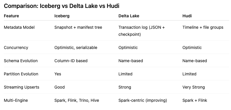
Alternatives to Apache Iceberg tables include Delta Lake (from Databricks) and Apache Hudi. While Delta Lake is highly optimized for the Spark ecosystem and offers a rich feature set, its governance has historically been closely tied to Databricks. Apache Hudi is optimized in streaming ingestion and near-real-time upsert use cases due to its unique indexing and log-merge capabilities. etc it can take some time to consolidate the data change logs. Apache Iceberg is often the choice for organizations seeking maximum interoperability. Its design allows diverse engines, from Spark and Trino to Snowflake and Oracle, to interact with the same data without vendor lock-in and with minimum data copying.
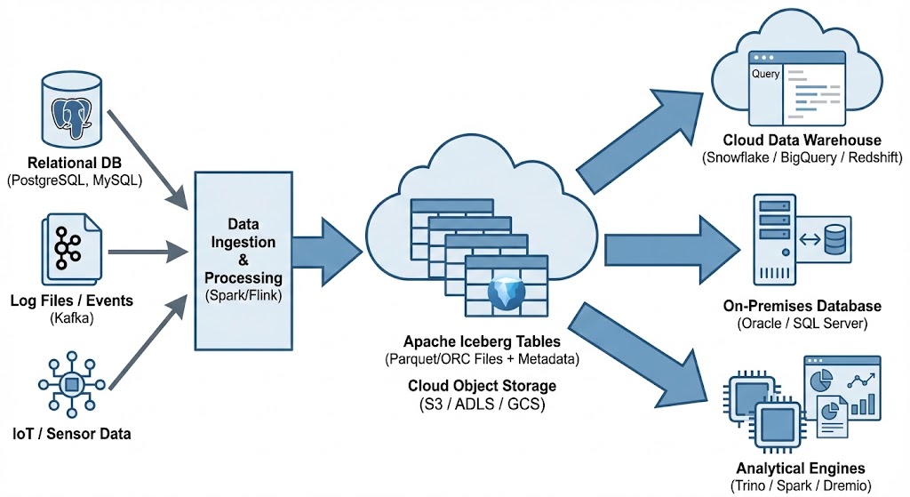
One of Apache Iceberg’s greatest strengths is its ability to act as a central, interoperable layer for data sharing across different platforms. By standardizing on Iceberg, you break down silos. Data ingested once into your data lake becomes immediately available to multiple consuming systems without complex ETL pipelines. Data from various sources is ingested and stored as Apache Iceberg tables in cloud object storage. From there, it can be seamlessly queried by cloud data warehouses like Snowflake and Oracle, etc, and synced to on-premises databases, like Oracle and others, or accessed by various analytical engines for BI and data science.
Using NotebookLM to help with understanding Oracle Analytics Cloud or any other product
Over the past few months, we’ve seen a plethora of new LLM related products/agents being released. One such one is NotebookLM from Google. The offical description say “NotebookLM is an AI-powered research and note-taking tool from Google Labs that allows users to ground a large language model (like Gemini) in their own documents, such as PDFs, Google Docs, website URLs, or audio, acting as a personal, intelligent research assistant. It facilitates summarizing, analyzing, and querying information within these specific sources to create study guides, outlines, and, notably, “Audio Overviews” (podcast-style summaries)”
Let’s have a look at using NotebookLM to help with answering questions and how it can help with understanding Oracle Analytics Cloud (OAC).

Yes, you’ll need a Google account, and Yes you need to be OK with uploading your documents to NotebookLM. Make sure you are not breaking any laws (IP, GDPR, etc). It’s really easy to create your first notebook. Simply click on ‘Create new notebook’.
When the notebook opens, you can add your documents and webpages to the notebook. These can be documents in PDF, audio, text, etc to the notebook repository. Currently, there seems to be a limit of 50 documents and webpages that can be added.
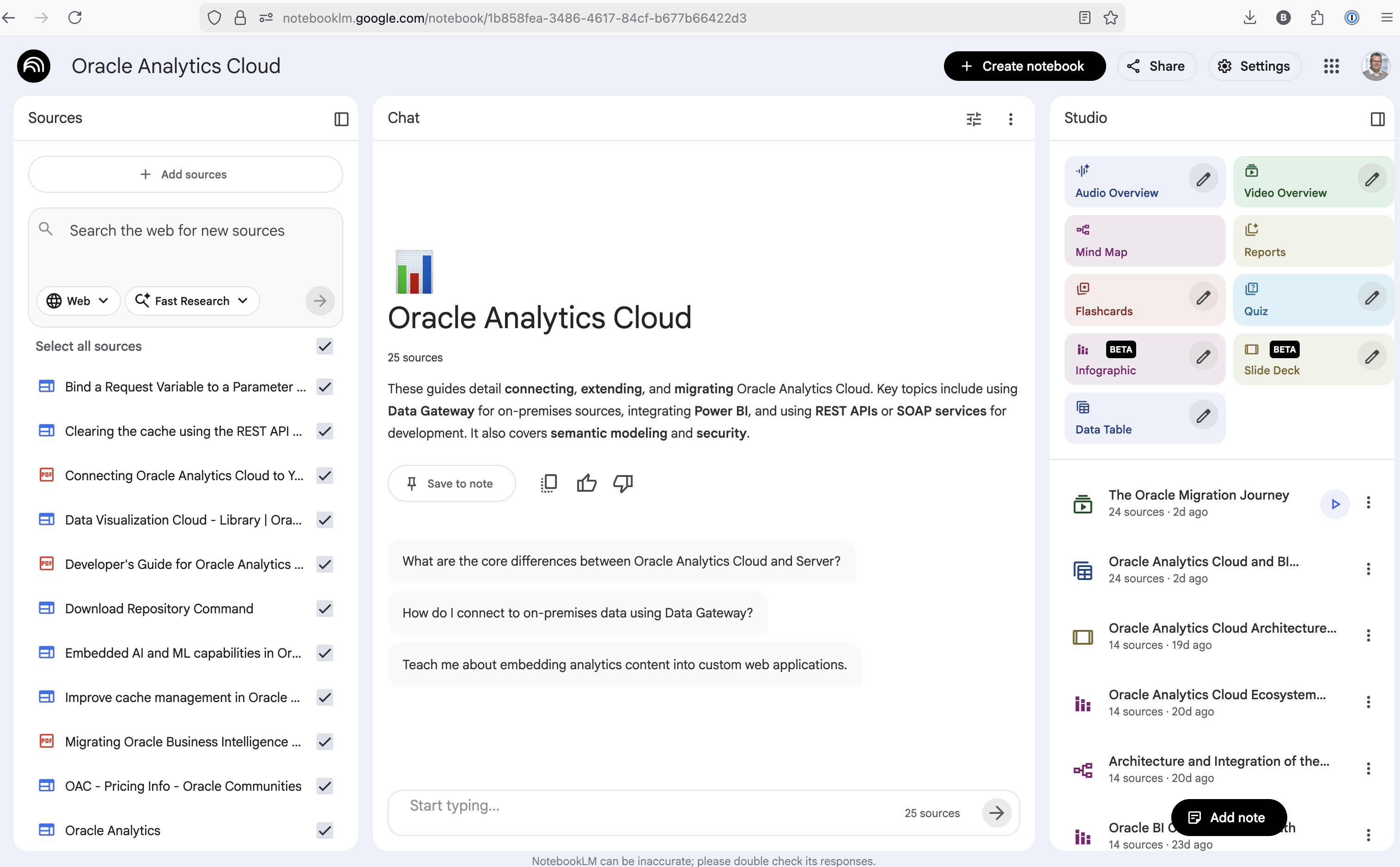
The main part of the NotebookLM provides a chatbot where you can ask questions, and the NotebookLM will search through the documents and webpages to formulate an answer. In addition to this, there are features that allow you to generate Audio Overview, Video Overview, Mind Map, Reports, Flashcards, Quiz, Infographic, Slide Deck and a Data Table.
Before we look at some of these and what they have created for Oracle Analytics Cloud, there is a small warning. Some of these can take a long time to complete, that is, if they complete. I’ve had to run some of these features multiple times to get them to create. I’ve run all of the features, and the output from these can be seen on the right-hand side of the above image.
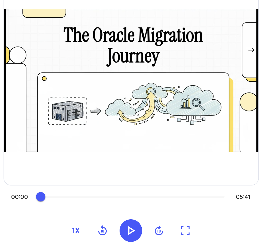
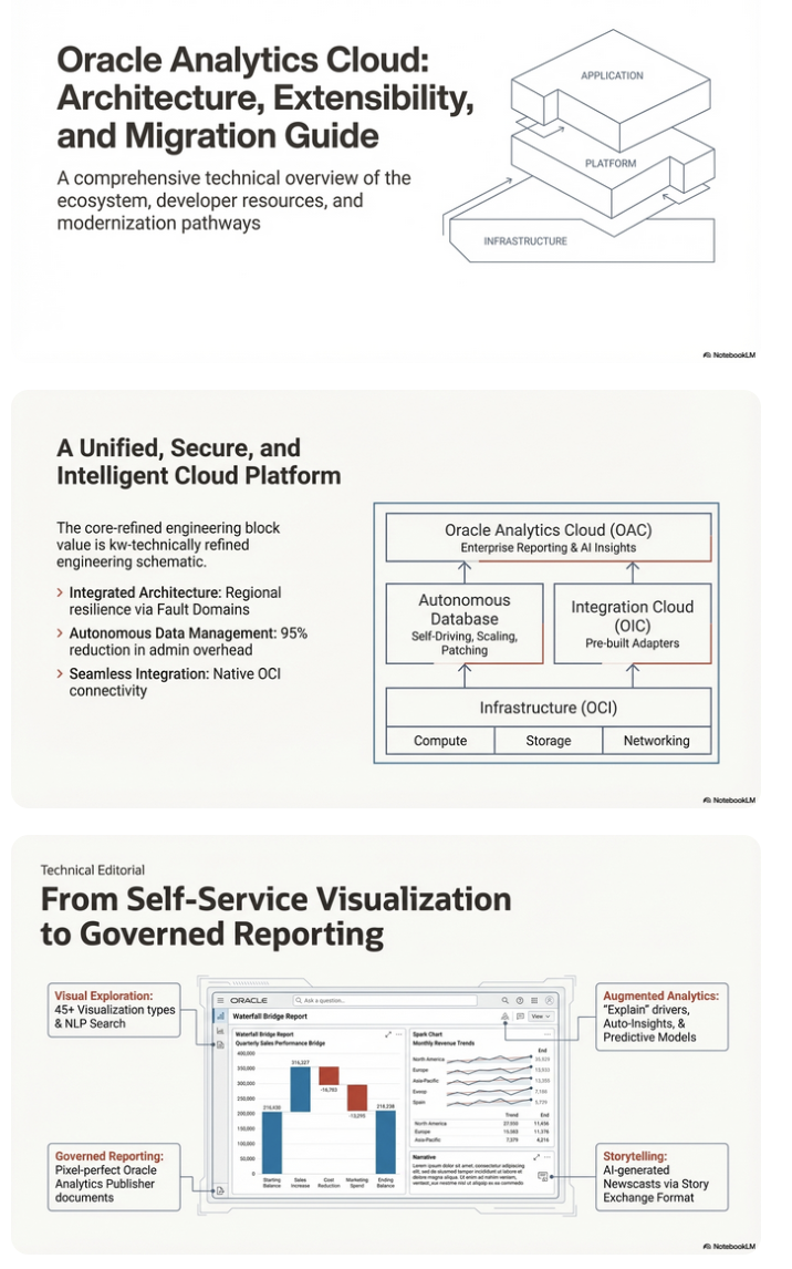
It created a 15-slide presentation on Oracle Analytics Cloud and its various features, and a five minute video on migrating OAC.
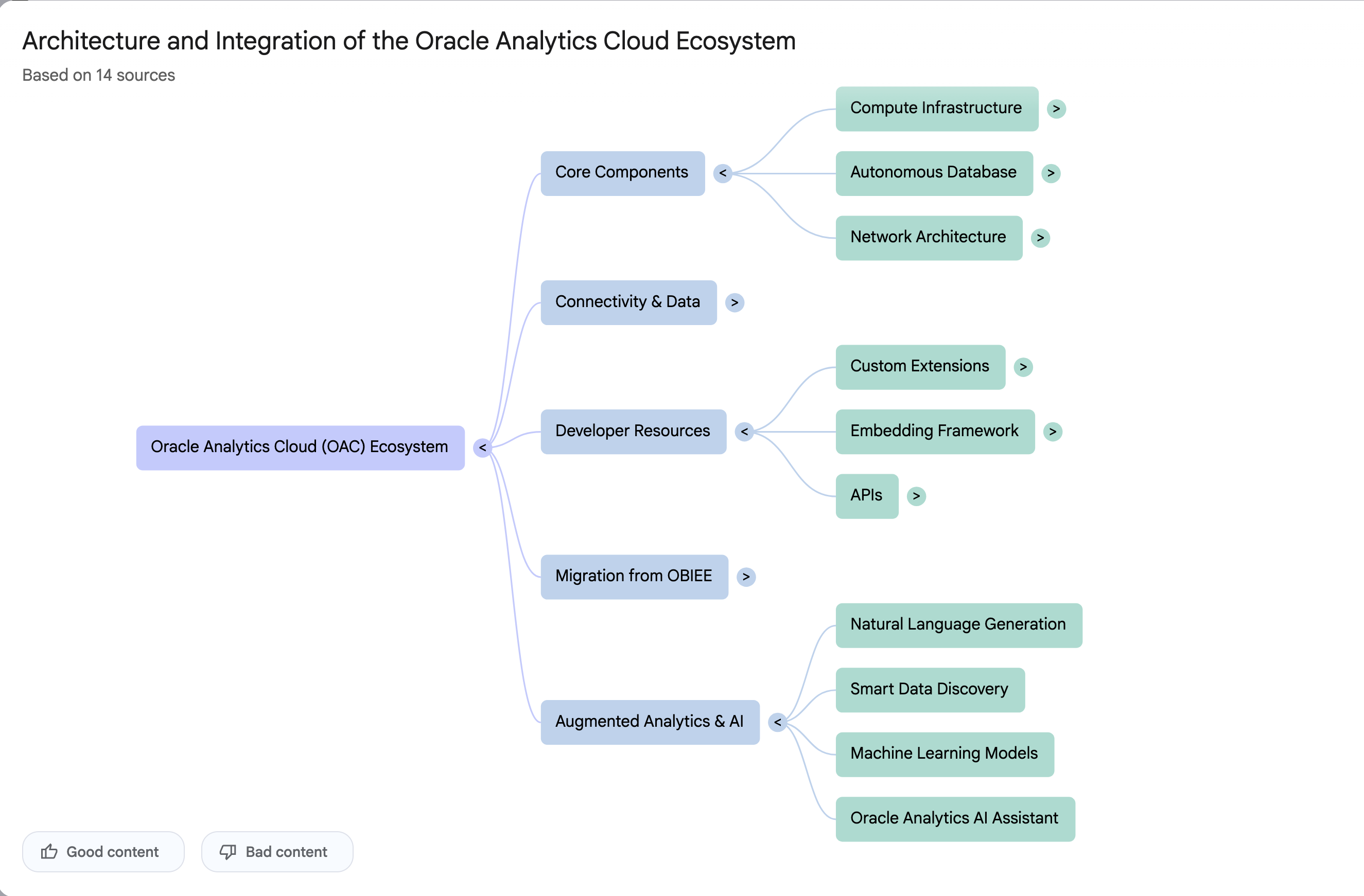
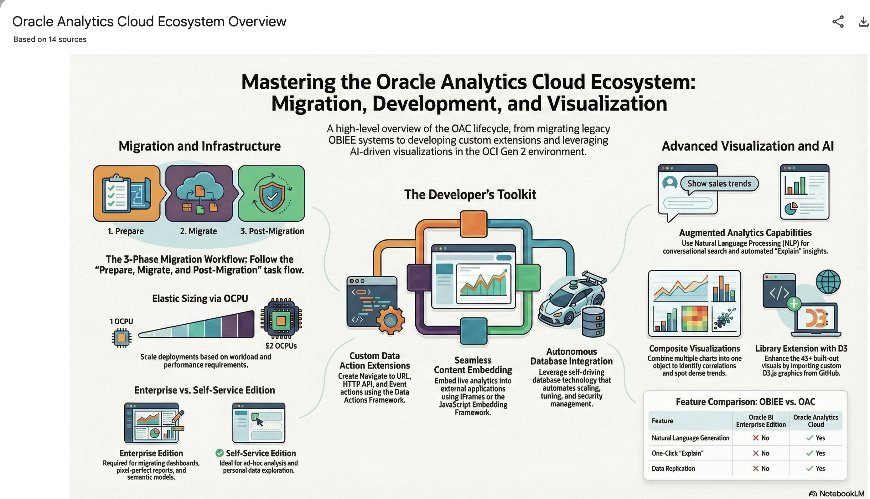
It also created a Mind-map, and an Infographic.
Handling Multi-Column Indexes in Pandas Dataframes
It’s a little annoying when an API changes the structure of the data it returns and you end up with your code breaking. In my case, I experienced it when a dataframe having a single column index went to having a multi-column index. This was a new experience for me, at this time, as I hadn’t really come across it before. The following illustrates one particular case similar (not the same) that you might encounter. In this test/demo scenario I’ll be using the yfinance API to illustrate how you can remove the multi-column index and go back to having a single column index.
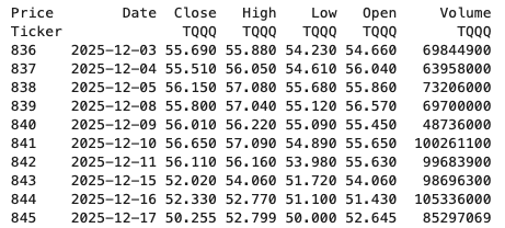
In this demo scenario, we are using yfinance to get data on various stocks. After the data is downloaded we get something like this.
The first step is to do some re-organisation.
df = data.stack(level="Ticker", future_stack=True)
df.index.names = ["Date", "Symbol"]
df = df[["Open", "High", "Low", "Close", "Volume"]]
df = df.swaplevel(0, 1)
df = df.sort_index()
df
This gives us the data in the following format.
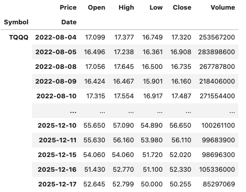
The final part is to extract the data we want by applying a filter.
df.xs(“TQQQ”)
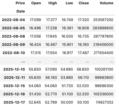
And there we have it.
As I said at the beginning the example above is just to illustrate what you can do.
If this was a real work example of using yfinance, I could just change a parameter setting in the download function, to not use multi_level_index.
data = yf.download(t, start=s_date, interval=time_interval, progress=False, multi_level_index=False)

You must be logged in to post a comment.