
OML
How to access and use Multilingual embedding models using OML for Python 2.1
With the release of OML for Python 2.1, we have a newer approach for accessing and generating embedding models in ONNX format (from Hugging Face), which can then be loaded into the Database (>=23.7ai). Although with this newer approach, we need to be aware of the previous way of doing it (<=23.6). As of 23.7ai this previous approach is now deprecated. Given the short time the previous approach was around, things could yet change with subsequent releases.
As the popularity of Vector Search spreads, there have been some challenges relating to obtaining and using suitable models within a Database. Oracle 23ai introduced the ability to load an embedding model in ONNX format into the database. These could be easily used to create and update embedding vectors for your data. But there were some limitations and challenges with what ONNX models could be used, and sometimes this was limited to the formatting of the ONNX metadata and the pretrained models themselves.
To ease the process of locating, converting and loading an embedding model into an Oracle Database, Oracle Machine Learning for Python 2.1 has been released with some new features and methods to make the process slightly easier. There are three constraints for doing this: 1) you need to use Oracle Machine Learning for Python 2.1 (OML4Py 2.1), and 2) you need to use Oracle 23.7ai (or greater) Database (This later requirement is to allow for the expanded range of embedding models) and 3) Python 3.12 (or greater).
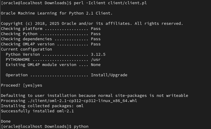
There are a few additional Python libraries needed, so check the documentation for more details on what the most recent version of these should be. But do be careful of the documentation as the version I followed there was some inconsistencies in different sections regarding the requirements and steps to follow for installation. Hopefully this will be tidied up by the time you read the documentation.
With OML4Py 2.1 there is a class called oml.utils.onnxpipeline, with a number of methods to support the exploration of preconfigured models. These include: from_preconfigured(), from_template() and show_preconfigured(). This last one displays the list of preconfigured models.
oml.ONNXPipelineConfig.show_preconfigured()
['sentence-transformers/all-mpnet-base-v2', 'sentence-transformers/all-MiniLM-L6-v2', 'sentence-transformers/multi-qa-MiniLM-L6-cos-v1', 'sentence-transformers/distiluse-base-multilingual-cased-v2', 'sentence-transformers/all-MiniLM-L12-v2', 'BAAI/bge-small-en-v1.5', 'BAAI/bge-base-en-v1.5', 'taylorAI/bge-micro-v2', 'intfloat/e5-small-v2', 'intfloat/e5-base-v2', 'thenlper/gte-base', 'thenlper/gte-small', 'TaylorAI/gte-tiny', 'sentence-transformers/paraphrase-multilingual-mpnet-base-v2', 'intfloat/multilingual-e5-base', 'intfloat/multilingual-e5-small', 'sentence-transformers/stsb-xlm-r-multilingual', 'Snowflake/snowflake-arctic-embed-xs', 'Snowflake/snowflake-arctic-embed-s', 'Snowflake/snowflake-arctic-embed-m', 'mixedbread-ai/mxbai-embed-large-v1', 'openai/clip-vit-large-patch14', 'google/vit-base-patch16-224', 'microsoft/resnet-18', 'microsoft/resnet-50', 'WinKawaks/vit-tiny-patch16-224', 'Falconsai/nsfw_image_detection', 'WinKawaks/vit-small-patch16-224', 'nateraw/vit-age-classifier', 'rizvandwiki/gender-classification', 'AdamCodd/vit-base-nsfw-detector', 'trpakov/vit-face-expression', 'BAAI/bge-reranker-base']
We can inspect the full details of all models or for an individual model by changing some of the parameters.
oml.ONNXPipelineConfig.show_preconfigured(include_properties=True, model_name='microsoft/resnet-50')
[{'checksum': 'fca7567354d0cb0b7258a44810150f7c1abf8e955cff9320b043c0554ba81f8e', 'model_type': 'IMAGE_CONVNEXT', 'pre_processors_img': [{'name': 'DecodeImage', 'do_convert_rgb': True}, {'name': 'Resize', 'enable': True, 'size': {'height': 384, 'width': 384}, 'resample': 'bilinear'}, {'name': 'Rescale', 'enable': True, 'rescale_factor': 0.00392156862}, {'name': 'Normalize', 'enable': True, 'image_mean': 'IMAGENET_STANDARD_MEAN', 'image_std': 'IMAGENET_STANDARD_STD'}, {'name': 'OrderChannels', 'order': 'CHW'}], 'post_processors_img': []}]
Let’s prepare a preconfigured model using the simplest approach. In this example we’ll use the 'sentence-transformers/multi-qa-MiniLM-L6-cos-v1' model. Start by defining a pipeline.
pipeline = oml.utils.ONNXPipeline(model_name="sentence-transformers/multi-qa-MiniLM-L6-cos-v1")We now have the choice of loading it straight to your database using an already established OML connection.
pipeline.export2db("my_onnx_model_db")or you can export the model to a file
pipeline.export2file("my_onnx_model", output_dir="/home/oracle/onnx")
When you check the file system, you’ll see something like the following. Depending on the model you exported and any configuration changes to the model, the file size will vary in size.
-rw-r--r--. 1 oracle oracle 90636512 Apr 22 12:00 my_onnx_model.onnxIs you ran the export2file() function you’ll need to move that file to the database server. This will involve talking gently with the DBA to get their assistance. Once permission is obtained from the DBA, the ONNX file will be copied into a directory that is referenced from within the database. This is a simple task of defining an external file system directory where the file is located. In the example below the directory is referenced as ONNX_DIR. This is the reference defined in the database, which has a pointer to directory on the file system. The next task is to load the ONNX file into your Database schema.
BEGIN
   DBMS_VECTOR.LOAD_ONNX_MODEL(
        directory => 'ONNX_DIR',
        file_name => 'my_onnx_model.onnx',
        model_name => 'Multi-qa-MiniLM-L6-Cos-v1');
END;
Once loaded the model can be used to create Vector Embeddings.
OML4Py – AutoML – Step-by-Step Approach
Automated Machine Learning (AutoML) is or was a bit of a hot topic over the past couple of years. With various analysis companies like Gartner and others pushing for the need for AutoML, lots and lots of vendors have been creating different types of offerings to support this.
I’ve written some blog posts about AutoML already, from describing what it is and the different types, to showing how to do a black box approach using Oracle OML4Py, and also for using Oracle Machine Learning (OML) AutoML UI. Go check out those posts. In this post I will look at the more detailed step-by-step approach to AutoML using OML4Py. The same data set and cloud account/setup will be used. This will make it easier for you to compare the steps, the results and the AutoML experience across the different OML offerings.
Check out my previous post where I give details of the data set and some data preparation. I won’t repeat those here, but will move onto performing the step-by-step AutoML using OML4Py. The following diagram, from Oracle, outlines the steps involved

A little reminder/warning before you use AutoML in OML4Py. It only works for Classification (binary and multi-class) and Regression problems. The following code example illustrates a binary class problem, but in general there is no difference between the each type of Classification and Regression, except for the evaluation metrics, which I will list below.
Step 1 – Prepare the Data Set & Setup
See my previous blog post where I prepare the data set. I’m not going to repeat those steps here to save a little bit of space.
Also have a look at what libraries to load/import.
Step 2 – Automatic Algorithm Selection
The first step to configure and complete is select the “best model” from a selection of available Algorithms. Not all of the in-database algorithms are available to use in AutoML, which is a pity as there are some algorithms that can produce really accurate model. Hopefully with time these will be added.
The function to use is called AlgorithmSelection. This consists of two parts. The first is to define the parameters and the second part is to run it. This function accepts three parameters:
- mining function : ‘classification’ or ‘regression. Classification can be for binary and multi-class.
- score metric : the evaluation metric to evaluate the model performance. The following list gives the evaluation metric for each mining function
binary classification – accuracy (default), f1, precision, recall, roc_auc, f1_micro, f1_macro, f1_weighted, recall_micro, recall_macro, recall_weighted, precision_micro, precision_macro, precision_weighted
multiclass classification – accuracy (default), f1_micro, f1_macro, f1_weighted, recall_micro, recall_macro, recall_weighted, precision_micro, precision_macro, precision_weighted
regression – r2 (default), neg_mean_squared_error, neg_mean_absolute_error, neg_mean_squared_log_error, neg_median_absolute_error
- parallel : degree of parallelism to use. Default it system determined.
The second step uses this configuration and runs the code to find the “best models”. This takes the training data set (in typical Python format), and can also have a number of additional parameters. See my previous blog post for a full list of these, but ignore adaptive sampling. To keep life simple, you only really need to use ‘k’ and ‘cv’. ‘k’ specifies the number of models to include in the return list, default is 3. ‘cv’ tells how many levels of cross validation to perform. To keep things consistent across these blog posts and make comparison easier, I’m going to set ‘cv=5’
as_bank = automl.AlgorithmSelection(mining_function='classification',
                                    score_metric='accuracy', parallel=4)
oml_bank_ms = as_bank.select(oml_bank_X, oml_bank_y, cv=5)
To display the results and select out the best algorithm:
print("Ranked algorithms with Evaluation score:\n", oml_bank_ms)
selected_oml_bank_ms = next(iter(dict(oml_bank_ms).keys()))
print("Best algorithm =", selected_oml_bank_ms)

Ranked algorithms with Evaluation score:
 [('glm', 0.8668130990415336), ('glm_ridge', 0.8668130990415336), ('nb', 0.8634185303514377)]
Best algorithm = glm
This last bit of code is import, where the “best” algorithm is extracted from the list. This will be used in the next step.
“It Depends” is a phrase we hear/use a lot in IT, and the same applies to using AutoML. The model returned above does not mean it is the “best model”. It Depends on the parameters used, primarily the Evaluation Metric, but also the number set for CV (cross validation). Here are some examples of changing these and their results. As you can see we get a slightly different set of results or “best model” for each. My advice is to set ‘k’ large (eg current maximum values is 8), as this will ensure all algorithms are evaluated and not just a subset of them (potential hard coded ordered list of algorithms)
oml_bank_ms5 = as_bank.select(oml_bank_X, oml_bank_y, k=5)
oml_bank_ms5

[('glm', 0.8668130990415336), ('glm_ridge', 0.8668130990415336), ('nb', 0.8634185303514377), ('rf', 0.862020766773163), ('svm_linear', 0.8552316293929713)]
oml_bank_ms10 = as_bank.select(oml_bank_X, oml_bank_y, k=10)
oml_bank_ms10

[('glm', 0.8668130990415336), ('glm_ridge', 0.8668130990415336), ('nb', 0.8634185303514377), ('rf', 0.862020766773163), ('svm_linear', 0.8552316293929713), ('nn', 0.8496405750798722), ('svm_gaussian', 0.8454472843450479), ('dt', 0.8386581469648562)]
Here are some examples when the Score Metric is changed, and the impact it can have.
as_bank2 = automl.AlgorithmSelection(mining_function='classification',
                                     score_metric='f1', parallel=4)

oml_bank_ms2 = as_bank2.select(oml_bank_X, oml_bank_y, k=10)
oml_bank_ms2

[('rf', 0.6163242642976126), ('glm', 0.6160046056419113), ('glm_ridge', 0.6160046056419113), ('svm_linear', 0.5996686913307566), ('nn', 0.5896457765667574), ('svm_gaussian', 0.5829741379310345), ('dt', 0.5747368421052631), ('nb', 0.5269709543568464)]
as_bank3 = automl.AlgorithmSelection(mining_function='classification',
                                     score_metric='f1', parallel=4)

oml_bank_ms3 = as_bank3.select(oml_bank_X, oml_bank_y, k=10, cv=2)
oml_bank_ms3

[('glm', 0.60365647055431), ('glm_ridge', 0.6034077555816686), ('rf', 0.5990036646816308), ('svm_linear', 0.588201766334537), ('svm_gaussian', 0.5845019676714007), ('nn', 0.5842357537014313), ('dt', 0.5686862482989511), ('nb', 0.4981168003466766)]
as_bank4 = automl.AlgorithmSelection(mining_function='classification',
                                     score_metric='f1', parallel=4)

oml_bank_ms4 = as_bank4.select(oml_bank_X, oml_bank_y, k=10, cv=5)
oml_bank_ms4

[('glm', 0.583504644833276), ('glm_ridge', 0.58343736244422), ('rf', 0.5815952044164737), ('svm_linear', 0.5668069231027809), ('nn', 0.5628153929281711), ('svm_gaussian', 0.5613976370223811), ('dt', 0.5602129668741175), ('nb', 0.49153999668083814)]
The problem we now have with AutoML, it is telling us different answers for “best model”. To most that might be confusing but for the more technical data scientist they will know why. In very very simple terms, you are doing different things with the data and because of this you can get a different answer.
It is because of these different possible answers answers for the “best model”, is the reason AutoML can really only be used as a guide (a pointer towards what might be the “best model”), and cannot be relied upon to give a “best model”. AutoML is still not suitable for the general data analyst despite what some companies are saying.
Lots more could be discussed here but let’s more onto the next step.
Step 3 – Automatic Feature Selection
In the previous steps we have identified a possible “best model”. Let’s pretend the “best model” is the “best model”. The next steps is to look at how this model can be refined and improved using a subset of the features/attributes/columns. FeatureSelection looks are examining the data when combined with the model to find the optimised set of features/attributes/columns, to improve the model performance i.e. make it more accurate or have a better outcome based on the evaluation or score metric. For simplicity I’m going to use the result from the first example produced in the previous step. In a similar way to Step 2, there are two parts to setup and run the Feature Selection (Reduction). Each part is setup in a similar way to Step 2, with the parameters for FeatureSelection being the same values as those used for AlgorithmSelection. For the ‘reduce’ function, pass in the name of the “best model” or “best algorithm” from Step 2. This was extracted to a variable called ‘selected_oml_bank_ms’. Most of the other parameters the ‘reduce’ function takes are similar to the ‘select’ function. Again keeping things consistent, pass in the training data set and set the number of cross validations to 5.
fs_oml_bank = automl.FeatureSelection(mining_function = 'classification',
                                      score_metric = 'accuracy', parallel=4)

oml_bank_fsR = fs_oml_bank.reduce(selected_oml_bank_ms, oml_bank_X, oml_bank_y, cv=5)
We can now look at the results from this listing the reduced set of features/columns and comparing the number of features/columns in the original data set to the reduced set.
#print(oml_bank_fsR)
oml_bank_fsR_l = oml_bank_X[:,oml_bank_fsR]

print("Selected columns:", oml_bank_fsR_l.columns)
print("Number of columns:")
"{} reduced to {}".format(len(oml_bank_X.columns), len(oml_bank_fsR_l.columns))


Selected columns: ['DURATION', 'PDAYS', 'EMP_VAR_RATE', 'CONS_PRICE_IDX', 'CONS_CONF_IDX', 'EURIBOR3M', 'NR_EMPLOYED']
Number of columns:
'20 reduced to 7'
In this example the data set gets reduced from having 20 features/columns in the original data set, down to having 7 features/columns.
Step 4 – Automatic Model Tuning
Up to now, we have identified the “best model” / “best algorithm” and the optimised reduced set of features to use. The final step is to take the details generated from the previous steps and use this to generate a Tuned Model. In a similar way to the previous steps, this involve two parts. The first sets up some parameters and the second runs the Model Tuning function called ‘tune’. Make sure to include the data frame containing the reduced set of features/attributes.
mt_oml_bank = automl.ModelTuning(mining_function='classification', score_metric='accuracy', parallel=4)

oml_bank_mt = mt_oml_bank.tune(selected_oml_bank_ms, oml_bank_fsR_l, oml_bank_y, cv=5)

print(oml_bank_mt)
The output is very long and contains the name of the Algorithm, the hyperparameters used for the final model, the features used, and (at the end) lists the various combinations of hyperparameters used and the evaluation metric score for each combination. Partial output shown below.
mt_oml_bank = automl.ModelTuning(mining_function='classification', score_metric='accuracy', parallel=4)

oml_bank_mt = mt_oml_bank.tune(selected_oml_bank_ms, oml_bank_fsR_l, oml_bank_y, cv=5)
print(oml_bank_mt)

{'best_model':
Algorithm Name: Generalized Linear Model

Mining Function: CLASSIFICATION

Target: TARGET_Y

Settings:
setting name setting value
0 ALGO_NAME ALGO_GENERALIZED_LINEAR_MODEL
1 CLAS_WEIGHTS_BALANCED OFF
...
...
, 'all_evals': [(0.8544108809341562, {'CLAS_WEIGHTS_BALANCED': 'OFF', 'GLMS_NUM_ITERATIONS': 30, 'GLMS_SOLVER': 'GLMS_SOLVER_CHOL'}), (0.8544108809341562, {'CLAS_WEIGHTS_BALANCED': 'ON', 'GLMS_NUM_ITERATIONS': 30, 'GLMS_SOLVER': 'GLMS_SOLVER_CHOL'}), (0.8544108809341562, {'CLAS_WEIGHTS_BALANCED': 'OFF', 'GLMS_NUM_ITERATIONS': 31, 'GLMS_SOLVER': 'GLMS_SOLVER_CHOL'}), (0.8544108809341562, {'CLAS_WEIGHTS_BALANCED': 'OFF', 'GLMS_NUM_ITERATIONS': 173, 'GLMS_SOLVER': 'GLMS_SOLVER_CHOL'}), (0.8544108809341562, {'CLAS_WEIGHTS_BALANCED': 'OFF', 'GLMS_NUM_ITERATIONS': 174, 'GLMS_SOLVER': 'GLMS_SOLVER_CHOL'}), (0.8544108809341562, {'CLAS_WEIGHTS_BALANCED': 'OFF', 'GLMS_NUM_ITERATIONS': 337, 'GLMS_SOLVER': 'GLMS_SOLVER_CHOL'}), (0.8544108809341562, {'CLAS_WEIGHTS_BALANCED': 'OFF', 'GLMS_NUM_ITERATIONS': 338, 'GLMS_SOLVER': 'GLMS_SOLVER_CHOL'}), (0.8544108809341562, {'CLAS_WEIGHTS_BALANCED': 'ON', 'GLMS_NUM_ITERATIONS': 10, 'GLMS_SOLVER': 'GLMS_SOLVER_CHOL'}), (0.8544108809341562, {'CLAS_WEIGHTS_BALANCED': 'ON', 'GLMS_NUM_ITERATIONS': 173, 'GLMS_SOLVER': 'GLMS_SOLVER_CHOL'}), (0.8544108809341562, {'CLAS_WEIGHTS_BALANCED': 'ON', 'GLMS_NUM_ITERATIONS': 174, 'GLMS_SOLVER': 'GLMS_SOLVER_CHOL'}), (0.8544108809341562, {'CLAS_WEIGHTS_BALANCED': 'ON', 'GLMS_NUM_ITERATIONS': 337, 'GLMS_SOLVER': 'GLMS_SOLVER_CHOL'}), (0.8544108809341562, {'CLAS_WEIGHTS_BALANCED': 'ON', 'GLMS_NUM_ITERATIONS': 338, 'GLMS_SOLVER': 'GLMS_SOLVER_CHOL'}), (0.4211156437080018, {'CLAS_WEIGHTS_BALANCED': 'ON', 'GLMS_NUM_ITERATIONS': 10, 'GLMS_SOLVER': 'GLMS_SOLVER_SGD'}), (0.11374128955112069, {'CLAS_WEIGHTS_BALANCED': 'OFF', 'GLMS_NUM_ITERATIONS': 30, 'GLMS_SOLVER': 'GLMS_SOLVER_SGD'}), (0.11374128955112069, {'CLAS_WEIGHTS_BALANCED': 'ON', 'GLMS_NUM_ITERATIONS': 30, 'GLMS_SOLVER': 'GLMS_SOLVER_SGD'})]}
The list of parameter settings and the evaluation score is an ordered list in decending order, starting with the best model.
We can extract the different parts of this dictionary object by using the following:
#display the main model details
print(oml_bank_mt['best_model'])
Now extract the evaluation metric score and the parameter settings used for the best model, (position 0 of the dictionary)
score, params = oml_bank_mt['all_evals'][0]
And that’s it, job done with using OML4Py AutoML to generate an optimised model.
The example above is for a Classification problem. If you had a Regression problem all you need to do is replace ‘classification’ with ‘regression’, and change the score_metric parameter to ‘r2’, or one of the other Regression metric values (see above for list of these.
OML4Py – AutoML – An Example
OML4Py (Oracle Machine Learning for Python) is Oracle’s offering where you can use Python commands to process and analyse data in an Oracle Database without having to write any SQL. OML4Py, via it’s transparency layer, translates Python code into SQL, executes it in the Database and then presents the results back to you in your Python environment. The examples shown in this post used the OML Notebooks available with Autonomous Databases on Oracle Cloud.
[Warning: the functionality available with initial release of OML4Py is very limited and may not suit most Python developers. Hopefully this will be addressed in later releases]
One of the features of OML4Py is Automated Machine Leaning (AutoML). At some point in the near future Oracle will have a GUI interface for AutoML, which will save you from having to write any code, such as the example in this post. See my previous blog post about AutoML. It is a general discussion on AutoML and some things you need to be careful with. Also, be careful of the marketing around AutoML from all vendors. The reality doesn’t necessarily live up to marketing

OML4Py has a couple of approaches you can follow to Automatically generate a Machine Learning Model (see previous blog post). The first of these can be considered the Black Box approach for AutoML, and the example below illustrates an example of this. The more detailed version of AutoML will be covered in a later post.
[Info: I’m using Oracle Free Tier Database. At time of writing this post OML4Py is only available with Oracle Autonomous 19c]
But before look at these, the first step we need to do is setup the data set to use for AutoML. I’ll be using the popular Portuguese Bank data set. Each code snippets shown below are for a one cell in my OML Notebooks. The data set exists as a table in my schema called BANK_ADDITIONAL_FULL. The sync command creates a proxy object in the notebook session pointing to the table in the DB. No data is copied into the notebook.
%python
import oml
from oml import automl
import pandas as pd
%python
oml_bank = oml.sync(table = 'BANK_ADDITIONAL_FULL')
type(oml_bank)
Let’s explore the data. Remember the data lives in a table in the DB and only the results are displayed
%python
oml_bank.head()

%python
oml_bank.describe()

Now remove one attribute from data set and at the sample time setup the dataframes for input to the ML. This is highly correlated to the the target variable.
%python
oml_bank_X, oml_bank_y = oml_bank.drop('TARGET_Y'), oml_bank['TARGET_Y']
Finally, we can now look at the first of the AutoML options, the black box option. This uses the AutoML ModelSelection function. Using this you can define the type of machine learning to perform (‘classification) and set some additional parameters. The parallel parameter will probably not have too much of an effect when using the Oracle Free Tier, but will certainly improved performance when using additional compute resources.
The example below is very simple and the setup of it is very simple. The ModelSelection function sets up the parameters for the AutoML to function. The ‘select’ function runs the AutoML based on those parameters along with some additional ones. These parameters and the additional ones available are explained below, after this first example.
%python
ms_bank = automl.ModelSelection(mining_function='classification', parallel=4)
ModelSelection can have the following parameters. The possible values for each are listed with the value in bold being the default value:
- mining_function : the type of ML to preform, only two option available for this, classification or regression
- score_metric: what metric to use for evaluating the models. Defaults for binary and multi classification balanced_accuracy is used and default for regression is neg_mean_squared_error. Other options for regression include r2, neg_mean_absolute_error and neg_median_absolute_error. For classification other options include, accuracy, f1, precision, recall, roc_auc, f1_micro, f1_macro, f1_weighted, recall_micro, recall_macro, recall_weighted, precision_micro, precision_macro, precision_weighted
- parallel: degree of parallelism to use, None or a number.
Having defined ModelSelection settings, we can move onto using it to preform (black box) AutoML, using the ‘select’ function. Oracle doesn’t tell us what it does inside this black box except that it uses ML and meta-learning techniques to work out which algorithms to use, what subsets of the original data set to use to give use a optimal outcome. It’s there secret recipe!
The ‘select’ function elevates all the available algorithms, creating models for each or a subset of them based on the meta-learning, and returns the “best” one. The function returns just one model, which is the “best”. The value set for ‘k’ tells the function how many of the “best” or top models created, how many of these to tune before returning the “best” one.
Now, let’s run an example of the ‘select’ function and what parameters is can have
- X: input data set consisting of the columns to use for Training.
- y: the column containing the Target variable.
- case_id: columns name of case_id, default is None. If supplied can be used for data sampling
- k: the number of (best) models to tune. Default is 3, but can be set to any number between one and eight, as setting it higher than that has no effect as there aren’t any more than that number of algorithms in the database!
- solver: allowed values are fast (default) and exhaustive. fast uses internal ML and meta-learning thereby reducing the search space. exhaustive will be slower as it will evaluate all algorithms and options for creating a model.
- cv: cross validation. Default is auto, but can be set to a number or set to None uses inputs defined in X_valid and y_valid defined below. auto will determine the number based on size of input data set, and when a number is provided will perform that number cross validation.
- adaptive_sampling: use adaptive sampling to reduce data set size to speed up runtime of ‘select’ function. Default is True, otherwise use False.
- X_valid: validation data set, default is None.
- y_valid: validation target column, default is None.
- time_budget: defines a time constraint on how how long, in seconds, to spend working out the solution. Default is None, or number for number of seconds. Useful for large data sets or for when you need a quicker results, and can be increased based on experimentation.
Here is a basic example of using the ‘select’ function, using the data frames created above as input, ‘k’ is set to five telling the function to tune the top five models created based on doing five fold cross-validation ‘cv’.
best_model = ms_bank.select(oml_bank_X, oml_bank_y, k=5, cv=5)
best_model
This returns the following model information. We are told the algorithm used (RandomForest), the tuned algorithm settings, and what attributes from the input data frame are used in the tuned model.
(
Algorithm Name: Random Forest

Mining Function: CLASSIFICATION

Target: TARGET_Y

Settings:
setting name setting value
0 ALGO_NAME ALGO_RANDOM_FOREST
1 CLAS_MAX_SUP_BINS 32
2 CLAS_WEIGHTS_BALANCED OFF
3 ODMS_DETAILS ODMS_DISABLE
4 ODMS_MISSING_VALUE_TREATMENT ODMS_MISSING_VALUE_AUTO
5 ODMS_RANDOM_SEED 0
6 ODMS_SAMPLING ODMS_SAMPLING_DISABLE
7 PREP_AUTO ON
8 RFOR_MTRY 10
9 RFOR_NUM_TREES 20
10 RFOR_SAMPLING_RATIO 0.5
11 TREE_IMPURITY_METRIC TREE_IMPURITY_ENTROPY
12 TREE_TERM_MAX_DEPTH 16
13 TREE_TERM_MINPCT_NODE 0.05
14 TREE_TERM_MINPCT_SPLIT 0.1
15 TREE_TERM_MINREC_NODE 10
16 TREE_TERM_MINREC_SPLIT 20

Attributes:
AGE
CAMPAIGN
CONS_CONF_IDX
CONS_PRICE_IDX
CONTACT
DEFAULT_VALUE
DURATION
EDUCATION
EMP_VAR_RATE
EURIBOR3M
JOB
MARITAL
MONTH
NR_EMPLOYED
PDAYS
POUTCOME
PREVIOUS

Partition: NO

, 'rf')
[I’ve found the Oracle Documentation for (initial release of) OML4Py lacking with information. Hopefully the documentation will be updated]
I’ve mentioned before you need to exercise some caution with using AutoML due to various potential legal and moral issues. Can they be used as a quick way get an idea if ML will produce useful insights for your data. But the results from it should never be used for making business decisions and never deployed in production. Use it as a starting point, from which to build out an ML solutions with humans making the decisions on what to use and why to use them.
For a more detailed, step-by-step approach to AutoML check out this next post for more.
[Warning: Based on the functionality currently available in this early release of OML4Py, you will be limited in what you can do, not just with AutoML but with other features of OML4Py. Maybe check back at a later time when it has matured and has way more functionality, allowing you to do something useful with it!]
XGBoost in Oracle 20c
 Updated: Changed 20c to Oracle 21c, as Oracle 20c Database never really existed 🙂
Another of the new machine learning algorithms in Oracle 21c Database is called XGBoost. Most people will have come across this algorithm due to its recent popularity with winners of Kaggle competitions and other similar events.
XGBoost is an open source software library providing a gradient boosting framework in most of the commonly used data science, machine learning and software development languages. It has it’s origins back in 2014, but the first official academic publication on the algorithm was published in 2016 by Tianqi Chen and Carlos Guestrin, from the University of Washington.
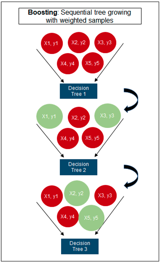
The algorithm builds upon the previous work on Decision Trees, Bagging, Random Forest, Boosting and Gradient Boosting. The benefits of using these various approaches are well know, researched, developed and proven over many years. XGBoost can be used for the typical use cases of Classification including classification, regression and ranking problems. Check out the original research paper for more details of the inner workings of the algorithm.
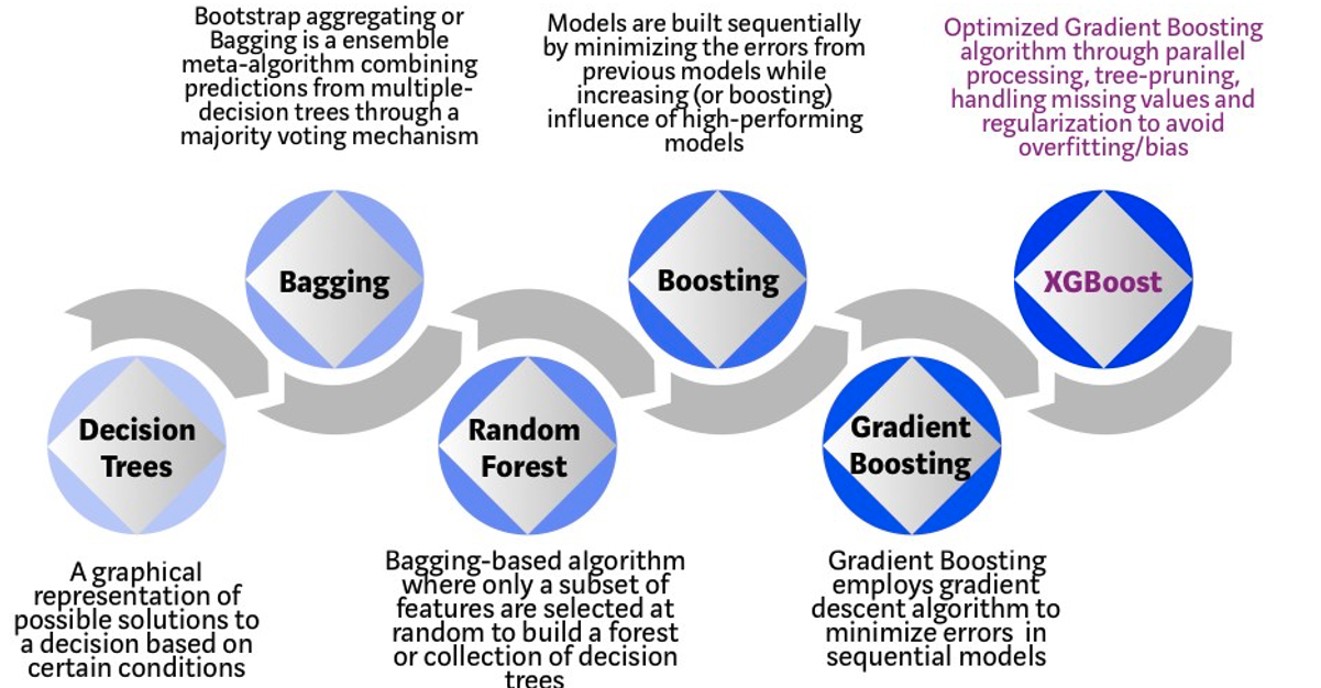
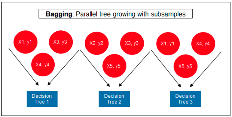
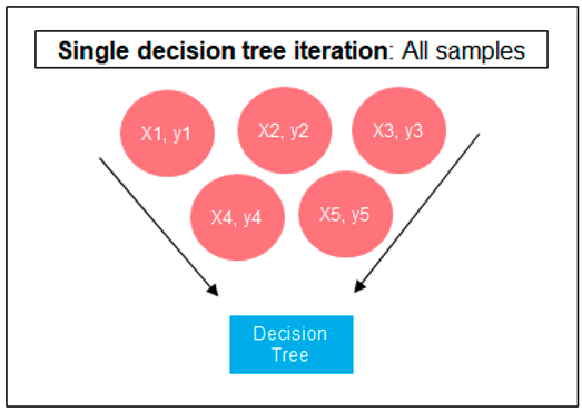
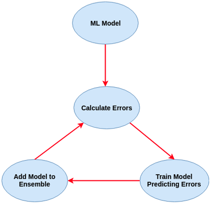 Regular machine learning models, like Decision Trees, simply train a single model using a training data set, and only this model is used for predictions. Although a Decision Tree is very simple to create (and very very quick to do so) its predictive power may not be as good as most other algorithms, despite providing model explainability. To overcome this limitation ensemble approaches can be used to create multiple Decision Trees and combines these for predictive purposes. Bagging is an approach where the predictions from multiple DT models are combined using majority voting. Building upon the bagging approach Random Forest uses different subsets of features and subsets of the training data, combining these in different ways to create a collection of DT models and presented as one model to the user. Boosting takes a more iterative approach to refining the models by building sequential models with each subsequent model is focused on minimizing the errors of the previous model. Gradient Boosting uses gradient descent algorithm to minimize errors in subsequent models. Finally with XGBoost builds upon these previous steps enabling parallel processing, tree pruning, missing data treatment, regularization and better cache, memory and hardware optimization. It’s commonly referred to as gradient boosting on steroids.
The following three images illustrates the differences between Decision Trees, Random Forest and XGBoost.
The XGBoost algorithm in Oracle 20c has over 40 different parameter settings, and with most scenarios the default settings with be fine for most scenarios. Only after creating a baseline model with the details will you look to explore making changes to these. Some of the typical settings include:
- Booster = gbtree
- #rounds for boosting = 10
- max_depth = 6
- num_parallel_tree = 1
- eval_metric = Classification error rate or RMSE for regression
As with most of the Oracle in-database machine learning algorithms, the setup and defining the parameters is really simple. Here is an example of minimum of parameter settings that needs to be defined.
BEGIN
   -- delete previous setttings
   DELETE FROM banking_xgb_settings;

   INSERT INTO BANKING_XGB_SETTINGS (setting_name, setting_value)
   VALUES (dbms_data_mining.algo_name, dbms_data_mining.algo_xgboost);

   -- For 0/1 target, choose binary:logistic as the objective.
   INSERT INTO BANKING_XGB_SETTINGS (setting_name, setting_value)
   VALUES (dbms_data_mining.xgboost_objective, 'binary:logistic’);

   commit;
END;
To create an XGBoost model run the following.


BEGIN
   DBMS_DATA_MINING.CREATE_MODEL (
      model_name          => 'BANKING_XGB_MODEL',
      mining_function     => dbms_data_mining.classification,
      data_table_name     => 'BANKING_72K',
      case_id_column_name => 'ID',
      target_column_name  => 'TARGET',
      settings_table_name => 'BANKING_XGB_SETTINGS');
END;
That’s all nice and simple, as it should be, and the new model can be called in the same manner as any of the other in-database machine learning models using functions like PREDICTION, PREDICTION_PROBABILITY, etc.
One of the interesting things I found when experimenting with XGBoost was the time it took to create the completed model. Using the default settings the following table gives the time taken, in seconds to create the model.
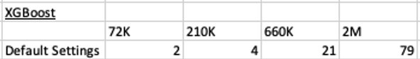
As you can see it is VERY quick even for large data sets and gives greater predictive accuracy.
MSET (Multivariate State Estimation Technique) in Oracle 20c
Updated: Changed 20c to Oracle 21c, as Oracle 20c Database never really existed 🙂
Oracle 21c Database comes with some new in-database Machine Learning algorithms.
The short name for one of these is called MSET or Multivariate State Estimation Technique. That’s the simple short name. The more complete name is Multivariate State Estimation Technique – Sequential Probability Ratio Test. That is a long name, and the reason is it consists of two algorithms. The first part looks at creating a model of the training data, and the second part looks at how new data is statistical different to the training data.
What are the use cases for this algorithm? This algorithm can be used for anomaly detection.

Anomaly Detection, using algorithms, is able identifying unexpected items or events in data that differ to the norm. It can be easy to perform some simple calculations and graphics to examine and present data to see if there are any patterns in the data set. When the data sets grow it is difficult for humans to identify anomalies and we need the help of algorithms.
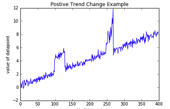
The images shown here are easy to analyze to spot the anomalies and it can be relatively easy to build some automated processing to identify these. Most of these solutions can be considered AI (Artificial Intelligence) solutions as they mimic human behaviors to identify the anomalies, and these example don’t need deep learning, neural networks or anything like that.
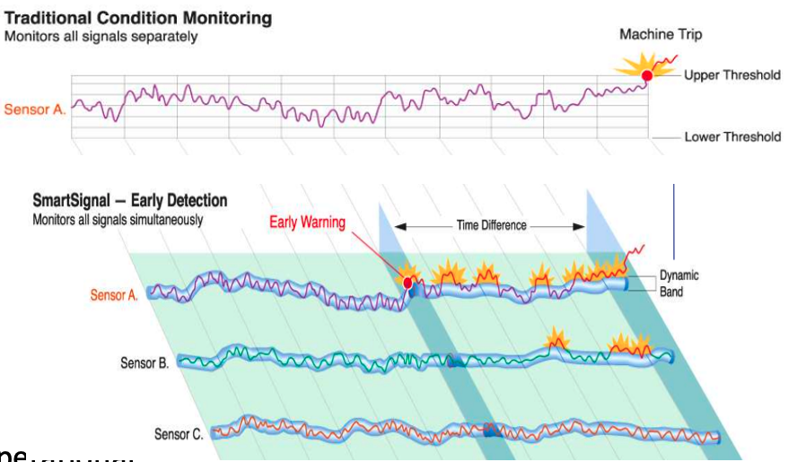
Other types of anomalies can be easily spotted in charts or graphics, such as the chart below.
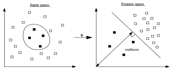 There are many different algorithms available for anomaly detection, and the Oracle Database already has an algorithm called the One-Class Support Vector Machine. This is a variant of the main Support Vector Machine (SVD) algorithm, which maps or transforms the data, using a Kernel function, into space such that the data belonging to the class values are transformed by different amounts. This creates a Hyperplane between the mapped/transformed values and hopefully gives a large margin between the mapped/transformed points. This is what makes SVD very accurate, although it does have some scaling limitations. For a One-Class SVD, a similar process is followed. The aim is for anomalous data to be mapped differently to common or non-anomalous data, as shown in the following diagram.
Getting back to the MSET algorithm. Remember it is a 2-part algorithm abbreviated to MSET. The first part is a non-linear, nonparametric anomaly detection algorithm that calibrates the expected behavior of a system based on historical data from the normal sequence of monitored signals. Using data in time series format (DATE, Value) the training data set contains data consisting of “normal” behavior of the data. The algorithm creates a model to represent this “normal”/stationary data/behavior. The second part of the algorithm compares new or live data and calculates the differences between the estimated and actual signal values (residuals). It uses Sequential Probability Ratio Test (SPRT) calculations to determine whether any of the signals have become degraded. As you can imagine the creation of the training data set is vital and may consist of many iterations before determining the optimal training data set to use.
MSET has its origins in computer hardware failures monitoring. Sun Microsystems have been were using it back in the late 1990’s-early 2000’s to monitor and detect for component failures in their servers. Since then MSET has been widely used in power generation plants, airplanes, space travel, Disney uses it for equipment failures, and in more recent times has been extensively used in IOT environments with the anomaly detection focused on signal anomalies.
How does MSET work in Oracle 21c?
An important point to note before we start is, you can use MSET on your typical business data and other data stored in the database. It isn’t just for sensor, IOT, etc data mentioned above and can be used in many different business scenarios.
The first step you need to do is to create the time series data. This can be easily done using a view, but a Very important component is the Time attribute needs to be a DATE format. Additional attributes can be numeric data and these will be used as input to the algorithm for model creation.
-- Create training data set for MSET
CREATE OR REPLACE VIEW mset_train_data
AS SELECT time_id,
          sum(quantity_sold) quantity,
          sum(amount_sold) amount
FROM (SELECT * FROM sh.sales WHERE time_id <= '30-DEC-99’)
GROUP BY time_id
ORDER BY time_id;
The example code above uses the SH schema data, and aggregates the data based on the TIME_ID attribute. This attribute is a DATE data type. The second import part of preparing and formatting the data is Ordering of the data. The ORDER BY is necessary to ensure the data is fed into or processed by the algorithm in the correct time series order.
The next step involves defining the parameters/hyper-parameters for the algorithm. All algorithms come with a set of default values, and in most cases these are suffice for your needs. In that case, you only need to define the Algorithm Name and to turn on Automatic Data Preparation. The following example illustrates this and also includes examples of setting some of the typical parameters for the algorithm.
BEGIN
  DELETE FROM mset_settings;

  -- Select MSET-SPRT as the algorithm
  INSERT  INTO mset_sh_settings (setting_name, setting_value)
  VALUES(dbms_data_mining.algo_name, dbms_data_mining.algo_mset_sprt);

  -- Turn on automatic data preparation
  INSERT INTO mset_sh_settings (setting_name, setting_value)
  VALUES(dbms_data_mining.prep_auto, dbms_data_mining.prep_auto_on);

  -- Set alert count
  INSERT INTO mset_sh_settings (setting_name, setting_value)
  VALUES(dbms_data_mining.MSET_ALERT_COUNT, 3);

  -- Set alert window
  INSERT INTO mset_sh_settings (setting_name, setting_value)
  VALUES(dbms_data_mining.MSET_ALERT_WINDOW, 5);

  -- Set alpha
  INSERT INTO mset_sh_settings (setting_name, setting_value)
  VALUES(dbms_data_mining.MSET_ALPHA_PROB, 0.1);

  COMMIT;
END;
To create the MSET model using the MST_TRAIN_DATA view created above, we can run:
BEGIN
--   DBMS_DATA_MINING.DROP_MODEL(MSET_MODEL');

   DBMS_DATA_MINING.CREATE_MODEL (
      model_name          => 'MSET_MODEL',
      mining_function     => dbms_data_mining.classification,
      data_table_name     => 'MSET_TRAIN_DATA',
      case_id_column_name => 'TIME_ID',
      target_column_name  => '',
      settings_table_name => 'MSET_SETTINGS');
END;
The SELECT statement below is an example of how to call and run the MSET model to label the data to find anomalies. The PREDICTION function will return a values of 0 (zero) or 1 (one) to indicate the predicted values. If the predicted values is 0 (zero) the MSET model has predicted the input record to be anomalous, where as a predicted values of 1 (one) indicates the value is typical. This can be used to filter out the records/data you will want to investigate in more detail.
-- display all dates with Anomalies
SELECT time_id, pred
FROM (SELECT time_id, prediction(mset_sh_model using *) over (ORDER BY time_id) pred
      FROM mset_test_data)
WHERE pred = 0;
Oracle ADW how to load new OML notebooks
Oracle Autonomous Database (ADW) has been out a while now and have had several, behind the scenes, improvements and new/additional features added.
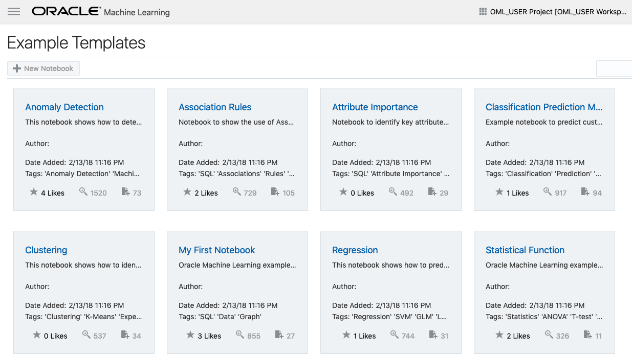
If you have used the Oracle Machine Learning (OML) component of ADW you will have seen the various sample OML Notebooks that come pre-loaded. These are easy to open, use and to try out the various OML features.

The above image shows the top part of the login screen for OML. To see the available sample notebooks click on the Examples icon. When you do, you will get the following sample OML Notebooks.
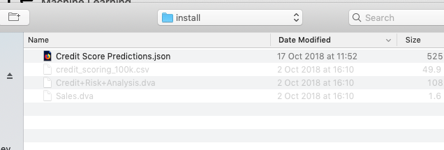
But what if you have a notebook you have used elsewhere. These can be exported in json format and loaded as a new notebook in OML.
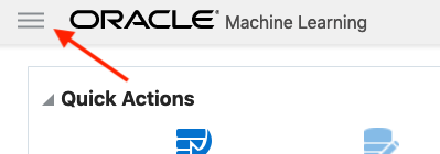
To load a new notebook into OML, select the icon (three horizontal line) on the top left hand corner of the screen. Then select Notebooks from the menu.

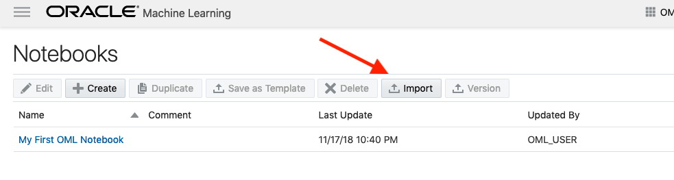
Then select the Import button located at the top of the Notebooks screen. This will open a File window, where you can select the json file from your file system.
A couple of seconds later the notebook will be available and listed along side any other notebooks you may have created.
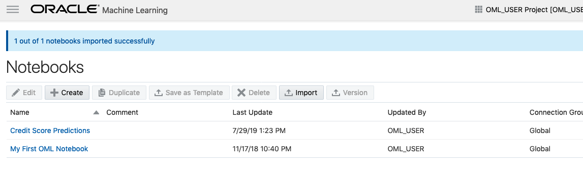
All done!
You have now imported a new notebook into OML and can now use it to process your data and perform machine learning using the in-database features.

You must be logged in to post a comment.