Vector Search

Vector Databases – Part 7 – Some simple SQL Queries

Posted on Updated on

It can be very straightforward to use Vectors using SQL. It’s just a simple SQL query, with some additional Vector related requirements. The examples given below are a collection of some simple examples. These aren’t my examples, but they come from either documentation or from other examples people have come up with. I’ve tried to include references back to the original sources for these, and if I’ve missed any or referred to the wrong people, just let me know and I’ll correct the links.

In my next post on Vector Databases, I’ll explore a slightly more complex data set. I’ll use the Wine dataset used in a previous post and Vector Search to see if I can find a suitable wine. Some years ago, I had posts and presentations on machine learning to recommend wine. Using Vector Search should give us better recommendations (hopefully)!

This first example is from the Oracle Documentation on Vector Search. This contains very simple vectors for the embedding. In my previous posts I’ve shown how to generate more complex vectors from OpenAI and Cohere.

-- In the VECTORAI user run the following

-- create demo table -- Galazies
CREATE TABLE if not exists galaxies (
 id NUMBER, 
 name VARCHAR2(50), 
 doc VARCHAR2(500), 
 embedding VECTOR);
 
-- Insert some data
INSERT INTO galaxies VALUES (1, 'M31', 'Messier 31 is a barred spiral galaxy in the Andromeda constellation which has a lot of barred spiral galaxies.', '[0,2,2,0,0]');
INSERT INTO galaxies VALUES (2, 'M33', 'Messier 33 is a spiral galaxy in the Triangulum constellation.', '[0,0,1,0,0]');
INSERT INTO galaxies VALUES (3, 'M58', 'Messier 58 is an intermediate barred spiral galaxy in the Virgo constellation.', '[1,1,1,0,0]');
INSERT INTO galaxies VALUES (4, 'M63', 'Messier 63 is a spiral galaxy in the Canes Venatici constellation.', '[0,0,1,0,0]');
INSERT INTO galaxies VALUES (5, 'M77', 'Messier 77 is a barred spiral galaxy in the Cetus constellation.', '[0,1,1,0,0]');
INSERT INTO galaxies VALUES (6, 'M91', 'Messier 91 is a barred spiral galaxy in the Coma Berenices constellation.', '[0,1,1,0,0]');
INSERT INTO galaxies VALUES (7, 'M49', 'Messier 49 is a giant elliptical galaxy in the Virgo constellation.', '[0,0,0,1,1]');
INSERT INTO galaxies VALUES (8, 'M60', 'Messier 60 is an elliptical galaxy in the Virgo constellation.', '[0,0,0,0,1]');
INSERT INTO galaxies VALUES (9, 'NGC1073', 'NGC 1073 is a barred spiral galaxy in Cetus constellation.', '[0,1,1,0,0]');
COMMIT;

-- How similar is galazy M31 to all the others
--   using VECTOR_DISTANCE to compare vectors.
--   the smaller the distance measure indicates simularity
--   Default distance measure = COSINE
SELECT g1.name AS galaxy_1,
       g2.name AS galaxy_2,
       VECTOR_DISTANCE(g2.embedding, g1.embedding) AS distance
FROM galaxies g1, 
     galaxies g2
WHERE g1.id = 1 and g2.id <> 1
ORDER BY distance ASC;

-- Euclidean Distance
SELECT g1.name AS galaxy_1,
       g2.name AS galaxy_2,
       VECTOR_DISTANCE(g2.embedding, g1.embedding, EUCLIDEAN) AS distance
FROM galaxies g1, galaxies g2
WHERE g1.id = 1 and g2.id <> 1
ORDER BY distance ASC;

-- DOT Product
SELECT g1.name AS galaxy_1,
       g2.name AS galaxy_2,
       VECTOR_DISTANCE(g2.embedding, g1.embedding, DOT) AS distance
FROM galaxies g1, galaxies g2
WHERE g1.id = 1 and g2.id <> 1
ORDER BY distance ASC;

-- Manhattan
SELECT g1.name AS galaxy_1,
       g2.name AS galaxy_2,
       VECTOR_DISTANCE(g2.embedding, g1.embedding, MANHATTAN) AS distance
FROM galaxies g1, galaxies g2
WHERE g1.id = 1 and g2.id <> 1
ORDER BY distance ASC;

-- Hamming
SELECT g1.name AS galaxy_1,
       g2.name AS galaxy_2,
       VECTOR_DISTANCE(g2.embedding, g1.embedding, HAMMING) AS distance
FROM galaxies g1, galaxies g2
WHERE g1.id = 1 and g2.id <> 1
ORDER BY distance ASC;

Again from the Oracle documentation, here is an example with a more complex vector.

------------------------------------------
-- Here is a more complex Vector example
-- From Oracle Documentation
------------------------------------------
DROP TABLE if not exists doc_queries PURGE;
CREATE TABLE doc_queries (id NUMBER, query VARCHAR2(500), embedding VECTOR);

DECLARE
  e CLOB;
BEGIN
e:= 
'[-7.73346797E-002,1.09683955E-002,4.68435362E-002,2.57333983E-002,6.95586428E-00'||
'2,-2.43412293E-002,-7.25011379E-002,6.66433945E-002,3.78751606E-002,-2.22354475E'||
'-002,3.02388351E-002,9.36625451E-002,-1.65204913E-003,3.50606232E-003,-5.4773859'||
'7E-002,-7.5879097E-002,-2.72218436E-002,7.01764375E-002,-1.32512336E-003,3.14728'||
'022E-002,-1.39147148E-001,-7.52705336E-002,2.62449421E-002,1.91645715E-002,4.055'||
'73137E-002,5.83701171E-002,-3.26474942E-002,2.0509012E-002,-3.81141738E-003,-7.1'||
'8656182E-002,-1.95893757E-002,-2.56917924E-002,-6.57705888E-002,-4.39117625E-002'||
',-6.82357177E-002,1.26592368E-001,-3.46683599E-002,1.07687116E-001,-3.96954492E-'||
'002,-9.06721968E-003,-2.4109887E-002,-1.29214963E-002,-4.82468568E-002,-3.872307'||
'76E-002,5.13443872E-002,-1.40985977E-002,-1.87066793E-002,-1.11725368E-002,9.367'||
'76772E-002,-6.39425665E-002,3.13162468E-002,8.61801133E-002,-5.5481784E-002,4.13'||
'125418E-002,2.0447813E-002,5.03717586E-002,-1.73418857E-002,3.94522659E-002,-7.2'||
'6833269E-002,3.13266069E-002,1.2377765E-002,7.64856935E-002,-3.77447419E-002,-6.'||
'41075056E-003,1.1455299E-001,1.75497644E-002,4.64923214E-003,1.89623125E-002,9.1'||
'3506597E-002,-8.22509527E-002,-1.28537193E-002,1.495138E-002,-3.22528258E-002,-4'||
'.71280375E-003,-3.15563753E-003,2.20409594E-002,7.77796134E-002,-1.927099E-002,-'||
'1.24283969E-001,4.69769612E-002,1.78121701E-002,1.67152807E-002,-3.83916795E-002'||
',-1.51029453E-002,2.10864041E-002,6.86845928E-002,-7.4719809E-002,1.17681816E-00'||
'3,3.93113159E-002,6.04066066E-002,8.55340436E-002,3.68878953E-002,2.41579115E-00'||
'2,-5.92489541E-002,-1.21883564E-002,-1.77226216E-002,-1.96259264E-002,8.51236377'||
'E-003,1.43039867E-001,2.62829307E-002,2.96348184E-002,1.92485824E-002,7.66567141'||
'E-002,-1.18600562E-001,3.01779062E-002,-5.88010997E-002,7.07774982E-002,-6.60426'||
'617E-002,6.44619241E-002,1.29240509E-002,-2.51785964E-002,2.20869959E-004,-2.514'||
'38171E-002,5.52265197E-002,8.65883753E-002,-1.83726232E-002,-8.13263431E-002,1.1'||
'6624301E-002,1.63392909E-002,-3.54643688E-002,2.05128491E-002,4.67337575E-003,1.'||
'20488718E-001,-4.89500947E-002,-3.80397178E-002,6.06209273E-003,-1.37961926E-002'||
',4.68355882E-031,3.35873142E-002,6.20040558E-002,2.13472452E-002,-1.87379227E-00'||
'3,-5.83158981E-004,-4.04266678E-002,2.40761992E-002,-1.93725452E-002,9.3763724E-'||
'002,-3.02913114E-002,7.67844869E-003,6.11112304E-002,6.02455214E-002,-6.38855845'||
'E-002,-8.03523697E-003,2.08786246E-003,-7.45898336E-002,8.74964818E-002,-5.02371'||
'937E-002,-4.99385223E-003,3.37120108E-002,8.99377018E-002,1.09540671E-001,5.8501'||
'102E-002,1.71627291E-002,-3.26152593E-002,8.36912021E-002,5.05600758E-002,-9.737'||
'63615E-002,-1.40264994E-002,-2.07926836E-002,-4.20163684E-002,-5.97197041E-002,1'||
'.32461395E-002,2.26361351E-003,8.1473738E-002,-4.29272018E-002,-3.86809185E-002,'||
'-8.24682564E-002,-3.89646105E-002,1.9992901E-002,2.07321253E-002,-1.74706057E-00'||
'2,4.50415723E-003,4.43851873E-002,-9.86309871E-002,-7.68082142E-002,-4.53814305E'||
'-003,-8.90906602E-002,-4.54972908E-002,-5.71065396E-002,2.10020249E-003,1.224947'||
'07E-002,-6.70659095E-002,-6.52298108E-002,3.92126441E-002,4.33384106E-002,4.3899'||
'6181E-002,5.78813367E-002,2.95345876E-002,4.68395352E-002,9.15119275E-002,-9.629'||
'58392E-003,-5.96637605E-003,1.58674959E-002,-6.74034096E-003,-6.00510836E-002,2.'||
'67188111E-003,-1.10706768E-003,-6.34015873E-002,-4.80389707E-002,6.84534572E-003'||
',-1.1547043E-002,-3.44865513E-003,1.18979132E-002,-4.31232266E-002,-5.9022788E-0'||
'02,4.87607308E-002,3.95954074E-003,-7.95252472E-002,-1.82770658E-002,1.18264249E'||
'-002,-3.79164703E-002,3.87993976E-002,1.09805465E-002,2.29136664E-002,-7.2278082'||
'4E-002,-5.31538352E-002,6.38669729E-002,-2.47980515E-003,-9.6999377E-002,-3.7566'||
'7699E-002,4.06541862E-002,-1.69874367E-003,5.58868013E-002,-1.80723771E-033,-6.6'||
'5985467E-003,-4.45010923E-002,1.77929532E-002,-4.8369132E-002,-1.49722975E-002,-'||
'3.97582203E-002,-7.05247298E-002,3.89178023E-002,-8.26886389E-003,-3.91006246E-0'||
'02,-7.02963024E-002,-3.91333885E-002,1.76661201E-002,-5.09723537E-002,2.37749107'||
'E-002,-1.83419678E-002,-1.2693027E-002,-1.14232123E-001,-6.68751821E-002,7.52167'||
'869E-003,-9.94713791E-003,6.03599809E-002,6.61353692E-002,3.70595567E-002,-2.019'||
'52495E-002,-2.40410417E-002,-3.36526595E-002,6.20064288E-002,5.50279953E-002,-2.'||
'68641673E-002,4.35859226E-002,-4.57317568E-002,2.76936609E-002,7.88119733E-002,-'||
'4.78852056E-002,1.08523415E-002,-6.43479973E-002,2.0192951E-002,-2.09538229E-002'||
',-2.2202393E-002,-1.0728148E-003,-3.09607089E-002,-1.67067181E-002,-6.03572279E-'||
'002,-1.58187654E-002,3.45828459E-002,-3.45360823E-002,-4.4002533E-003,1.77463517'||
'E-002,6.68234832E-004,6.14458732E-002,-5.07084019E-002,-1.21073434E-002,4.195981'||
'85E-002,3.69152687E-002,1.09461844E-002,1.83413982E-001,-3.89185362E-002,-5.1846'||
'0497E-002,-8.71620141E-003,-1.17692262E-001,4.04785499E-002,1.07505821E-001,1.41'||
'624091E-002,-2.57720836E-002,2.6652012E-002,-4.50568087E-002,-3.34110335E-002,-1'||
'.11387551E-001,-1.29796984E-003,-6.51671961E-002,5.36890551E-002,1.0702607E-001,'||
'-2.34011523E-002,3.97406481E-002,-1.01149324E-002,-9.95831117E-002,-4.40197848E-'||
'002,6.88989647E-003,4.85475454E-003,-3.94048765E-002,-3.6099229E-002,-5.4075513E'||
'-002,8.58292207E-002,1.0697281E-002,-4.70785573E-002,-2.96272673E-002,-9.4919120'||
'9E-003,1.57316476E-002,-5.4926388E-002,6.49022609E-002,2.55531631E-002,-1.839057'||
'17E-002,4.06873561E-002,4.74951901E-002,-1.22502812E-033,-4.6441108E-002,3.74079'||
'868E-002,9.14599106E-004,6.09740615E-002,-7.67391697E-002,-6.32521287E-002,-2.17'||
'353106E-002,2.45231949E-003,1.50869079E-002,-4.96984981E-002,-3.40828523E-002,8.'||
'09691194E-003,3.31339166E-002,5.41345142E-002,-1.16213948E-001,-2.49572527E-002,'||
'5.00682592E-002,5.90037219E-002,-2.89178211E-002,8.01460445E-003,-3.41945067E-00'||
'2,-8.60121697E-002,-6.20261126E-004,2.26721354E-002,1.28968194E-001,2.87655368E-'||
'002,-2.20255274E-002,2.7228903E-002,-1.12029864E-002,-3.20301466E-002,4.98079099'||
'E-002,2.89051589E-002,2.413591E-002,3.64605561E-002,6.26017479E-003,6.54632896E-'||
'002,1.11282602E-001,-3.60428065E-004,1.95987038E-002,6.16615731E-003,5.93593046E'||
'-002,1.50377362E-003,2.95319762E-002,2.56325547E-002,-1.72190219E-002,-6.5816819'||
'7E-002,-4.08149995E-002,2.7983617E-002,-6.80195764E-002,-3.52494679E-002,-2.9840'||
'0577E-002,-3.04043181E-002,-1.9352382E-002,5.49411364E-002,8.74160081E-002,5.614'||
'25127E-002,-5.60747795E-002,-3.43311466E-002,9.83581021E-002,2.01142877E-002,1.3'||
'193069E-002,-3.22583504E-002,8.54402035E-002,-2.20514946E-002]';

INSERT INTO doc_queries VALUES (13, 'different methods of backup and recovery', e);
COMMIT;
END;
/

The next example is a really nice one, so check out the link to the original post. They give some charts which plot the vectors. You can use these to easily visualize the data points and why we get our answers to the queries.

-----------------------
-- Another example
-- taken from https://medium.com/@ludan.aguirre/oracle-23ai-vector-search-its-all-about-semantics-f9224ac6d4bb
-----------------------

CREATE TABLE if not exists PARKING_LOT (
 VEHICLE VARCHAR2(10),
 LOCATION VECTOR
);

INSERT INTO PARKING_LOT VALUES('CAR1','[7,4]');
INSERT INTO PARKING_LOT VALUES('CAR2','[3,5]');
INSERT INTO PARKING_LOT VALUES('CAR3','[6,2]');
INSERT INTO PARKING_LOT VALUES('TRUCK1','[10,7]');
INSERT INTO PARKING_LOT VALUES('TRUCK2','[4,7]');
INSERT INTO PARKING_LOT VALUES('TRUCK3','[2,3]');
INSERT INTO PARKING_LOT VALUES('TRUCK4','[5,6]');
INSERT INTO PARKING_LOT VALUES('BIKE1','[4,1]');
INSERT INTO PARKING_LOT VALUES('BIKE2','[6,5]');
INSERT INTO PARKING_LOT VALUES('BIKE3','[2,6]');
INSERT INTO PARKING_LOT VALUES('BIKE4','[5,8]');
INSERT INTO PARKING_LOT VALUES('SUV1','[8,2]');
INSERT INTO PARKING_LOT VALUES('SUV2','[9,5]');
INSERT INTO PARKING_LOT VALUES('SUV3','[1,2]');
INSERT INTO PARKING_LOT VALUES('SUV4','[5,4]');

select
v1.vehicle as vehicle_1,
v2.vehicle as vehicle_2,
VECTOR_DISTANCE(v1.location,v2.location,EUCLIDEAN) as distance
from parking_lot v1, parking_lot v2
where v1.vehicle='CAR1'
order by distance asc
FETCH FIRST 6 ROWS ONLY;


select
v1.vehicle as vehicle_1,
v2.vehicle as vehicle_2,
VECTOR_DISTANCE(v1.location,v2.location,EUCLIDEAN) as distance
from parking_lot v1, parking_lot v2
where v1.vehicle='TRUCK4'
order by distance asc
FETCH FIRST 6 ROWS ONLY;

I’ll have another post on using Vector Search to explore and make Wine recommendations based on personalized tastes etc.

Vector Databases – Part 5 – SQL function to call External Embedding model

Posted on Updated on

There are several ways to create Vector embedding. In previous posts, I’ve provided some examples (see links below). These examples were externally created and then loaded into the database.

But what if we want to do this internally in the database? We can use SQL and create a new vector embedding every time we insert or update a record.

The following examples are based on using the Oracle 23.5ai Virtual Machine. These examples illustrate using a Cohere Embedding model. At time of writing this post using OpenAI generates an error. In theory it should work and might work with subsequent database releases. All you need to do is include your OpenAI key and model to use.

Step-1 : DBA tasks

Log into the SYSTEM schema for the 23.5ai Database on the VM. You can do this using SQLcl, VS Code, SQL Developer or whatever is your preferred tool. I’m assuming you have a schema in the DB you want to use. In my example, this schema is called VECTORAI. Run the following:

BEGIN
  DBMS_NETWORK_ACL_ADMIN.APPEND_HOST_ACE(
    host => '*',
    ace => xs$ace_type(privilege_list => xs$name_list('connect'),
                       principal_name => 'vectorai',
                       principal_type => xs_acl.ptype_db));
END;


grant create credential to vectorai;

This code will open the database to the outside world to all available site, host => ‘*’. This is perhaps a little dangerous and should be restricted to only the site you want access to. Then grant an additional privilege to VECTORAI which allows it to create credentials. We’ll use this in the next step.

Steps 2 – In Developer Schema (vectorai)

Next, log into your developer schema. In this example, I’m using a schema called VECTORAI.

Step 3 – Create a Credential

Create a credential which points to your API Key. In this example, I’m connecting to my Cohere API key.

DECLARE
  jo json_object_t;
BEGIN
  jo := json_object_t();
  jo.put('access_token', '...');
  dbms_vector.create_credential(
    credential_name   => 'CRED_COHERE',
    params            => json(jo.to_string));
END;

Enter your access token in the above, replacing the ‘…’

Step 4 – Test calling the API to return a Vector

Use the following code to test calling an Embedding Model passing some text to parse.

declare
  input clob;
  params clob;
  output clob;
  v VECTOR;
begin
--  input := 'hello';
  input := 'Aromas include tropical fruit, broom, brimstone and dried herb. The palate isnt overly expressive, offering unripened apple, citrus and dried sage alongside brisk acidity.';

  params := '
{
  "provider": "cohere",
  "credential_name": "CRED_COHERE",
  "url": "https://api.cohere.ai/v1/embed",
  "model": "embed-english-v2.0"
}';

  v := dbms_vector.utl_to_embedding(input, json(params));
  output := to_clob(v);
  dbms_output.put_line('VECTOR');
  dbms_output.put_line('--------------------');
  dbms_output.put_line(dbms_lob.substr(output,1000)||'...');
exception
  when OTHERS THEN
    DBMS_OUTPUT.PUT_LINE (SQLERRM);
    DBMS_OUTPUT.PUT_LINE (SQLCODE);
end;

This should generate something like the following with the Vector values.

VECTOR

--------------------

[-1.33886719E+000,-3.61816406E-001,7.50488281E-001,5.11230469E-001,-3.63037109E-001,1.5222168E-001,1.50390625E+000,-1.81674957E-004,-4.65087891E-002,-7.48535156E-001,-8.62426758E-002,-1.24414062E+000,-1.02148438E+000,1.19433594E+000,1.41503906E+000,-7.02148438E-001,-1.66015625E+000,2.39990234E-001,8.68652344E-001,1.90917969E-001,-3.17871094E-001,-7.08007812E-001,-1.29882812E+000,-5.63476562E-001,-5.65429688E-001,-7.60498047E-002,-1.40820312E+000,1.01367188E+000,-6.45996094E-001,-1.38574219E+000,2.31054688E+000,-1.21191406E+000,6.65893555E-002,1.02148438E+000,-8.16040039E-002,-5.17578125E-001,1.61035156E+000,1.23242188E+000,1.76879883E-001,-5.71777344E-001,1.45214844E+000,1.30957031E+000,5.30395508E-002,-1.38476562E+000,1.00976562E+000,1.36425781E+000,8.8671875E-001,1.578125E+000,7.93457031E-001,1.03027344E+000,1.33007812E+000,1.08300781E+000,-4.21875E-001,-1.23535156E-001,1.31933594E+000,-1.21191406E+000,4.49462891E-001,-1.06640625E+000,5.26367188E-001,-1.95214844E+000,1.58105469E+000,...

The Vector displayed above has been truncated, as the vector contains 4096 dimensions. If you’d prefer to work with a smaller number of dimensions you could use the ’embed-english-light-v2.0′ embedding model.

An alternative way to test this is using SQLcl and run the following:

var params clob;
exec :params := '{"provider": "cohere", "credential_name": "CRED_COHERE", "url": "https://api.cohere.ai/v1/embed", "model": "embed-english-v2.0"}';
select dbms_vector.utl_to_embedding('hello', json(:params)) from dual;

In this example, the text to be converted into a vector is ‘hello’

Step 5 – Create an Insert/Update Trigger on table.

Let’s create a test table.

create table vec_test (col1 number, col2 varchar(200), col3 vector);

Using the code from the previous step, we can create an insert/update trigger.

create or replace trigger vec_test_trig
   before insert or update on vec_test
for each row
declare
   params clob;
   v  vector;
begin
   params := '
{
  "provider": "cohere",
  "credential_name": "CRED_COHERE",
  "url": "https://api.cohere.ai/v1/embed",
  "model": "embed-english-v2.0"
}';

  v := dbms_vector.utl_to_embedding(:new.col2, json(params));
  :new.col3 := v;
end;

We can easily test this trigger and the inserting/updating of the vector embedding using the following.

insert into vec_test values (1, 'Aromas include tropical fruit, broom, brimstone and dried herb', null);

select * from vec_test;

update VEC_TEST
set col2 = 'Wonderful aromas, lots of fruit, dark cherry and oak'
where col1 = 1;

select * from vec_test;

When you inspect the table after the insert statement, you’ll see the vector has been added. Then after the update statement, you’ll be able to see we have a new vector for the record.

Vector Databases – Part 4 – Vector Indexes

Posted on Updated on

In this post on Vector Databases, I’ll explore some of the commonly used indexing techniques available in Databases. I’ll also explore the Vector Indexes available in Oracle 23c. Be sure to check that section towards the end of the post, where I’ll also include links to other articles in this series.

As with most data in a Databases, indexes are used for fast access to data. They create an organised structure (typically B+ tree) for storing the location of certain values within a table. When searching for data, if an index exists on that data, the index will be used for matching and the location of the records is used to quickly retrieve the data.

Similarly, for Vector searches, we need some way to search through thousands or millions of vectors to find those that best match our search criteria (vector search). For vector search, there are many more calculations to perform. We want to avoid a MxN search space.

Given the nature of Vectors and the the type of search performed on these, databases need to have different types of indexes. Common Vector Index types include Hash-base, Tree-based, Graph-base and Inverted-file. Let’s have a look at each of these.

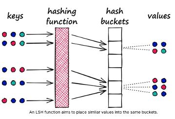
Hash-based Vector Indexes

Locality-Sensitive Hashing (LSH) uses hash functions to bucket similar vectors into a hash table. The query vectors are also hashed using the same hash function and it is compared with the other vectors already present in the table. This method is much faster than doing an exhaustive search across the entire dataset because there are fewer vectors in each hash table than in the whole vector space. While this technique is quite fast, the downside is that it is not very accurate. LSH is an approximate method, so a better hash function will result in a better approximation, but the result will not be the exact answer.

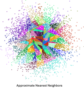
Tree-based Vector Indexes

Tree-based indexing allows for fast searches by using a data structure such as a binary tree. The tree gets created in a way that similar vectors are grouped in the same subtree. Approximate Nearest Neighbour (ANN) uses a forest of binary trees to perform approximate nearest neighbors search. ANN performs well with high-dimension data where doing an exact nearest neighbors search can be expensive. The downside of using this method is that it can take a significant amount of time to build the index. Whenever a new data point is received, the indices cannot be restructured on the fly. The entire index has to be rebuilt from scratch.

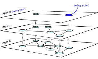
Graph-based Vector Indexes

Similar to tree-based indexing, graph-based indexing groups similar data points by connecting them with an edge. Graph-based indexing is useful when trying to search for vectors in a high-dimensional space. Hierarchical Navigable Small Worlds (HNSW) creates a layered graph with the topmost layer containing the fewest points and the bottom layer containing the most points. When an input query comes in, the topmost layer is searched via ANN. The graph is traversed downward layer by layer. At each layer, the ANN algorithm is run to find the closest point to the input query. Once the bottom layer is hit, the nearest point to the input query is returned. Graph-based indexing is very efficient because it allows one to search through a high-dimensional space by narrowing down the location at each layer. However, re-indexing can be challenging because the entire graph may need to be recreated

Inverted-FIle Vector Indexes

IVF (InVerted File) narrows the search space by partitioning the dataset and creating a centroid(random point) for each partition. The centroids get updated via the K-Means algorithm. Once the index is populated, the ANN algorithm finds the nearest centroid to the input query and only searches through that partition. Although IVF is efficient at searching for similar points once the index is created, the process of creating the partitions and centroids can be quite slow.

Oracle 23ai comes with two main types of indexes for Vectors. These are:

In-Memory – Neighbor Graph Vector Index

Hierarchical Navigable Small World (HNSW) is the only type of In-Memory Neighbor Graph vector index supported. With Navigable Small World (NSW), the idea is to build a proximity graph where each vector in the graph connects to several others based on three characteristics:

  • The distance between vectors
  • The maximum number of closest vector candidates considered at each step of the search during insertion (EFCONSTRUCTION)
  • Within the maximum number of connections (NEIGHBORS) permitted per vector

Navigable Small World (NSW) graph traversal for vector search begins with a predefined entry point in the graph, accessing a cluster of closely related vectors. The search algorithm employs two key lists:

  • Candidates, a dynamically updated list of vectors that we encounter while traversing the graph,
  • and Results, which contains the vectors closest to the query vector found thus far.

As the search progresses, the algorithm navigates through the graph, continually refining the Candidates by exploring and evaluating vectors that might be closer than those in the Results. The process concludes once there are no vectors in the Candidates closer than the farthest in the Results, indicating

Neighbor Partition Vector Index

Inverted File Flat (IVF) index is the only type of Neighbor Partition vector index supported.

Inverted File Flat Index (IVF Flat or simply IVF) is a partitioned-based index which balance high search quality with reasonable speed.

The IVF index is a technique designed to enhance search efficiency by narrowing the search area through the use of neighbor partitions or clusters.

Here is an example of creating such an index in Oracle 23ai.

CREATE VECTOR INDEX galaxies_ivf_idx ON galaxies (embedding) 
ORGANIZATION NEIGHBOR 
PARTITIONS DISTANCE COSINE 
WITH TARGET ACCURACY 95;

Check out my other posts in this series on Vector Databases.

Vector Databases – Part 3 – Vector Search

Posted on Updated on

Searching semantic similarity in a data set is now equivalent to searching for nearest neighbors in a vector space instead of using traditional keyword searches using query predicates. The distance between “dog” and “wolf” in this vector space is shorter than the distance between “dog” and “kitten”. A “dog” is more similar to a “wolf” than it is to a “kitten”.

Vector data tends to be unevenly distributed and clustered into groups that are semantically related. Doing a similarity search based on a given query vector is equivalent to retrieving the K-nearest vectors to your query vector in your vector space.

Typically, you want to find an ordered list of vectors by ranking them, where the first row in the list is the closest or most similar vector to the query vector, the second row in the list is the second closest vector to the query vector, and so on. When doing a similarity search, the relative order of distances is what really matters rather than the actual distance.

Semantic search where the initial vector is the word “Puppy” and you want to identify the four closest words. Similarity searches tend to get data from one or more clusters depending on the value of the query vector, distance and the fetch size. Approximate searches using vector indexes can limit the searches to specific clusters, whereas exact searches visit vectors across all clusters.

Measuring distances in a vector space is the core of identifying the most relevant results for a given query vector. That process is very different from the well-known keyword filtering in the relational database world, which is very quick, simple and very very efficient. Vector distance functions involve more complicated computations.

There are several ways you can calculate distances to determine how similar, or dissimilar, two vectors are. Each distance metric is computed using different mathematical formulas. The time taken to calculate the distance between two vectors depends on many factors, including the distance metric used as well as the format of the vectors themselves, such as the number of vector dimensions and the vector dimension formats.

Generally, it’s best to match the distance metric you use to the one that was used to train the vector embedding model that generated the vectors. Common Distance metric functions include:

  • Euclidean Distance
  • Euclidean Distance Squared
  • Cosine Similarity   [most commonly used]
  • Dot Product Similarity
  • Manhattan Distance Hamming Similarity
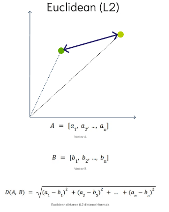
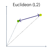
Euclidean Distance

This is a measure of the straight line distance between two points in the vector space. It ranges from 0 to infinity, where 0 represents identical vectors, and larger values represent increasingly dissimilar vectors. This is calculated using the Pythagorean theorem applied to the vector’s coordinates.

This metric is sensitive to both the vector’s size and it’s direction.

Euclidean Distance Squared

This is very similar to Euclidean Distance. When ordering is more important than the distance values themselves, the Squared Euclidean distance is very useful as it is faster to calculate than the Euclidean distance (avoiding the square-root calculation)
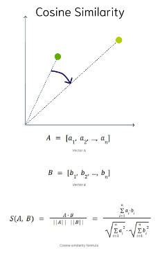
Cosine Similarity

This is the most commonly used distance measure. The cosine of the angle between two vectors – the larger the cosine, the closer the vectors. The smaller the angle, the bigger is its cosine. Cosine similarity measures the similarity in the direction or angle of the vectors, ignoring differences in their size (also called magnitude). The smaller the angle, the more similar are the two vectors. It ranges from -1 to 1, where 1 represents identical vectors, 0 represents orthogonal vectors, and -1 represents vectors that are diametrically opposed

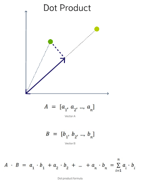
DOT Product Similarity

DOT product similarity of two vectors can be viewed as multiplying the size of each vector by the cosine of their angle. The larger the dot product, the closer the vectors. You project one vector on the other and multiply the resulting vector sizes. Larger DOT product values imply that the vectors are more similar, while smaller values imply that they are less similar. It ranges from -∞ to ∞, where a positive value represents vectors that point in the same direction, 0 represents orthogonal vectors, and a negative value represents vectors that point in opposite directions
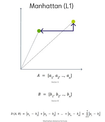
Manhattan Distance

This is calculated by summing the distance between the dimensions of the two vectors that you want to compare.

Imagine yourself in the streets of Manhattan trying to go from point A to point B. A straight line is not possible.
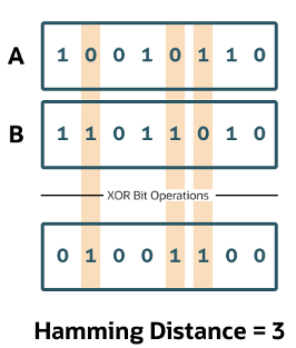
Hamming Similarity

This is the distance between two vectors represented by the number of dimensions where they differ. When using binary vectors, the Hamming distance between two vectors is the number of bits you must change to change one vector into the other. To compute the Hamming distance between two vectors, you need to compare the position of each bit in the sequence.

Check out my other posts in this series on Vector Databases.