
PL/SQL
SelectAI – the APEX version
I’ve written a few blog posts about the new Select AI feature on the Oracle Database. In this post, I’ll explore how to use this within APEX, because you have to do things in a different way.
The previous posts on Select AI are:
- SelectAI – the beginning of a journey
- SelectAI – Doing something useful
- SelectAI – Can metadata help
- SelectAI – the APEX version
We have seen in my previous posts how the PL/SQL package called DBMS_CLOUD_AI was used to create a profile. This profile provided details of what provided to use (Cohere or OpenAI in my examples), and what metadata (schemas, tables, etc) to send to the LLM. When you look at the DBMS_CLOUD_AI PL/SQL package it only contains seven functions (at time of writing this post). Most of these functions are for managing the profile, such as creating, deleting, enabling, disabling and setting the profile attributes. But there is one other important function called GENERATE. This function can be used to send your request to the LLM.
Why is the DBMS_CLOUD_AI.GENERATE function needed? We have seen in my previous posts using Select AI using common SQL tools such as SQL Developer, SQLcl and SQL Developer extension for VSCode. When using these tools we need to enable the SQL session to use Select AI by setting the profile. When using APEX or creating your own PL/SQL functions, etc. You’ll still need to set the profile, using
EXEC DBMS_CLOUD_AI.set_profile('OPEN_AI');We can now use the DBMS_CLOUD_AI.GENERATE function to run our equivalent Select AI queries. We can use this to run most of the options for Select AI including showsql, narrate and chat. It’s important to note here that runsql is not supported. This was the default action when using Select AI. Instead, you obtain the necessary SQL using showsql, and you can then execute the returned SQL yourself in your PL/SQL code.
Here are a few examples from my previous posts:
SELECT DBMS_CLOUD_AI.GENERATE(prompt       => 'what customer is the largest by sales',
                              profile_name => 'OPEN_AI',
                              action       => 'showsql')
FROM dual;

SELECT DBMS_CLOUD_AI.GENERATE(prompt       => 'how many customers in San Francisco are married',
                              profile_name => 'OPEN_AI',
                              action       => 'narrate')
FROM dual;

SELECT DBMS_CLOUD_AI.GENERATE(prompt       => 'who is the president of ireland',
                              profile_name => 'OPEN_AI',
                              action       => 'chat')
FROM dual;
If using Oracle 23c or higher you no longer need to include the FROM DUAL;
Time Series Forecasting in Oracle – Part 2
This is the second part about time-series data modeling using Oracle. Check out the first part here.
In this post I will take a time-series data set and using the in-database time-series functions model the data, that in turn can be used for predicting future values and trends.
The data set used in these examples is the Rossmann Store Sales data set. It is available on Kaggle and was used in one of their competitions.
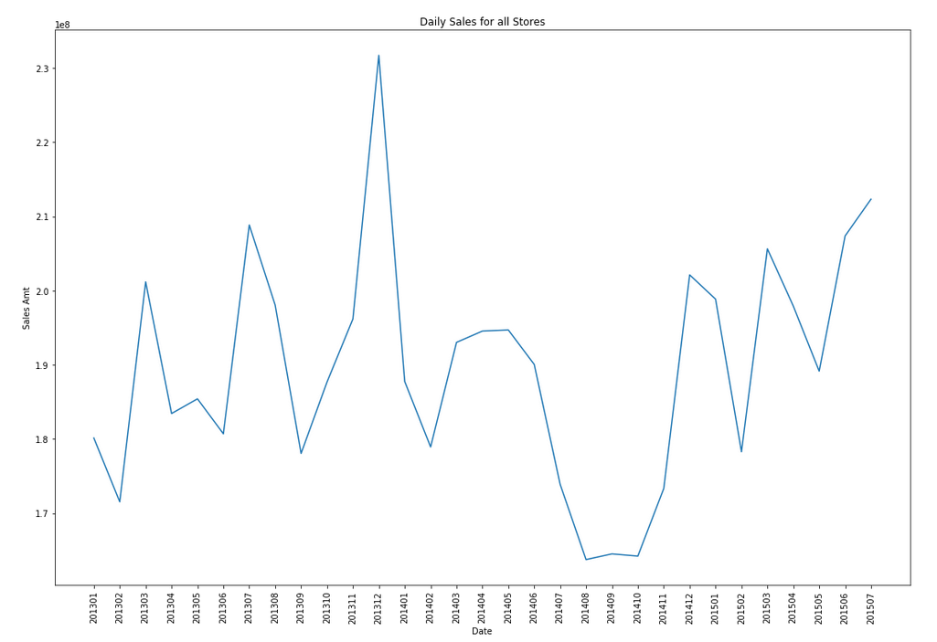
Let’s start by aggregating the data to monthly level. We get.
Data Set-up
Although not strictly necessary, but it can be useful to create a subset of your time-series data to only contain the time related attribute and the attribute containing the data to model. When working with time-series data, the exponential smoothing function expects the time attribute to be of DATE data type. In most cases it does. When it is a DATE, the function will know how to process this and all you need to do is to tell the function the interval.
A view is created to contain the monthly aggregated data.
-- Create input time series
create or replace view demo_ts_data as
select to_date(to_char(sales_date, 'MON-RRRR'),'MON-RRRR') sales_date,
sum(sales_amt) sales_amt
from demo_time_series
group by to_char(sales_date, 'MON-RRRR')
order by 1 asc;
Next a table is needed to contain the various settings for the exponential smoothing function.
CREATE TABLE demo_ts_settings(setting_name VARCHAR2(30),
                              setting_value VARCHAR2(128));
Some care is needed with selecting the parameters and their settings as not all combinations can be used.
Example 1 – Holt-Winters
The first example is to create a Holt-Winters time-series model for hour data set. For this we need to set the parameter to include defining the algorithm name, the specific time-series model to use (exsm_holt), the type/size of interval (monthly) and the number of predictions to make into the future, pass the last data point.
BEGIN
   -- delete previous setttings
   delete from demo_ts_settings;

   -- set ESM as the algorithm
   insert into demo_ts_settings
      values (dbms_data_mining.algo_name,
              dbms_data_mining.algo_exponential_smoothing);

   -- set ESM model to be Holt-Winters
   insert into demo_ts_settings
      values (dbms_data_mining.exsm_model,
              dbms_data_mining.exsm_holt);

   -- set interval to be month
   insert into demo_ts_settings
      values (dbms_data_mining.exsm_interval,
              dbms_data_mining.exsm_interval_month);

   -- set prediction to 4 steps ahead
   insert into demo_ts_settings
      values (dbms_data_mining.exsm_prediction_step,
              '4');

   commit;
END;
Now we can call the function, generate the model and produce the predicted values.
BEGIN
   -- delete the previous model with the same name
   BEGIN
      dbms_data_mining.drop_model('DEMO_TS_MODEL');
   EXCEPTION
      WHEN others THEN null;
   END;

   dbms_data_mining.create_model(model_name => 'DEMO_TS_MODEL',
                                 mining_function => 'TIME_SERIES',
                                 data_table_name => 'DEMO_TS_DATA',
                                 case_id_column_name => 'SALES_DATE',
                                 target_column_name => 'SALES_AMT',
                                 settings_table_name => 'DEMO_TS_SETTINGS');
END;
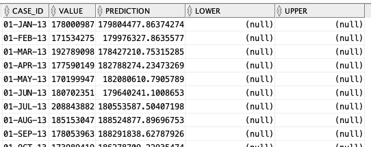
When the model is created a number of data dictionary views are populated with model details and some addition views are created specific to the model. One such view commences with DM$VP. Views commencing with this contain the predicted values for our time-series model. You need to append the name of the model created, in our example DEMO_TS_MODEL.
-- get predictions
select case_id, value, prediction, lower, upper
from   DM$VPDEMO_TS_MODEL
order by case_id;
When we plot this data we get.
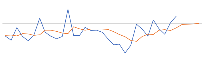
The blue line contains the original data values and the red line contains the predicted values. The predictions are very similar to those produced using Holt-Winters in Python.
Example 2 – Holt-Winters including Seasonality
The previous example didn’t really include seasonality into the model and predictions. In this example we introduce seasonality to allow the model to pick up any trends in the data based on a defined period.
For this example we will change the model name to HW_ADDSEA, and the season size to 5 units. A data set with a longer time period would illustrate the different seasons better but this gives you an idea.
BEGIN
   -- delete previous setttings
   delete from demo_ts_settings;

   -- select ESM as the algorithm
   insert into demo_ts_settings
   values (dbms_data_mining.algo_name,
           dbms_data_mining.algo_exponential_smoothing);

   -- set ESM model to be Holt-Winters Seasonal Adjusted
   insert into demo_ts_settings
   values (dbms_data_mining.exsm_model,
           dbms_data_mining.exsm_HW_ADDSEA);

   -- set interval to be month
   insert into demo_ts_settings
   values (dbms_data_mining.exsm_interval,
   dbms_data_mining.exsm_interval_month);

  -- set prediction to 4 steps ahead
  insert into demo_ts_settings
  values (dbms_data_mining.exsm_prediction_step,
          '4');

   -- set seasonal cycle to be 5 quarters
   insert into demo_ts_settings
   values (dbms_data_mining.exsm_seasonality,
           '5');

commit;
END;
We need to re-run the creation of the model and produce the predicted values. This code is unchanged from the previous example.
BEGIN
   -- delete the previous model with the same name
   BEGIN
      dbms_data_mining.drop_model('DEMO_TS_MODEL');
   EXCEPTION
      WHEN others THEN null;
   END;

   dbms_data_mining.create_model(model_name => 'DEMO_TS_MODEL',
                                 mining_function => 'TIME_SERIES',
                                 data_table_name => 'DEMO_TS_DATA',
                                 case_id_column_name => 'SALES_DATE',
                                 target_column_name => 'SALES_AMT',
                                 settings_table_name => 'DEMO_TS_SETTINGS');
END;
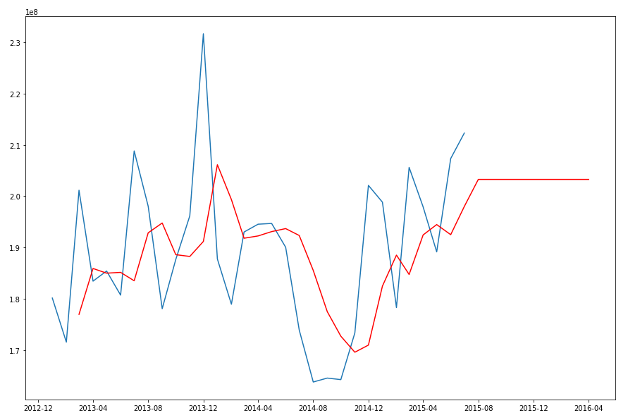
When we re-query the DM$VPDEMO_TS_MODEL we get the new values. When plotted we get.
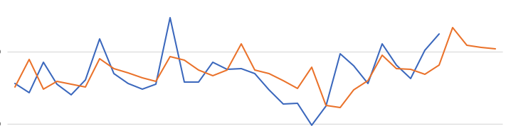
The blue line contains the original data values and the red line contains the predicted values.
Comparing this chart to the chart from the first example we can see there are some important differences between them. These differences are particularly evident in the second half of the chart, on the right hand side. We get to see there is a clearer dip in the predicted data. This mirrors the real data values better. We also see better predictions as the time line moves to the end.
When performing time-series analysis you really need to spend some time exploring the data, to understand what is happening, visualizing the data, seeing if you can identify any patterns, before moving onto using the different models. Similarly you will need to explore the various time-series models available and the parameters, to see what works for your data and follow the patterns in your data. There is no magic solution in this case.
Explicit Semantic Analysis setup using SQL and PL/SQL
In my previous blog post I introduced the new Explicit Semantic Analysis (ESA) algorithm and gave an example of how you can build an ESA model and use it. Check out this link for that blog post.
In this blog post I will show you how you can manually create an ESA model. The reason that I’m showing you this way is that the workflow (in ODMr and it’s scheduler) may not be for everyone. You may want to automate the creation or recreation of the ESA model from time to time based on certain business requirements.
In my previous blog post I showed how you can setup a training data set. This comes with ODMr 4.2 but you may need to expand this data set or to use an alternative data set that is more in keeping with your domain.
Setup the ODM Settings table
As with all ODM algorithms we need to create a settings table. This settings table allows us to store the various parameters and their values, that will be used by the algorithm.
-- Create the settings table
CREATE TABLE ESA_settings (
    setting_name VARCHAR2(30),
    setting_value VARCHAR2(30));

-- Populate the settings table
-- Specify ESA. By default, Naive Bayes is used for classification.
-- Specify ADP. By default, ADP is not used. Need to turn this on.
BEGIN
    INSERT INTO ESA_settings (setting_name, setting_value)
    VALUES (dbms_data_mining.algo_name,
           dbms_data_mining.algo_explicit_semantic_analys);

    INSERT INTO ESA_settings (setting_name, setting_value)
    VALUES (dbms_data_mining.prep_auto,dbms_data_mining.prep_auto_on);

    INSERT INTO ESA_settings (setting_name, setting_value)
    VALUES (odms_sampling,odms_sampling_disable);

    commit;
END;
These are the minimum number of parameter setting needed to run the ESA algorithm. The other ESA algorithm setting include:

Setup the Oracle Text Policy
You also need to setup an Oracle Text Policy and a lexer for the Stopwords.
DECLARE
   v_policy_name  varchar2(30);
   v_lexer_name   varchar2(3)
BEGIN
    v_policy_name  := 'ESA_TEXT_POLICY';
    v_lexer_name   := 'ESA_LEXER';
    ctx_ddl.create_preference(v_lexer_name, 'BASIC_LEXER');
    v_stoplist_name := 'CTXSYS.DEFAULT_STOPLIST';  -- default stop list
    ctx_ddl.create_policy(policy_name => v_policy_name, lexer => v_lexer_name, stoplist => v_stoplist_name);
END;
Create the ESA model
Once we have the settings table created with the parameter values set for the algorithm and the Oracle Text policy created, we can now create the model.
To ensure that the Oracle Text Policy is applied to the text we want to analyse we need to create a transformation list and add the Text Policy to it.
We can then pass the text transformation list as a parameter to the CREATE_MODEL, procedure.
DECLARE
   v_xlst              dbms_data_mining_transform.TRANSFORM_LIST;
   v_policy_name       VARCHAR2(130) := 'ESA_TEXT_POLICY';
   v_model_name        varchar2(50) := 'ESA_MODEL_DEMO_2';
BEGIN
   v_xlst := dbms_data_mining_transform.TRANSFORM_LIST();
   DBMS_DATA_MINING_TRANSFORM.SET_TRANSFORM(v_xlst, '"TEXT"', NULL, '"TEXT"', '"TEXT"', 'TEXT(POLICY_NAME:'||v_policy_name||')(MAX_FEATURES:3000)(MIN_DOCUMENTS:1)(TOKEN_TYPE:NORMAL)');

    DBMS_DATA_MINING.DROP_MODEL(v_model_name, TRUE);
    DBMS_DATA_MINING.CREATE_MODEL(
        model_name          => v_model_name,
        mining_function     => DBMS_DATA_MINING.FEATURE_EXTRACTION,
        data_table_name     => 'WIKISAMPLE',
        case_id_column_name => 'TITLE',
        target_column_name  => NULL,
        settings_table_name => 'ESA_SETTINGS',
        xform_list          => v_xlst);
END;
NOTE: Yes we could have merged all of the above code into one PL/SQL block.
Use the ESA model
We can now use the FEATURE_COMPARE function to use the model we just created, just like I did in my previous blog post.
SELECT FEATURE_COMPARE(ESA_MODEL_DEMO_2
               USING 'Oracle Database is the best available for managing your data' text
               AND USING 'The SQL language is the one language that all databases have in common' text) similarity
FROM DUAL;
Go give the ESA algorithm a go and see where you could apply it within your applications.
Checking out the Oracle Reserved Words using V$RESERVED_WORDS
When working with SQL or PL/SQL we all know there are some words we cannot use in our code or to label various parts of it. These languages have a number of reserved words that form the language.
Somethings it can be a challenge to know what is or isn’t a reserved word. Yes we can check the Oracle documentation for the SQL reserved words and the PL/SQL reserved words. There are other references and list in the Oracle documentation listing the reserved and key words.
But we also have the concept of Key Words (as opposed to reserved words). In the SQL documentation these are are not listed. In the PL/SQL documentation most are listed.
What is a Key Word in Oracle ?
Oracle SQL keywords are not reserved. BUT Oracle uses them internally in specific ways. If you use these words as names for objects and object parts, then your SQL statements may be more difficult to read and may lead to unpredictable results.
But if we didn’t have access to the documentation (or google) how can we find out what the key words are. You can use the data dictionary view called V$RESERVED_WORDS.

But this view isn’t available to version. So if you want to get your hands on it you will need the SYS user. Alternatively if you are a DBA you could share this with all your developers.
When we query this view we get 2,175 entries (for 12.1.0.2 Oracle Database).

Viewing Models Details for Decision Trees using SQL
When you are working with and developing Decision Trees by far the easiest way to visualise these is by using the Oracle Data Miner (ODMr) tool that is part of SQL Developer.
Developing your Decision Tree models using the ODMr allows you to explore the decision tree produced, to drill in on each of the nodes of the tree and to see all the statistics etc that relate to each node and branch of the tree.
But when you are working with the DBMS_DATA_MINING PL/SQL package and with the SQL commands for Oracle Data Mining you don’t have the same luxury of the graphical tool that we have in ODMr. For example here is an image of part of a Decision Tree I have and was developed using ODMr.
What if we are not using the ODMr tool? In that case you will be using SQL and PL/SQL. When using these you do not have luxury of viewing the Decision Tree.
So what can you see of the Decision Tree? Most of the model details can be used by a variety of functions that can apply the model to your data. I’ve covered many of these over the years on this blog.
For most of the data mining algorithms there is a PL/SQL function available in the DBMS_DATA_MINING package that allows you to see inside the models to find out the settings, rules, etc. Most of these packages have a name something like GET_MODEL_DETAILS_XXXX, where XXXX is the name of the algorithm. For example GET_MODEL_DETAILS_NB will get the details of a Naive Bayes model. But when you look through the list there doesn’t seem to be one for Decision Trees.
Actually there is and it is called GET_MODEL_DETAILS_XML. This function takes one parameter, the name of the Decision Tree model and produces an XML formatted output that contains the attributes used by the model, the overall model settings, then for each node and branch the attributes and the values used and the other statistical measures required for each node/branch.
The following SQL uses this PL/SQL function to get the Decision Tree details for model called CLAS_DT_1_59.
SELECT dbms_data_mining.get_model_details_xml(‘CLAS_DT_1_59’)
FROM dual;
If you are using SQL Developer you will need to double click on the output column and click on the pencil icon to view the full listing.
Nothing too fancy like what we get in ODMr, but it is something that we can work with.
If you examine the XML output you will see references to PMML. This refers to the Predictive Model Markup Language (PMML) and this is defined by the Data Mining Group (www.dmg.org). I will discuss the PMML in another blog post and how you can use it with Oracle Data Mining.
Tokenizing a String : Using Regular Expressions
In my previous blog post I gave some PL/SQL that performed the tokenising of a string. Check out this blog post here.
Thanks also to the people who sent me links examples of how to tokenise a string using the MODEL clause. Yes there are lots of examples of this out there on the interest.
While performing the various searches on the internet I did come across some examples of using Regular Expressions to extract the tokens. The following example is thanks to a blog post by Tanel Poder
I’ve made some minor changes to it to remove any of the special characters we want to remove.
column token format a40
define separator=” “
define mystring=”$My OTN LA Tour (2014?) will consist of Panama, CostRica and Mexico.”
define myremove=”\?|\#|\$|\.|\,|\;|\:|\&|\(|\)|\-“;
SELECT regexp_replace(REGEXP_REPLACE(
REGEXP_SUBSTR( ‘&mystring’||’&separator’, ‘(.*?)&separator’, 1, LEVEL )
, ‘&separator$’, ”), ‘&myremove’, ”) TOKEN
FROM
DUAL
CONNECT BY
REGEXP_INSTR( ‘&mystring’||’&separator’, ‘(.*?)&separator’, 1, LEVEL ) > 0
ORDER BY
LEVEL ASC
/
When we run this code we get the following output.

So we have a number of options open to use to tokenise strings using SQL and PL/SQL, using a number of approaches including substring-ing, using pipelined functions, using the Model clause and also using Regular Expressions.
Tokenizing a String
Over the past while I’ve been working a lot with text strings. Some of these have been short in length like tweets from Twitter, or longer pieces of text like product reviews. Plus others of various lengths.
In all these scenarios I have to break up the data into individual works or Tokens.
The examples given below illustrate how you can take a string and break it into its individual tokens. In addition to tokenising the string I’ve also included some code to remove any special characters that might be included with the string.
These include ? # $ . ; : &
This list of special characters to ignore are just an example and is not an exhaustive list. You can add whatever characters to the list yourself. To remove these special characters I’ve used regular expressions as this seemed to be the easiest way to do this.
Using PL/SQL
The following example shows a simple PL/SQL unit that will tokenise a string.
DECLARE
vDelimiter VARCHAR2(5) := ‘ ‘;
vString VARCHAR2(32767) := ‘Hello Brendan How are you today?’||vDelimiter;
vPosition PLS_INTEGER;
vToken VARCHAR2(32767);
vRemove VARCHAR2(100) := ‘\?|\#|\$|\.|\,|\;|\:|\&’;
vReplace VARCHAR2(100) := ”;
BEGIN
dbms_output.put_line(‘String = ‘||vString);
dbms_output.put_line(”);
dbms_output.put_line(‘Tokens’);
dbms_output.put_line(‘————————‘);
vPosition := INSTR(vString, vDelimiter);
WHILE vPosition > 0 LOOP
vToken := LTRIM(RTRIM(SUBSTR(vString, 1, vPosition-1)));
vToken := regexp_replace(vToken, vRemove, vReplace);
vString := SUBSTR(vString, vPosition + LENGTH(vDelimiter));
dbms_output.put_line(vPosition||’: ‘||vToken);
vPosition := INSTR(vString, vDelimiter);
END LOOP;
END;
/
When we run this (with Serveroutput On) we get the following output.

A slight adjustment is needed to the output of this code to remove the numbers or positions of the token separator/delimiter.
Tokenizer using a Function
To make this more usable we will really need to convert this into an iterative function. The following code illustrates this, how to call the function and what the output looks like.
CREATE OR replace TYPE token_list
AS TABLE OF VARCHAR2(32767);
/
CREATE OR replace FUNCTION TOKENIZER(pString IN VARCHAR2,
pDelimiter IN VARCHAR2)
RETURN token_list pipelined
AS
vPosition INTEGER;
vPrevPosition INTEGER := 1;
vRemove VARCHAR2(100) := ‘\?|\#|\$|\.|\,|\;|\:|\&’;
vReplace VARCHAR2(100) := ”;
vString VARCHAR2(32767) := regexp_replace(pString, vRemove, vReplace);
BEGIN
LOOP
vPosition := INSTR (vString, pDelimiter, vPrevPosition);
IF vPosition = 0 THEN
pipe ROW (SUBSTR(vString, vPrevPosition ));
EXIT;
ELSE
pipe ROW (SUBSTR(vString, vPrevPosition, vPosition – vPrevPosition ));
vPrevPosition := vPosition + 1;
END IF;
END LOOP;
END TOKENIZER;
/
Here are a couple of examples to show how it works and returns the Tokens.
SELECT column_value TOKEN
FROM TABLE(tokenizer(‘It is a hot and sunny day in Ireland.’, ‘ ‘))
, dual;

How if we add in some of the special characters we should see a cleaned up set of tokens.
SELECT column_value TOKEN
FROM TABLE(tokenizer(‘$$$It is a hot and sunny day in #Ireland.’, ‘ ‘))
, dual;

Running PL/SQL Procedures in Parallel
As your data volumes increase, particularly as you evolve into the big data world, you will be start to see that your Oracle Data Mining scoring functions will start to take longer and longer. To apply an Oracle Data Mining model to new data is a very quick process. The models are, what Oracle calls, first class objects in the database. This basically means that they run Very quickly with very little overhead.
But as the data volumes increase you will start to see that your Apply process or scoring the data will start to take longer and longer. As with all OLTP or OLAP environments as the data grows you will start to use other in-database features to help your code run quicker. One example of this is to use the Parallel Option.
You can use the Parallel Option to run your Oracle Data Mining functions in real-time and in batch processing mode. The examples given below shows you how you can do this.
Let us first start with some basics. What are the typical commands necessary to setup our schema or objects to use Parallel. The following commands are examples of what we can use
ALTER session enable parallel dml;
ALTER TABLE table_name PARALLEL (DEGREE 8);
ALTER TABLE table_name NOPARALLEL;
CREATE TABLE … PARALLEL degree …
ALTER TABLE … PARALLEL degree …
CREATE INDEX … PARALLEL degree …
ALTER INDEX … PARALLEL degree …
You can force parallel operations for tables that have a degree of 1 by using the force option.
ALTER SESSION ENABLE PARALLEL DDL;
ALTER SESSION ENABLE PARALLEL DML;
ALTER SESSION ENABLE PARALLEL QUERY;alter session force parallel query PARALLEL 2
You can disable parallel processing with the following session statements.
ALTER SESSION DISABLE PARALLEL DDL;
ALTER SESSION DISABLE PARALLEL DML;
ALTER SESSION DISABLE PARALLEL QUERY;
We can also tell the database what degree of Parallelism to use
ALTER SESSION FORCE PARALLEL DDL PARALLEL 32;
ALTER SESSION FORCE PARALLEL DML PARALLEL 32;
ALTER SESSION FORCE PARALLEL QUERY PARALLEL 32;
Using your Oracle Data Mining model in real-time using Parallel
When you want to use your Oracle Data Mining model in real-time, on one record or a set of records you will be using the PREDICTION and PREDICTION_PROBABILITY function. The following example shows how a Classification model is being applied to some data in a view called MINING_DATA_APPLY_V.
column prob format 99.99999
SELECT cust_id,
PREDICTION(DEMO_CLASS_DT_MODEL USING *) Pred,
PREDICTION_PROBABILITY(DEMO_CLASS_DT_MODEL USING *) Prob
FROM mining_data_apply_v
WHERE rownum <= 18
/
CUST_ID PRED PROB
———- ———- ———
100574 0 .63415
100577 1 .73663
100586 0 .95219
100593 0 .60061
100598 0 .95219
100599 0 .95219
100601 1 .73663
100603 0 .95219
100612 1 .73663
100619 0 .95219
100621 1 .73663
100626 1 .73663
100627 0 .95219
100628 0 .95219
100633 1 .73663
100640 0 .95219
100648 1 .73663
100650 0 .60061
If the volume of data warrants the use of the Parallel option then we can add the necessary hint to the above query as illustrated in the example below.
SELECT /*+ PARALLEL(mining_data_apply_v, 4) */
cust_id,
PREDICTION(DEMO_CLASS_DT_MODEL USING *) Pred,
PREDICTION_PROBABILITY(DEMO_CLASS_DT_MODEL USING *) Prob
FROM mining_data_apply_v
WHERE rownum <= 18
/
If you turn on autotrace you will see that Parallel was used. So you should now be able to use your Oracle Data Mining models to work on a Very large number of records and by adjusting the degree of parallelism you can improvements.
Using your Oracle Data Mining model in Batch mode using Parallel
When you want to perform some batch scoring of your data using your Oracle Data Mining model you will have to use the APPLY procedure that is part of the DBMS_DATA_MINING package. But the problem with using a procedure or function is that you cannot give it a hint to tell it to use the parallel option. So unless you have the tables(s) setup with parallel and/or the session to use parallel, then you cannot run your Oracle Data Mining model in Parallel using the APPLY procedure.
So how can you get the DBMA_DATA_MINING.APPLY procedure to run in parallel?
The answer is that you can use the DBMS_PARALLEL_EXECUTE package. The following steps walks you through what you need to do to use the DMBS_PARALLEL_EXECUTE package to run your Oracle Data Mining models in parallel.
The first step required is for you to put the DBMS_DATA_MINING.APPLY code into a stored procedure. The following code shows how our DEMO_CLASS_DT_MODEL can be used by the APPLY procedure and how all of this can be incorporated into a stored procedure called SCORE_DATA.
create or replace procedure score_data
is
begin
dbms_data_mining.apply(
model_name => ‘DEMO_CLAS_DT_MODEL’,
data_table_name => ‘NEW_DATA_TO_SCORE’,
case_id_column_name => ‘CUST_ID’,
result_table_name => ‘NEW_DATA_SCORED’);
end;
/
Next we need to create a Parallel Task for the DBMS_PARALLEL_EXECUTE package. In the following example this is called ODM_SCORE_DATA.
— Create the TASK
DBMS_PARALLEL_EXECUTE.CREATE_TASK (‘ODM_SCORE_DATA’);
Next we need to define the Parallel Workload Chunks details
 -- Chunk the table by ROWID
 DBMS_PARALLEL_EXECUTE.CREATE_CHUNKS_BY_ROWID('ODM_SCORE_DATA', 'DMUSER', 'NEW_DATA_TO_SCORE', true, 100);
The scheduled jobs take an unassigned workload chunk, process it and will then move onto the next unassigned chunk.
Now you are ready to execute the stored procedure for your Oracle Data Mining model, in parallel by 10.
DECLARE
l_sql_stmt varchar2(200);
BEGIN
— Execute the DML in parallel
l_sql_stmt := ‘begin score_data(); end;’;
DBMS_PARALLEL_EXECUTE.RUN_TASK(‘ODM_SCORE_DATA’, l_sql_stmt, DBMS_SQL.NATIVE,
parallel_level => 10);
END;
/
When every thing is finished you can then clean up and remove the task using
BEGIN
dbms_parallel_execute.drop_task(‘ODM_SCORE_DATA’);
END;
/
NOTE: The schema that will be running the above code will need to have the necessary privileges to run DBMS_SCHEDULER, for example
grant create job to dmuser;
Nested Tables (and Data) in Oracle & ODM
Oracle Data Mining uses Nested data types/tables to store some of its data. Oracle Data Mining creates a number of tables/objects that contain nested data when it is preparing data for input to the data mining algorithms and when outputting certain results from the algorithms. In Oracle 11.2g there are two nested data types used and in Oracle 12.1c we get an additional two nested data types. These are setup when you install the Oracle Data Miner Repository. If you log into SQL*Plus or SQL Developer you can describe them like any other table or object.
DM_NESTED_NUMERICALS

DM_NESTED_CATEGORICALS

The following two Nested data types are only available in 12.1c
DM_NESTED_BINARY_DOUBLES

DM_NESTED_BINARY_FLOATS

These Nested data types are used by Oracle Data Miner in preparing data for input to the data mining algorithms and for producing the some of the outputs from the algorithms.
Creating your own Nested Tables
To create your own Nested Data Types and Nested Tables you need to performs steps that are similar to what is illustrated in the following steps. These steps show you how to define a data type, how to create a nested table, how to insert data into the nested table and how to select the data from the nested table.
1. Set up the Object Type
Create a Type object that will defines the structure of the data. In these examples we want to capture the products and quantity purchased by a customer.
create type CUST_ORDER as object
(product_id varchar2(6),
quantity_sold number(6));
/
2. Create a Type as a Table
Now you need to create a Type as a table.
create type cust_orders_type as table of CUST_ORDER;
/
3. Create the table using the Nested Data
Now you can create the nested table.
create table customer_orders_nested (
cust_id number(6) primary key,
order_date date,
sales_person varchar2(30),
c_order CUST_ORDERS_TYPE)
NESTED TABLE c_order STORE AS c_order_table;
4. Insert a Record and Query
This insert statement shows you how to insert one record into the nested column.
insert into customer_orders_nested
values (1, sysdate, ‘BT’, CUST_ORDERS_TYPE(cust_order(‘P1’, 2)) );
When we select the data from the table we get
select * from customer_orders_nested;
CUST_ID ORDER_DAT SALES_PERSON
———- ——— ——————————
C_ORDER(PRODUCT_ID, QUANTITY_SOLD)
—————————————————–
1 19-SEP-13 BT
CUST_ORDERS_TYPE(CUST_ORDER(‘P1’, 2))
It can be a bit difficult to read the data in the nested column so we can convert the nested column into a table to display the results in a better way
select cust_id, order_date, sales_person, product_id, quantity_sold
from customer_orders_nested, table(c_order)
CUST_ID ORDER_DAT SALES_PERSON PRODUC QUANTITY_SOLD
———- ——— —————————— —— ————-
1 19-SEP-13 BT P1 2
5. Insert many Nested Data items & Query
To insert many entries into the nested column you can do this
insert into customer_orders_nested
values (2, sysdate, ‘BT2’, CUST_ORDERS_TYPE(CUST_ORDER(‘P2’, 2), CUST_ORDER(‘P3’,3)));
When we do a Select * we get
CUST_ID ORDER_DAT SALES_PERSON
———- ——— ——————————
C_ORDER(PRODUCT_ID, QUANTITY_SOLD)
————————————————————-
1 19-SEP-13 BT
CUST_ORDERS_TYPE(CUST_ORDER2(‘P1’, 2))
2 19-SEP-13 BT2
CUST_ORDERS_TYPE(CUST_ORDER2(‘P2’, 2), CUST_ORDER2(‘P3’, 3))
Again it is not easy to ready the data in the nested column, so if we convert it to a table again we now get a row being displayed for each entry in the nested column.
select cust_id, order_date, sales_person, product_id, quantity_sold
from customer_orders_nested, table(c_order);
CUST_ID ORDER_DAT SALES_PERSON PRODUC QUANTITY_SOLD
———- ——— —————————— —— ————-
1 19-SEP-13 BT P1 2
2 19-SEP-13 BT2 P2 2
2 19-SEP-13 BT2 P3 3
12c New Data Mining functions
With the release of Oracle 12c we get new functions/procedures and some updated ones for Oracle Data Miner that is part of the Advanced Analytics option.
The following are the new functions/procedures and the functions/procedures that have been updated in 12c, with a link to the 12c Documentation that explains what they do.
-
CLUSTER_DETAILS is a new function that predicts cluster membership for each row. It can use a pre-defined clustering model or perform dynamic clustering. The function returns an XML string that describes the predicted cluster or a specified cluster.
-
CLUSTER_DISTANCE is a new function that predicts cluster membership for each row. It can use a pre-defined clustering model or perform dynamic clustering. The function returns the raw distance between each row and the centroid of either the predicted cluster or a specified.
-
CLUSTER_ID has been enhanced so that it can either use a pre-defined clustering model or perform dynamic clustering.
-
CLUSTER_PROBABILITY has been enhanced so that it can either use a pre-defined clustering model or perform dynamic clustering. The data type of the return value has been changed from
NUMBERtoBINARY_DOUBLE. -
CLUSTER_SET has been enhanced so that it can either use a pre-defined clustering model or perform dynamic clustering. The data type of the returned probability has been changed from
NUMBERtoBINARY_DOUBLE -
FEATURE_DETAILS is a new function that predicts feature matches for each row. It can use a pre-defined feature extraction model or perform dynamic feature extraction. The function returns an XML string that describes the predicted feature or a specified feature.
-
FEATURE_ID has been enhanced so that it can either use a pre-defined feature extraction model or perform dynamic feature extraction.
-
FEATURE_SET has been enhanced so that it can either use a pre-defined feature extraction model or perform dynamic feature extraction. The data type of the returned probability has been changed from
NUMBERtoBINARY_DOUBLE. -
FEATURE_VALUE has been enhanced so that it can either use a pre-defined feature extraction model or perform dynamic feature extraction. The data type of the return value has been changed from
NUMBERtoBINARY_DOUBLE. -
PREDICTION has been enhanced so that it can either use a pre-defined predictive model or perform dynamic prediction.
-
PREDICTION_BOUNDS now returns the upper and lower bounds of the prediction as the
BINARY_DOUBLEdata type. It previously returned these values as theNUMBERdata type. -
PREDICTION_COST has been enhanced so that it can either use a pre-defined predictive model or perform dynamic prediction. The data type of the returned cost has been changed from
NUMBERtoBINARY_DOUBLE. -
PREDICTION_DETAILS has been enhanced so that it can either use a pre-defined predictive model or perform dynamic prediction.
-
PREDICTION_PROBABILITY has been enhanced so that it can either use a pre-defined predictive model or perform dynamic prediction. The data type of the returned probability has been changed from
NUMBERtoBINARY_DOUBLE. -
PREDICTION_SET has been enhanced so that it can either use a pre-defined predictive model or perform dynamic prediction. The data type of the returned probability has been changed from
NUMBERtoBINARY_DOUBLE.
Part 3–Getting start with Statistics for Oracle Data Science projects
This is the Part 3 blog post on getting started with Statistics for Oracle Data Science projects.
- The first blog post in the series looked at the DBMS_STAT_FUNCS PL/SQL package, what it can be used for and I give some sample code on how to use it in your data science projects. I also give some sample code that I typically run to gather some additional stats.
- The second blog post will look at some of the other statistical functions that exist in SQL that you will/may use regularly in your data science projects.This is the second blog on getting started with Statistics for Oracle Data Science projects.
- The third blog post will provide a summary of the other statistical functions that exist in the database.
The table below is a collection of most of the statistical functions in Oracle 11.2. The links in the table bring you to the relevant section of the Oracle documentation where you will find a description of each function, the syntax and some examples of each.
The list about may not be complete (I’m sure it is not), but it will cover most of what you will need to use in your Oracle projects.
If you come across or know of other useful statistical functions in Oracle let me know the details and I will update the table above to include them.

You must be logged in to post a comment.