
23ai
SQL Firewall – Part 1
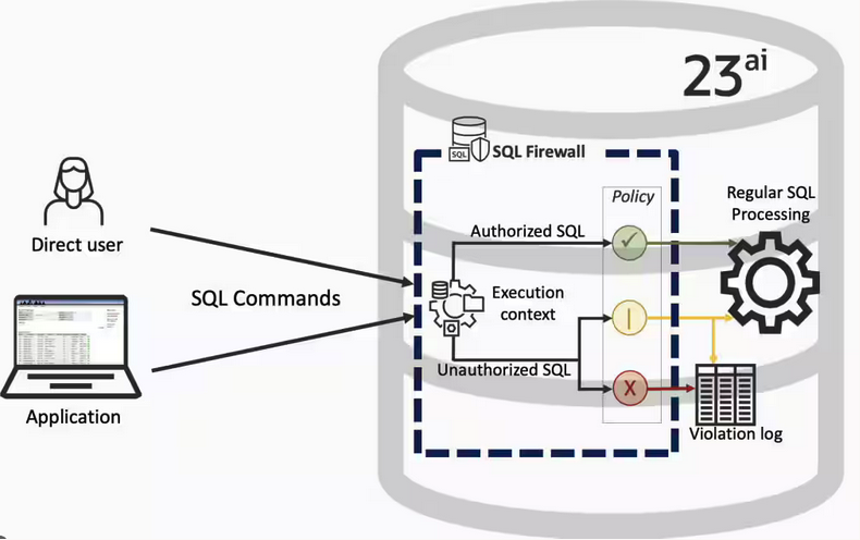
Typically, most IT architectures involve a firewall to act as a barrier, to monitor and to control network traffic. Its aim is to prevent unauthorised access and malicious activity. The firewall enforces rules to allow or block specific traffic (and commands/code). The firewall tries to protect our infrastructure and data. Over time, we have seen examples of how such firewalls have failed. We’ve also seen how our data (and databases) can be attacked internally. There are many ways to access the data and database without using the application. Many different people can have access to the data/database for many different purposes. There has been a growing need to push the idea of and the work of the firewall back to being closer to the data, that is, into the database.
SQL Firewall allows you to implement a firewall within the database to control what commands are allowed to be run on the data. With SQL Firewall you can:
- Monitor the SQL (and PL/SQL) activity to learn what the normal or typical SQL commands are being run on the data
- Captures all commands and logs them
- Manage a list of allowed commands, etc, using Policies
- Block and log all commands that are not allowed. Some commands might be allowed to run
Let’s walk through a simple example of setting this up and using it. For this example I’m assuming you have access to SYSTEM and another schema, for example SCOTT schema with the EMP, DEPT, etc tables.
Step 1 involves enabling SQL Firewall. To do this, we need to connect to the SYS schema and run the function to enable it.
grant sql_firewall_admin to system;Then connect to SYSTEM to enable the firewall.
exec dbms_sql_firewall.enable;For Step 2 we need to turn it on, as in we want to capture some of the commands being performed on the Database. We are using the SCOTT schema, so let’s capture what commands are run in that schema. [remember we are still connected to SYSTEM schema]
begin
  dbms_sql_firewall.create_capture (
    username=>'SCOTT',
    top_level_only=>true);
end;
Now that SQL Firewall is running, Step 3, we can switch to and connect to the SCOTT schema. When logged into SCOTT we can run some SQL commands on our tables.
select * from dept;
select deptno, count(*) from emp group by deptno;
select * from emp where job = 'MANAGER';
For Step 4, we can log back into SYSTEM and stop the capture of commands.
exec dbms_sql_firewall.stop_capture('SCOTT');We can then use the dictionary view DBA_SQL_FIREWALL_CAPTURE_LOG to see what commands were captured and logged.
column command_type format a12
column current_user format a15
column client_program format a45
column os_user format a10
column ip_address format a10
column sql_text format a30

select command_type,
       current_user,
       client_program,
       os_user,
       ip_address,
       sql_text
from   dba_sql_firewall_capture_logs
where  username = 'SCOTT';
The screen isn’t wide enough to display the results, but if you run the above command, you’ll see the three SELECT commands we ran above.
Other SQL Firewall dictionary views include DBA_SQL_FIREWALL_ALLOWED_IP_ADDR, DBA_SQL_FIREWALL_ALLOWED_OS_PROG, DBA_SQL_FIREWALL_ALLOWED_OS_USER and DBA_SQL_FIREWALL_ALLOWED_SQL.
For Step 5, we want to say that those commands are the only commands allowed in the SCOTT schema. We need to create an allowed list. Individual commands can be added, or if we want to add all the commands captured in our log, we can simple run
exec dbms_sql_firewall.generate_allow_list ('SCOTT');
exec  dbms_sql_firewall.enable_allow_list (username=>'SCOTT',block=>true);
Step 6 involves testing to see if the generated allowed list for SQL Firewall work. For this we need to log back into SCOTT schema, and run some commands. Let’s start with the three previously run commands. These should run without any problems or errors.
select * from dept;
select deptno, count(*) from emp group by deptno;
select * from emp where job = 'MANAGER';
Now write a different query and see what is returned.
select count(*) from dept;

Error starting at line : 1 in command -
select count(*) from dept
*
ERROR at line 1:
ORA-47605: SQL Firewall violation
Our new SQL command has been blocked. Which is what we wanted.
As an Administrator of the Database (DBA) you can monitor for violations of the Firewall. Log back into SYSTEM and run the following.
set lines 150
column occurred_at format a40

select sql_text,
       firewall_action,
       ip_address,
       cause,
       occurred_at
from   dba_sql_firewall_violations
where  username = 'SCOTT';

SQL_TEXT		       FIREWAL IP_ADDRESS CAUSE 	    OCCURRED_AT
------------------------------ ------- ---------- ----------------- ----------------------------------------
SELECT COUNT (*) FROM DEPT     Blocked 10.0.2.2   SQL violation     18-SEP-25 06.55.25.059913 PM +00:00
If you decide this command is ok to be run in the schema, you can add it to the allowed list.
exec dbms_sql_firewall.append_allow_list('SCOTT', dbms_sql_firewall.violation_log);The example above gives you the steps to get up and running with SQL Firewall. But there is lots more you can do with SQL Firewall, from monitoring of commands etc, to managing violations, to managing the logs, etc. Check out my other post covering some of these topics.
SQL History Monitoring
New in Oracle 23ai is a feature to allow tracking and monitoring the last 50 queries per session. Previously, we had other features and tools for doing this, but with SQL History we have some of this information in one location. SQL History will not replace what you’ve been using previously, but is just another tool to assist you in your monitoring and diagnostics. Each user can access their own current session history, while SQL and DBAs can view the history of all current user sessions.
If you want to use it, a user with ALTER SYTEM privilege must first change the initialisation parameter SQL_HISTORY_ENABLED instance wide to TRUE in the required PDB. The default is FALSE.
To see if it is enabled.
SELECT name,
       value,
       default_value,
       isdefault
FROM  v$parameter
WHERE name like 'sql_hist%';

NAME                 VALUE      DEFAULT_VALUE             ISDEFAULT
-------------------- ---------- ------------------------- ----------
sql_history_enabled  FALSE      FALSE                     TRUE
In the above example, the parameter is not enabled.
To enable the parameter, you need to do so using a user with SYSTEM level privileges. Use the ALTER SYSTEM privilege to enable it. For example,
alter system set sql_history_enabled=true scope=both;When you connect back to your working/developer schema you should be able to see the parameter has been enabled.
connect student/Password!@DB23

show parameter sql_history_enabled

NAME                            TYPE        VALUE
------------------------------- ----------- ------------------------------
sql_history_enabled             boolean     TRUE
A simple test to see it is working is to query the DUAL table
SELECT sysdate;

SYSDATE
---------
11-JUL-25
1 row selected.

SQL> select XYZ from dual;
select XYZ from dual
 *
ERROR at line 1:
ORA-00904: "XYZ": invalid identifier
Help: https://docs.oracle.com/error-help/db/ora-00904/
When we query the V$SQL_HISTORY view we get.
SELECT sql_text,
       error_number
FROM v$sql_history;

SQL_TEXT                                                ERROR_NUMBER
------------------------------------------------------- ------------
SELECT DECODE(USER, 'XS$NULL',  XS_SYS_CONTEXT('XS$SESS            0
SELECT sysdate                                                     0
SELECT xxx FROM dual                                             904
[I’ve truncated the SQL_TEXT above to fit on one line. By default, only the first 100 characters of the query are visible in this view]
This V$SQL_HISTORY view becomes a little bit more interesting when you look at some of the other columns that are available. in addition to the basic information for each statement like CON_ID, SID, SESSION_SERIAL#, SQL_ID and PLAN_HASH_VALUE, there are also lots of execution statistics like ELAPSED_TIME, CPU_TIME, BUFFER_GETS or PHYSICAL_READ_REQUESTS, etc. which will be of most interest.
The full list of columns is.
DESC v$sql_history

Name                                       Null?    Type
------------------------------------------ -------- -----------------------
 KEY                                                NUMBER
 SQL_ID                                             VARCHAR2(13)
 ELAPSED_TIME                                       NUMBER
 CPU_TIME                                           NUMBER
 BUFFER_GETS                                        NUMBER
 IO_INTERCONNECT_BYTES                              NUMBER
 PHYSICAL_READ_REQUESTS                             NUMBER
 PHYSICAL_READ_BYTES                                NUMBER
 PHYSICAL_WRITE_REQUESTS                            NUMBER
 PHYSICAL_WRITE_BYTES                               NUMBER
 PLSQL_EXEC_TIME                                    NUMBER
 JAVA_EXEC_TIME                                     NUMBER
 CLUSTER_WAIT_TIME                                  NUMBER
 CONCURRENCY_WAIT_TIME                              NUMBER
 APPLICATION_WAIT_TIME                              NUMBER
 USER_IO_WAIT_TIME                                  NUMBER
 IO_CELL_UNCOMPRESSED_BYTES                         NUMBER
 IO_CELL_OFFLOAD_ELIGIBLE_BYTES                     NUMBER
 SQL_TEXT                                           VARCHAR2(100)
 PLAN_HASH_VALUE                                    NUMBER
 SQL_EXEC_ID                                        NUMBER
 SQL_EXEC_START                                     DATE
 LAST_ACTIVE_TIME                                   DATE
 SESSION_USER#                                      NUMBER
 CURRENT_USER#                                      NUMBER
 CHILD_NUMBER                                       NUMBER
 SID                                                NUMBER
 SESSION_SERIAL#                                    NUMBER
 MODULE_HASH                                        NUMBER
 ACTION_HASH                                        NUMBER
 SERVICE_HASH                                       NUMBER
 IS_FULL_SQLTEXT                                    VARCHAR2(1)
 ERROR_SIGNALLED                                    VARCHAR2(1)
 ERROR_NUMBER                                       NUMBER
 ERROR_FACILITY                                     VARCHAR2(4)
 STATEMENT_TYPE                                     VARCHAR2(5)
 IS_PARALLEL                                        VARCHAR2(1)
CON_ID NUMBERVector Databases – Part 2
In this post on Vector Databases, I’ll look at the main components:
- Vector Embedding Models. What they do and what they create.
- Vectors. What they represent, and why they have different sizes.
- Vector Search. An overview of what a Vector Search will do. A more detailed version of this is in a separate post.
- Vector Search Process. It’s a multi-step process and some care is needed.

Vector Embedding Models
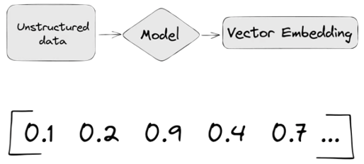
A vector embedding model is a type of machine learning model that transforms data into vectors (embeddings) in a high-dimensional space. These embeddings capture the semantic or contextual relationships between the data points, making them useful for tasks such as similarity search, clustering, and classification.
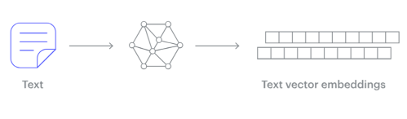
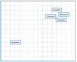
Embedding models are trained to convert the input data point (text, video, image, etc) into a vector (a series of numeric values). The model aims to identify semantic similarity with the input and map these to N-dimensional space. For example, the words “car” and “vehicle” have very different spelling but are semantically similar. The embedding model should map this to have similar vectors. Similarly with documents. The embedding model will map the documents to be able to group similar documents together (in N-dimensional space).
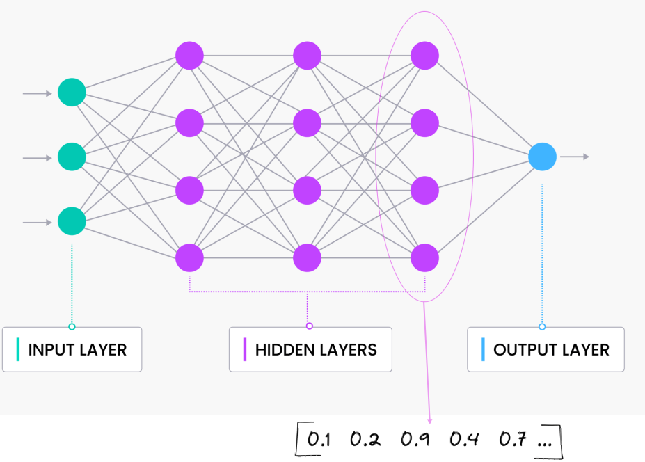
An embedding model is typically a Neural Network (NN) model. There are many different embedding models available from various vendor such as OpenAI, Cohere, etc., or you can build your own. Some models are open source and some are available for a fee. Typically, the output from the embedding model (the Vector) come from the last layer of the neural network
Vectors
A Vector is a sequence of numbers, called dimensions, used to capture the important “features” or “characteristics” of a piece of data. A vector is a mathematical object that has both magnitude (length) and direction. In the context of mathematics and physics, a vector is typically represented as an arrow pointing from one point to another in space, or as a list of numbers (coordinates) that define its position in a particular space.
Different Embedding Models create different numbers of Dimensions. Size is important with vectors as the greater the number number of dimensions the larger the Vector. The larger the number of dimensions the better the semantic similarity matches will be. As Vector size increases, so does space required to store them (not really a problem for Databases, but at Big Data scale it can be a challenge)
As vector size increases so does the Index space, and correspondingly search time can increase as the number of calculations for Distance Measure increases. There are various Vector indexes available to help with this (see my post covering this topic)
Basically, a vector is an array of numbers, where each number represents a dimension. It is easy for us to comprehend and visualise 2 dimensions. Here is an example of using 2 dimensions to represent different types of vehicles. The vectors give us a way to map or chart the data.
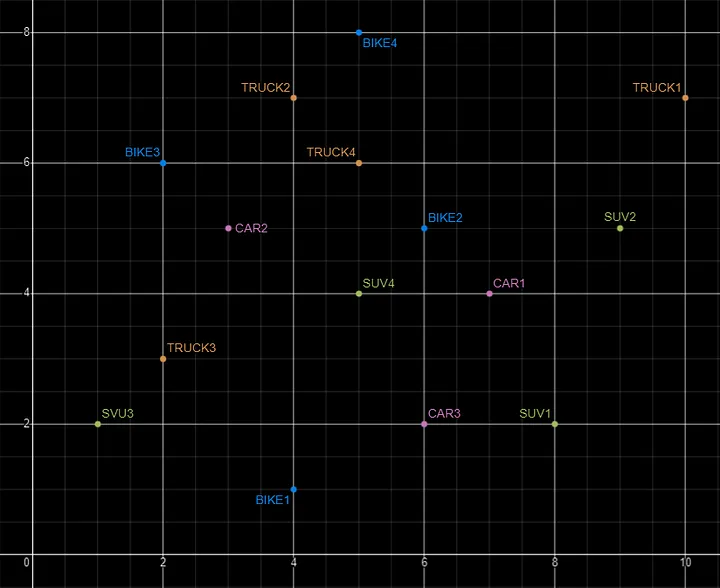
Here is SQL code for this data. I’ll come back to this data in the section on Vector Search.
INSERT INTO PARKING_LOT VALUES('CAR1','[7,4]');
INSERT INTO PARKING_LOT VALUES('CAR2','[3,5]');
INSERT INTO PARKING_LOT VALUES('CAR3','[6,2]');
INSERT INTO PARKING_LOT VALUES('TRUCK1','[10,7]');
INSERT INTO PARKING_LOT VALUES('TRUCK2','[4,7]');
INSERT INTO PARKING_LOT VALUES('TRUCK3','[2,3]');
INSERT INTO PARKING_LOT VALUES('TRUCK4','[5,6]');
INSERT INTO PARKING_LOT VALUES('BIKE1','[4,1]');
INSERT INTO PARKING_LOT VALUES('BIKE2','[6,5]');
INSERT INTO PARKING_LOT VALUES('BIKE3','[2,6]');
INSERT INTO PARKING_LOT VALUES('BIKE4','[5,8]');
INSERT INTO PARKING_LOT VALUES('SUV1','[8,2]');
INSERT INTO PARKING_LOT VALUES('SUV2','[9,5]');
INSERT INTO PARKING_LOT VALUES('SUV3','[1,2]');
INSERT INTO PARKING_LOT VALUES('SUV4','[5,4]');
The vectors created by the embedding models can have a different number of dimensions. Common Dimension Sizes are:
- 100-Dimensional: Often used in older or simpler models like some configurations of Word2Vec and GloVe. Suitable for tasks where computational efficiency is a priority and the context isn’t highly complex.
- 300-Dimensional: A common choice for many word embeddings (e.g., Word2Vec, GloVe). Strikes a balance between capturing sufficient detail and computational feasibility.
- 512-Dimensional: Used in some transformer models and sentence embeddings. Offers a richer representation than 300-dimensional embeddings.
- 768-Dimensional: Standard for BERT base models and many other transformer-based models. Provides detailed and contextual embeddings suitable for complex tasks.
- 1024-Dimensional: Used in larger transformer models (e.g., GPT-2 large). Provides even more detail but requires more computational resources.
Many of the newer embedding models have >3000 dimensions!
- Cohere’s embedding model embed-english-v3.0 has 1024 dimensions.
- OpenAI’s embedding model text-embedding-3-large has 3072 dimensions.
- Hugging Face’s embedding model all-MiniLM-L6-v2 has 384 dimensions
Here is a blog post listing some of the embedding models supported by Oracle Vector Search.
Vector Search
Vector search is a method of retrieving data by comparing high-dimensional vector representations (embeddings) of items rather than using traditional keyword or exact-match queries. This technique is commonly used in applications that involve similarity search, where the goal is to find items that are most similar to a given query based on their vector representations.
For example, using the vehicle data given above, we can easily visualise the search for similar vehicles. If we took “CAR1” as our initiating data point and wanted to know what other vehicles are similar to it. Vector Search looks at the distance between “CAR1” and all other vehicles in the 2-dimensional space.
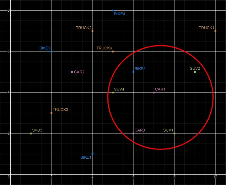
Vector Search becomes a bit more of a challenge when we have 1000+ dimensions, requiring advanced distance algorithms. I’ll have more on these in the next post.
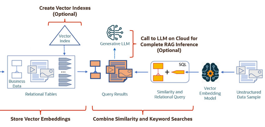
Vector Search Process
The Vector Search process is divided into two parts.
The first part involved creating Vectors for your existing data and for any new data generated and needs to be stored. This data can be used for Semantic Similarity searches (part two of the process). The first part of the process takes your data, applies a vector embedding model to it, generates the vectors and stores them in your Database. When the vectors are stored, Vector Indexes can be created.
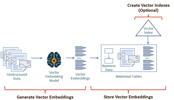
The second part if the process involves Vector Search. This involves having some data you want to search on (e.g. “CARS1” in the previous example). This data will need to be passed to the Vector Embedding model. A Vector for this data is generated. The Vector Search will use this vector to compare to all other vectors in the Database. The results returned will be those vectors (and their corresponding data) that closely match the vector being searched.
Check out my other posts in this series on Vector Databases.
Vector Databases – Part 1
A Vector Database is a specialized database designed to efficiently store, search, and retrieve high-dimensional vectors, which are often used to represent complex data like images, text, or audio. Vector Databases handle the growing need for managing unstructured and semi-structured data generated by AI models, particularly in applications such as recommendation systems, similarity search, and natural language processing. By enabling fast and scalable operations on vector embeddings, vector databases play a crucial role in unlocking the power of modern AI and machine learning applications.

While traditional Databases are very efficient with storing, processing and searching structured data, but over the past 10+ years they have expanded to include many of the typical NoSQL Database features. This allows ‘modern’ multi-model Databases to be capable of processing structured, semi-structured and unstructured data all within a single Database. Such NoSQL capabilities now available in ‘modern’ multi-model Databases include unstructured data, dynamic models, columnar data, in-memory data, distributed data, big data volumes, high performance, graph data processing, spatial data, documents, streaming, machine learning, artificial intelligence, etc. That is a long list of features and I haven’t listed everything. As new data processing paradigms emerge, they are evaluated and businesses identify the usefulness or not of each. If the new data processing paradigms are determined to be useful, apart from some niche use cases, these capabilities are integrated by the vendors of these ‘modern’ multi-model Database vendors. We have seen similar happen with Vector Databases over the past year or so. Yes Vector Databases have existed for many years but we now have the likes of Oracle, PostgreSQL, MySQL, SQL Server and even DB2 including Vector Embedding and Search.

Vector databases are specifically designed to store and search high-dimensional vector embeddings, which are generated by machine learning models. Here are some key use cases for vector databases:
1. Similarity Search:
- Image Search: Vector databases can be used to perform image similarity searches. For example, e-commerce platforms can allow users to search for products by uploading an image, and the system finds visually similar items using image embeddings.
- Document Search: In NLP (Natural Language Processing) tasks, vector databases help find semantically similar documents or text snippets by comparing their embeddings.
2. Recommendation Systems:
- Product Recommendations: Vector databases enable personalized product recommendations by comparing user and item embeddings to suggest items that are similar to a user’s past interactions or preferences.
- Content Recommendation: For media platforms (e.g., video streaming or news), vector databases power recommendation engines by finding content that matches the user’s interests based on embeddings of past behavior and content characteristics.
3. Natural Language Processing (NLP):
- Semantic Search: Vector databases are used in semantic search engines that understand the meaning behind a query, rather than just matching keywords. This is useful for applications like customer support or knowledge bases, where users may phrase questions in various ways.
- Question-Answering Systems: Vector databases can be employed to match user queries with relevant answers by comparing their vector representations, improving the accuracy and relevance of responses.
4. Anomaly Detection:
- Fraud Detection: In financial services, vector databases help detect anomalies or potential fraud by comparing transaction embeddings with a normal behavior profile.
- Security: Vector databases can be used to identify unusual patterns in network traffic or user behavior by comparing embeddings of normal activity to detect security threats.
5. Audio and Video Processing:
- Audio Search: Vector databases allow users to search for similar audio files or songs by comparing audio embeddings, which capture the characteristics of sound.
- Video Recommendation and Search: Embeddings of video content can be stored and queried in a vector database, enabling more accurate content discovery and recommendation in streaming platforms.
6. Geospatial Applications:
- Location-Based Services: Vector databases can store embeddings of geographical locations, enabling applications like nearest-neighbor search for finding the closest points of interest or users in a given area.
- Spatial Queries: Vector databases can be used in applications where spatial relationships matter, such as in logistics and supply chain management, where efficient searching of locations is crucial.
7. Biometric Identification:
- Face Recognition: Vector databases store face embeddings, allowing systems to compare and identify faces for authentication or security purposes.
- Fingerprint and Iris Matching: Similar to face recognition, vector databases can store and search biometric data like fingerprints or iris scans by comparing vector representations.
8. Drug Discovery and Genomics:
- Molecular Similarity Search: In the pharmaceutical industry, vector databases can help in searching for chemical compounds that are structurally similar to known drugs, aiding in drug discovery processes.
- Genomic Data Analysis: Vector databases can store and search genomic sequences, enabling fast comparison and clustering for research and personalized medicine.
9. Customer Support and Chatbots:
- Intelligent Response Systems: Vector databases can be used to store and retrieve relevant answers from a knowledge base by comparing user queries with stored embeddings, enabling more intelligent and context-aware responses in chatbots.
10. Social Media and Networking:
- User Matching: Social networking platforms can use vector databases to match users with similar interests, friends, or content, enhancing the user experience through better connections and content discovery.
- Content Moderation: Vector databases help in identifying and filtering out inappropriate content by comparing content embeddings with known examples of undesirable content.
These use cases highlight the versatility of vector databases in handling various applications that rely on similarity search, pattern recognition, and large-scale data processing in AI and machine learning environments.
This post is the first in a series on Vector Databases. Some will be background details and some will be technical examples using Oracle Database. I’ll post links to the following posts below as they are published.

You must be logged in to post a comment.