
database
SQL Firewall – Part 1
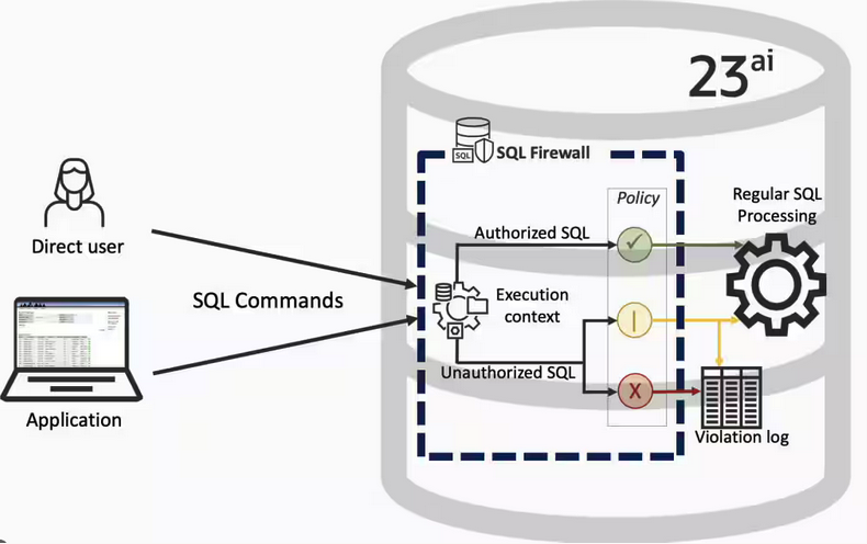
Typically, most IT architectures involve a firewall to act as a barrier, to monitor and to control network traffic. Its aim is to prevent unauthorised access and malicious activity. The firewall enforces rules to allow or block specific traffic (and commands/code). The firewall tries to protect our infrastructure and data. Over time, we have seen examples of how such firewalls have failed. We’ve also seen how our data (and databases) can be attacked internally. There are many ways to access the data and database without using the application. Many different people can have access to the data/database for many different purposes. There has been a growing need to push the idea of and the work of the firewall back to being closer to the data, that is, into the database.
SQL Firewall allows you to implement a firewall within the database to control what commands are allowed to be run on the data. With SQL Firewall you can:
- Monitor the SQL (and PL/SQL) activity to learn what the normal or typical SQL commands are being run on the data
- Captures all commands and logs them
- Manage a list of allowed commands, etc, using Policies
- Block and log all commands that are not allowed. Some commands might be allowed to run
Let’s walk through a simple example of setting this up and using it. For this example I’m assuming you have access to SYSTEM and another schema, for example SCOTT schema with the EMP, DEPT, etc tables.
Step 1 involves enabling SQL Firewall. To do this, we need to connect to the SYS schema and run the function to enable it.
grant sql_firewall_admin to system;Then connect to SYSTEM to enable the firewall.
exec dbms_sql_firewall.enable;For Step 2 we need to turn it on, as in we want to capture some of the commands being performed on the Database. We are using the SCOTT schema, so let’s capture what commands are run in that schema. [remember we are still connected to SYSTEM schema]
begin
  dbms_sql_firewall.create_capture (
    username=>'SCOTT',
    top_level_only=>true);
end;
Now that SQL Firewall is running, Step 3, we can switch to and connect to the SCOTT schema. When logged into SCOTT we can run some SQL commands on our tables.
select * from dept;
select deptno, count(*) from emp group by deptno;
select * from emp where job = 'MANAGER';
For Step 4, we can log back into SYSTEM and stop the capture of commands.
exec dbms_sql_firewall.stop_capture('SCOTT');We can then use the dictionary view DBA_SQL_FIREWALL_CAPTURE_LOG to see what commands were captured and logged.
column command_type format a12
column current_user format a15
column client_program format a45
column os_user format a10
column ip_address format a10
column sql_text format a30

select command_type,
       current_user,
       client_program,
       os_user,
       ip_address,
       sql_text
from   dba_sql_firewall_capture_logs
where  username = 'SCOTT';
The screen isn’t wide enough to display the results, but if you run the above command, you’ll see the three SELECT commands we ran above.
Other SQL Firewall dictionary views include DBA_SQL_FIREWALL_ALLOWED_IP_ADDR, DBA_SQL_FIREWALL_ALLOWED_OS_PROG, DBA_SQL_FIREWALL_ALLOWED_OS_USER and DBA_SQL_FIREWALL_ALLOWED_SQL.
For Step 5, we want to say that those commands are the only commands allowed in the SCOTT schema. We need to create an allowed list. Individual commands can be added, or if we want to add all the commands captured in our log, we can simple run
exec dbms_sql_firewall.generate_allow_list ('SCOTT');
exec  dbms_sql_firewall.enable_allow_list (username=>'SCOTT',block=>true);
Step 6 involves testing to see if the generated allowed list for SQL Firewall work. For this we need to log back into SCOTT schema, and run some commands. Let’s start with the three previously run commands. These should run without any problems or errors.
select * from dept;
select deptno, count(*) from emp group by deptno;
select * from emp where job = 'MANAGER';
Now write a different query and see what is returned.
select count(*) from dept;

Error starting at line : 1 in command -
select count(*) from dept
*
ERROR at line 1:
ORA-47605: SQL Firewall violation
Our new SQL command has been blocked. Which is what we wanted.
As an Administrator of the Database (DBA) you can monitor for violations of the Firewall. Log back into SYSTEM and run the following.
set lines 150
column occurred_at format a40

select sql_text,
       firewall_action,
       ip_address,
       cause,
       occurred_at
from   dba_sql_firewall_violations
where  username = 'SCOTT';

SQL_TEXT		       FIREWAL IP_ADDRESS CAUSE 	    OCCURRED_AT
------------------------------ ------- ---------- ----------------- ----------------------------------------
SELECT COUNT (*) FROM DEPT     Blocked 10.0.2.2   SQL violation     18-SEP-25 06.55.25.059913 PM +00:00
If you decide this command is ok to be run in the schema, you can add it to the allowed list.
exec dbms_sql_firewall.append_allow_list('SCOTT', dbms_sql_firewall.violation_log);The example above gives you the steps to get up and running with SQL Firewall. But there is lots more you can do with SQL Firewall, from monitoring of commands etc, to managing violations, to managing the logs, etc. Check out my other post covering some of these topics.
Annual Look at Database Trends (Jan 2024)
Each January I take a little time to look back on the Database market over the previous calendar year. This year I’ll have a look at 2023 (obviously!) and how things have changed and evolved.
In my post from last year (click here) I mentioned the behaviour of some vendors and how they like to be-little other vendors. That kind of behaviour is not really acceptable, but they kept on doing it during 2023 up to a point. That point occurred during the Autumn of 2023. It was during this period there was some degree of consolidation in the IT industry with staff reductions through redundancies, contracts not being renewed, and so on. These changes seemed to have an impact on the messages these companies were putting out and everything seemed to calm down. These staff reductions have continued into 2024.
The first half of the year was generally quiet until we reached the Summer. We then experienced a flurry of activity. The first was the release of the new SQL standard (SQL:2023). There were some discussions about the changes included (for example Property Graph Queries), but the news quickly fizzled out as SQL:2023 was primarily a maintenance release, where the standard was catching up on what many of the database vendors had already implemented over the preceding years. Two new topics seemed to take over the marketing space over the summer months and early autumn. These included LLMs and Vector Databases. Over the Autumn we have seen some releases across vendors incorporating various elements of these and we’ll see more during 2024. Although there have been a lot of marketing on these topics, it still remains to be seen what the real impact of these will be on your average, everyday type of enterprise application. In a similar manner to previous “new killer features” specialised database vendors, we are seeing all the mainstream database vendors incorporating these new features. Just like what has happened over the last 30 years, these specialised vendors will slowly or quickly disappear, as the multi-model database vendors incorporate the features and allow organisations to work with their database rather than having to maintain several different vendors. Another database topic that seemed to attract a lot of attention over the past few years was Distributed SQL (or previously called NewSQL). Again some of the activity around this topic and suppliers seemed to drop off in the second half of 2023. Time will tell what is happening here, maybe it is going through a similar time the NewSQL era had (the previous incarnation). The survivors of that era now call themselves Distributed SQL (Databases), which I think is a better name as it describes what they are doing more clearly. The size of this market is still relatively small. Again time will tell.
There was been some consolidation in the open source vendor market, with some mergers, buyouts, financial difficulties and some shutting down. There have been some high-profile cases not just from the software/support supplier side of things but also from the cloud hosting side of things. Not everyone and not every application can be hosted in the cloud, as Microsoft CEO reported in early 2023 that 90+% of IT spending is still for on-premises. We have also seen several reports and articles of companies reporting their exit from the Cloud (due to costs) and how much they have saved moving back to on-premises data centres.
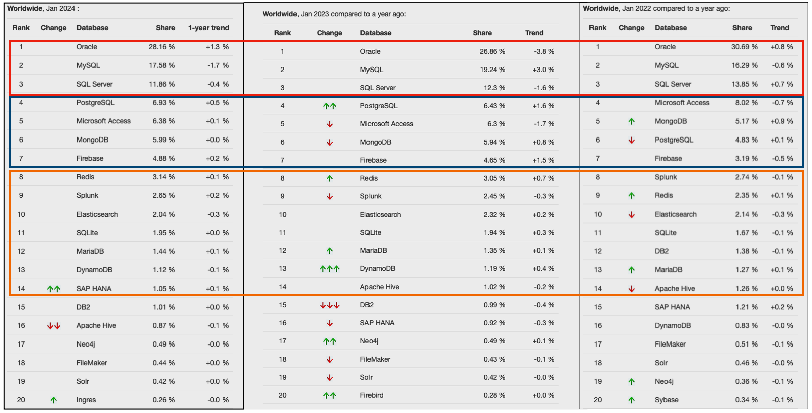
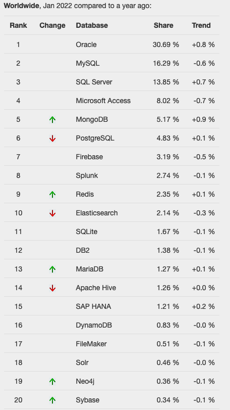
Two popular sites that constantly monitor the wider internet and judge how popular Databases are globally. These sites are DB-Engines and TOPDB Top Database index. These are well-known and are frequently cited. The image below, based on DB-Engines, shows the position of each Database in the top 20 and compares their position changes to 12 months previously. Here we have a comparison for 2023 and 2022 and the changes in positions. You’ll see there have been no changes in the positions of the top six Databases and minor positional changes for the next five Databases.

Although there has been some positive change for Postgres, given the numbers are based on log scale, this small change is small. The one notable mover in this table is Snowflake, which isn’t surprising really given what they offer and how they’ve been increasing their market share gradually over the years.
The TOPDB Top Database Index is another popular website and measures the popularity of Databases. It does this in a different way to DB-Engines. It can be an interesting exercise to cross-compare the results between the two websites. The image below compares the results from the past three years from TOPDB Top Database Index. We can see there is very little difference in the positions of most Databases. The point of interest here is the percentage Share of the top ten Databases. Have a look at the Databases that changed by more than one percentage point, and for those Databases (which had a lot of Marketing dollars) which moved very little, despite what some of their associated vendors try to get you to believe.
SQL:2023 Standard
As of June 2023 the new standard for SQL had been released, by the International Organization for Standards. Although SQL language has been around since the 1970s, this is the 11th release or update to the SQL standard. The first version of the standard was back in 1986 and the base-level standard for all databases was released in 1992 and referred to as SQL-92. That’s more than 30 years ago, and some databases still don’t contain all the base features in that standard, although they aim to achieve this sometime in the future.
| Year | Name | Alias | New Features or Enhancements |
|---|---|---|---|
| 1996 | SQL-86 | SQL-87 | This is the first version of the SQL standard by ANSI. Transactions, CREATE, Read, Update and Delete |
| 1989 | SQL-89 | This version includes minor revisions that added integrity constraints. | |
| 1992 | SQL-92 | SQL2 | This version includes major revisions on the SQL Language. Considered the base version of SQL. Many database systems, including NoSQL databases, use this standard for the base specification language, with varying degrees of implementation. |
| 1999 | SQL:1999 | SQL3 | This version introduces many new features such as regex matching, triggers, object-oriented features, OLAP capabilities and User Defined Types. The BOOLEAN data type was introduced but it took some time for all the major databases to support it. |
| 2003 | SQL:2003 | This version contained minor modifications to SQL:1999. SQL:2003 introduces new features such as window functions, columns with auto-generated values, identity specification and the addition of XML. | |
| 2006 | SQL:2006 | This version defines ways of importing, storing and manipulating XML data. Use of XQuery to query data in XML format. | |
| 2008 | SQL:2008 | This version includes major revisions to the SQL Language. Considered the base version of SQL. Many database systems, including NoSQL databases, use this standard for the base specification language, with varying degrees of implementation. | |
| 2011 | SQL:2011 | This version adds enhancements for window functions and FETCH clause, and Temporal data | |
| 2016 | SQL:2016 | This version adds various functions to work with JSON data and Polymorphic Table functions. | |
| 2019 | SQL:2019 | This version specifies muti-dimensional arrays data type. | |
| 2023 | SQL:2023 | This version contains minor updates to SQL functions to bring them in-line with how databases have implemented them. New JSON updates to include a new JSON data type with simpler dot notation processing. The main new addition to the standard is Property Graph Query (PDQ) which defines ways for the SQL language to represent property graphs and to interact with them. |
The Property Graph Query (PGQ) new features have been added as a new section or part of the standard and can be found labelled as Part-16: Property Graph Queries (SQL/PGQ). You can purchase the document for €191. Or you can read and scroll through the preview here.
For the other SQL updates, these updates were to reflect how the various (mainstream) database vendors (PostgreSQL, MySQL, Oracle, SQL Server, have implemented various functions. The standard is catching up with what is happening across the industry. This can be seen in some of the earlier releases
The following blog posts give a good overview of the SQL changes in the SQL:2023 standard.
Although SQL:2023 has been released there are some discussions about the next release of the standard. Although SQL:PGQ has been introduced, it also looks like (from various reports), some parts of SQL:PGQ were dropped and not included. More work is needed on these elements and will be included in the next release.
Also for the next release, there will be more JSON functionality included, with a particular focus on JSON Schemas. Yes, you read that correctly. There is a realisation that a schema is a good thing and when JSON objects can consist of up to 80% meta-data, a schema will have significant benefits for storage, retrieval and processing.
They are also looking at how to incorporate Streaming data. We can see some examples of this kind of processing in other languages and tools (Spark SQL, etc)
The SQL Standard is still being actively developed and we should see another update in a few years time.
Oracle 23c Free – Developer Release
Oracle 23c if finally available, in the form of Oracle 23c FREE – Developer Release. There was lots of excitement in some parts of the IT community about this release, some of which is to do with people having to wait a while for this release, given 22c was never released due to Covid!
But some caution is needed and reining back on the excitement is needed.

Why? This release isn’t the full bells and whistles full release of 23c Database. There has been several people from Oracle emphasizing the name of this release is Oracle 23c Free – Developer Release. There are a few things to consider with this release. It isn’t a GA (General Available) Release which is due later this year (maybe). Oracle 23c Free – Developer Release is an early release to allow developers to start playing with various developer focused new features. Some people have referred to this as the 23c Beta version 2 release, and this can be seen in the DB header information. It could be viewed in a similar way as the XE releases we had previously. XE was always Free, so we now we have a rename and emphasis of this. These have been many, many organizations using the XE release to build applications. Also the the XE releases were a no cost option, or what most people would like to say, the FREE version.
For the full 23c Database release we will get even more features, but most of these will probably be larger enterprise scale scenarios.
Now it’s time you to go play with 23c Free – Developer Release. Here are some useful links
- Product Release Official Announcement
- Post by Gerald Venzi
- See link for Docker installation below
- VirtualBox Virtual Machine
- You want to do it old school – Download RPM files
- New Features Guide
I’ll be writing posts on some of the more interesting new features and I’ll add the links to those below. I’ll also add some links to post by other people:
- Docker Installation (Intel and Apple Chip)
- 23 Free Virtual Machine
- 23 Free – A Few (New Features) A few Quickies
- JSON Relational Duality – see post by Tim Hall
- more coming soon (see maintained list at https://oralytics.com/23c/)
Annual Look at Database Trends (Jan 2023)
Monitoring trends in the popularity and usage of different Database vendors can be a interesting exercise. The marketing teams from each vendor do an excellent job of promoting their Database, along with the sales teams, developer advocates, and the user communities. Some of these are more active than others and it varies across the Database market on what their choice is for promoting their products. One of the problems with these various types of marketing, is how can be believe what they are saying about how “awesome” their Database is, and then there are some who actively talk about how “rubbish” (or saying something similar) other Databases area. I do wonder how this really works for these people and vendors when to go negative about their competitors. A few months ago I wrote about “What does Legacy Really Mean?“. That post was prompted by someone from one Database Vendor calling their main competitor Database a legacy product. They are just name calling withing providing any proof or evidence to support what they are saying.
Getting back to the topic of this post, I’ve gathered some data and obtained some league tables from some sites. These will help to have a closer look at what is really happening in the Database market throughout 2022. Two popular sites who constantly monitor the wider internet and judge how popular Databases area globally. These sites are DB-Engines and TOPDB Top Database index. These are well know and are frequently cited. Both of these sites give some details of how they calculate their scores, with one focused mainly on how common the Database appears in searches across different search engines, while the other one, in addition to search engine results/searches, also looks across different websites, discussion forms, social media, job vacancies, etc.
The first image below is a comparison of the league tables from DB-Engines taken in January 2022 and January 2023. I’ve divided this image into three sections/boxes. Overall for the first 10 places, not a lot has changed. The ranking scores have moved slightly in most cases but not enough to change their position in the rank. Even with a change of score by 30+ points is a very small change and doesn’t really indicate any great change in the score as these scores are ranked in a manner where, “when system A has twice as large a value in the DB-Engines Ranking as system B, then it is twice as popular when averaged over the individual evaluation criteria“. Using this explanation, Oracle would be twice as popular when compared to PostgreSQL. This is similar across 2022 and 2023.

Next we’ll look a ranking from TOPDB Top Database index. The image below compares January 2022 and January 2023. TOPDB uses a different search space and calculation for its calculation. The rankings from TOPDB do show some changes in the ranks and these are different to those from DB-Engines. Here we see the top three ranks remain the same with some small percentage changes, and nothing to get excited about. In the second box covering ranks 4-7 we do some changes with PostgreSQL improving by two position and MongoDB. These changes do seem to reflect what I’ve been seeing in the marketplace with MongoDB being replaced by PostgreSQL and MySQL, with this multi-model architecture where you can have relational, document, and other data models in the one Database. It’s important to note Oracle and SQL Server also support this. Over the past couple of years there has been a growing awareness of and benefits of having relation and document (and others) data models in the one database. This approach makes sense both for developer productivity, and for data storage and management.

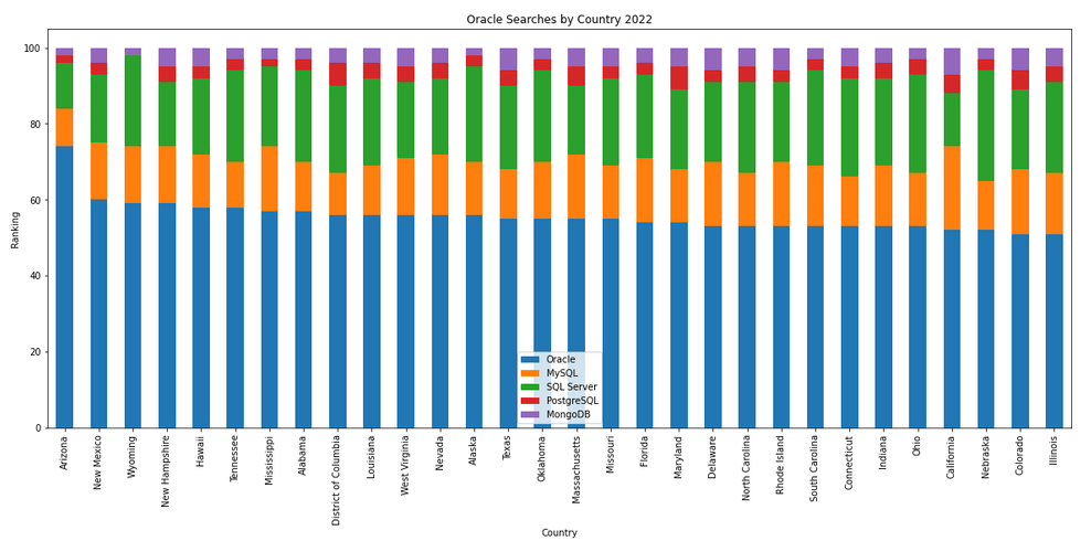
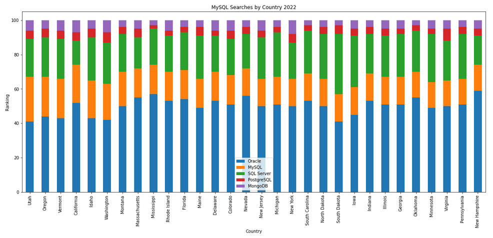
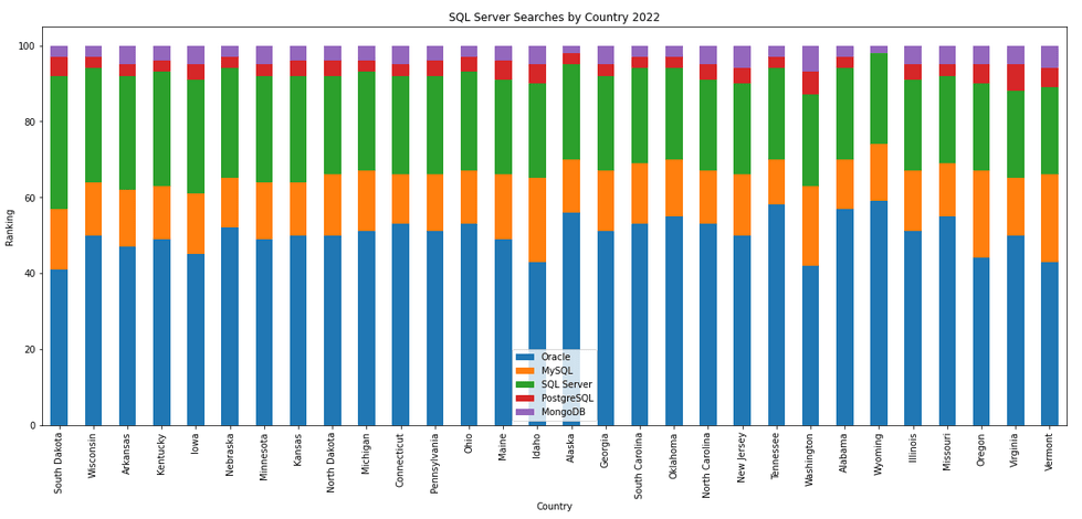
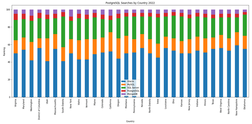
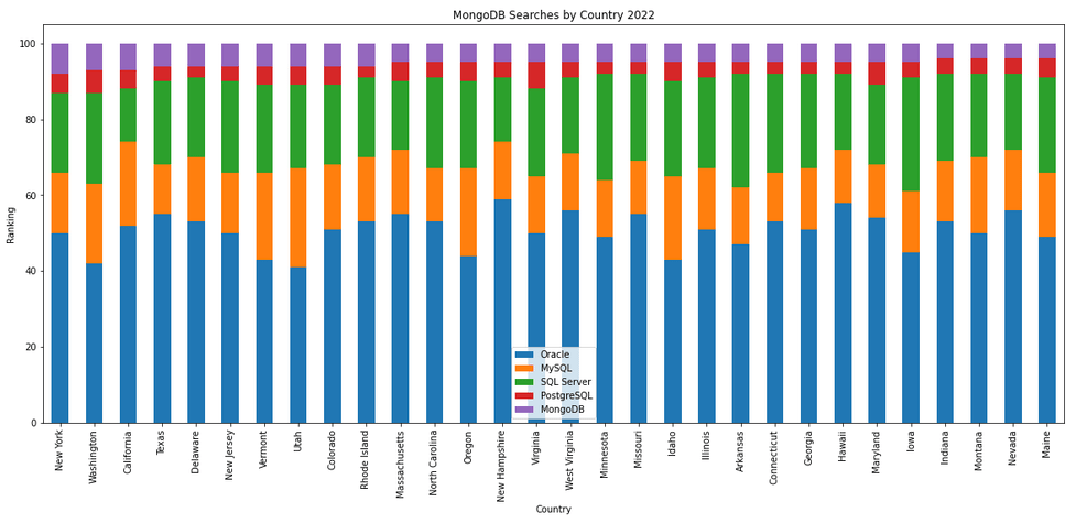
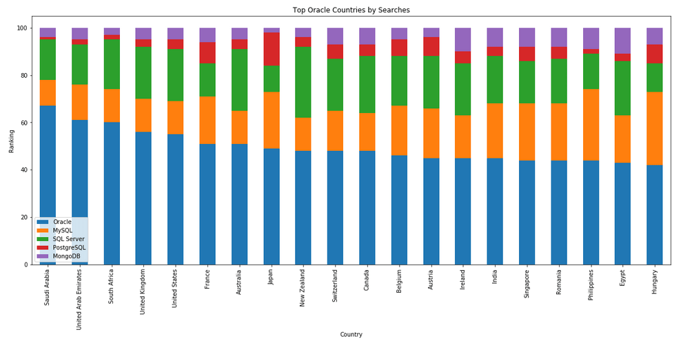
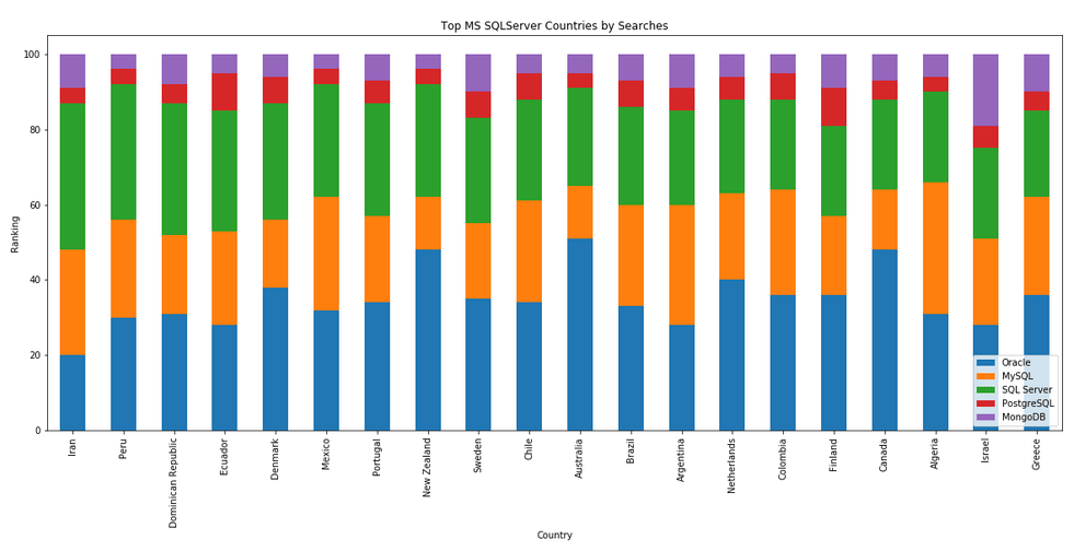
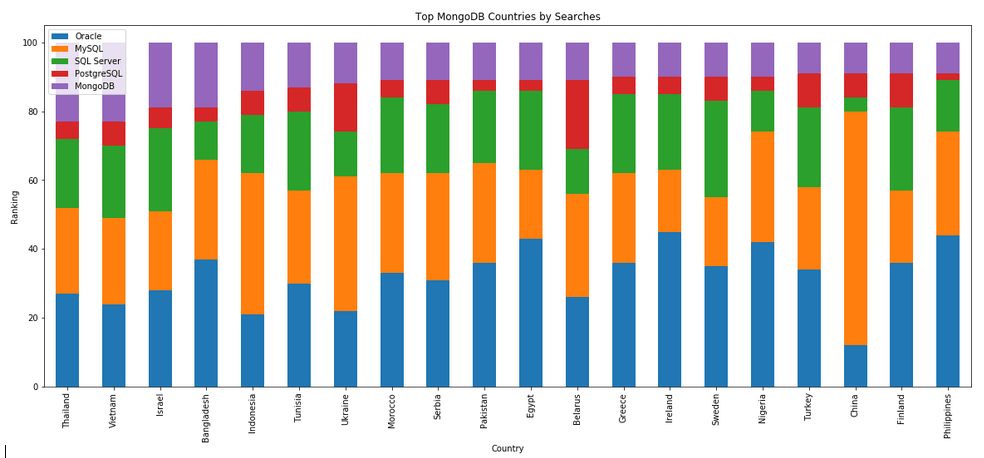
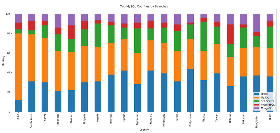
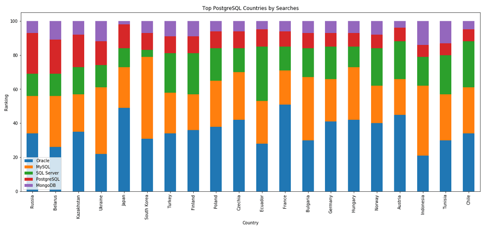
The next gallery of images is based on some Python code I’ve written to look a little bit closer at the top five Databases. In this case these are Oracle, MySQL, SQL Server, PostgreSQL and MongoDB. This gallery plots a bar chart for each Database for their top 15 Counties, and compares them with the other four Databases. The results are interesting and we can see some geographic aspects to the popularity of the Databases.
What does Legacy really mean?
In the IT industry we hear the term “legacy” being using, but that does it mean? It can mean a lot of different things and it really depends on the person who is saying it, their context, what they want to portray and their intended meaning. In a lot of cases people seem to use it without knowing the meaning or the impact it can have. This can result in negative impact and not in the way the person intended.
Before looking at some (and there can be lots) possible meanings, lets have a look at what one person said recently.
“Migrating away from legacy databases like Oracle can seem like a daunting undertaking for businesses. But it doesn’t have to be.”
To give context to this quote, the person works for a company selling products, services, support, etc for PostgreSQL and wants everyone to move to ProtgreSQL (Postgres), which is understandable given their role. There’s nothing wrong with trying to convince people/companies to use software that you sell lots of services and additional software to support it. What is interesting is they used the work “legacy”.
Legacy can mean lots of different things to different people. Here are some examples of how legacy is used within the IT industry.
- The product is old and out of date
- The product has no relevancy in software industry today
- Software or hardware that has been superseded
- Any software that has just been released (yes I’ve come across this use)
- Outdated computing software and/or hardware that is still in use. The system still meets the needs it was originally designed for, but doesn’t allow for growth
- Anything in production
- Software that has come to an end of life with no updates, patching and/or no product roadmap
- …
Going back to the quote given above, let’s look a little closer at their intended use. As we can see from the list above the use of the word “legacy” can be used in derogatory way and can try to make one software appear better then it’s old, out of date, not current, hard to use, etc competitor.
If you were to do a side-by-side comparison of PostgreSQL and Oracle, there would be a lot of the same or very similar features. But there are differences too and this, in PostgreSQL case, we see various vendors offering add-on software you can pay for. This is kind of similar with Oracle where you need to license various add-ons, or if you are using a Cloud offering it may come as part of the package. On a features comparison level when these are similar, saying one is “legacy” doesn’t seem right. Maybe its about how old the software is, as in legacy being old software. The first release of Oracle was 1979 and we now get yearly update releases (previously it could be every 2-4 years). PostgresSQL, or its previous names date back to 1974 with the first release of Ingres, which later evolved to Postgres in early 1980s, and took on the new name of PostgreSQL in 1996. Are both products today still the same as what they had in the 1970s, 1980s, 1990s, etc. The simple answer is No, they have both evolved and matured since then. Based on this can we say PostgreSQL is legacy or is more of a Legacy product than Oracle Database which was released in 1979 (5 years after Ingres)? Yes we can.
I’m still very confused by the quote (given above) as to what “legacy” might mean, in their scenario. Apart from and (trying) to ignore the derogatory aspect of “they” are old and out of date, and look at us we are new and better, it is difficult to see what they are trying to achieve.
In a similar example on a LinkedIn discussion where one person said MongoDB was legacy, was a little surprising. MongoDB is very good at what it does and has a small number of use cases. The problem with MongoDB is it is used in scenarios when it shouldn’t be used and just causes too many data architecture problems. For me, the main problem driving these issues is how software engineering and programming is taught in Universities (and other third level institutions). They are focused on JavaScript which makes using MongoDB so so easy. And its’ Agile, and the data model can constantly change. This is great, up until you need to use that data. Then it becomes a nightmare.
Getting back to saying MongoDB is legacy, again comes back to the person saying it. They work at a company who is selling cloud based data engineering and analytic services. Is using cloud services the only thing people should be using? For me it is No but a hybrid cloud and on-premises approach will work based for most. Some of the industry analysts are now promoting this, saying vendors offering both will succeed into the future, where does only offering cloud based services will have limited growth, unless the adapt now.
What about other types legacy software applications. Here is an example Stew Ashton posted on Twitter. “I once had a colleague who argued, in writing, that changing the dev stack had the advantage of forcing a rewrite of “legacy applications” – which he had coded the previous year! Either he thought he had greatly improved, or he wanted guaranteed job security”
There are lots and lots of more examples out there and perhaps you will encounter some when you are attending presentations or sales pitches from various vendors. If you hear, then saying one product is “legacy” get them to define their meaning of it and to give specific examples to illustrate it. Does their meaning match with one from the list given above, or something else. Are they just using the word to make another product appear inferior without knowing the meaning or the differences in the product? Their intended meaning within their context is what defines their meaning, which may be different to yours.
AUTO_PARTITION – Inspecting & Implementing Recommendations
In a previous blog post I gave an overview of the DBMS_AUTO_PARTITION package in Oracle Autonomous Database. This looked at how you can get started and to setup Auto Partitioning and to allow it to automatically implement partitioning.
This might not be something the DBAs will want to happen for lots of different reasons. An alternative is to use DBMS_AUTO_PARTITION to make recommendations for tables where partitioning will have a performance improvement. The DBA can inspect these recommendations and decide which of these to implement.
In the previous post we set the CONFIGURE function to be ‘IMPLEMENT’. We need to change that to report the recommendations.
exec dbms_auto_partition.configure('AUTO_PARTITION_MODE','REPORT ONLY');Just remember, tables will only be considered by AUTO_PARTITION as outlined in my previous post.
Next we can ask for recommendations using the RECOMMEND_PARTITION_METHOD function.
exec  dbms_auto_partition.recommend_partition_method(
   table_owner => 'WHISKEY',
   table_name => 'DIRECTIONS',
   report_type => 'TEXT',
   report_section => 'ALL',
   report_level => 'ALL');
The results from this are stored in DBA_AUTO_PARTITION_RECOMMENDATIONS, which you can query to view the recommendations.
select recommendation_id, partition_method, partition_key
from dba_auto_partition_recommendations;
RECOMMENDATION_ID PARTITION_METHOD PARTITION_KEY
-------------------------------- ------------------------------------------------------------------------------------------------------------- --------------
D28FC3CF09DF1E1DE053D010000ABEA6 Method: LIST(SYS_OP_INTERVAL_HIGH_BOUND("D", INTERVAL '2' MONTH, TIMESTAMP '2019-08-10 00:00:00')) AUTOMATIC D
To apply the recommendation pass the RECOMMENDATION_KEY value to the APPLY_RECOMMENDATION function.
exec dbms_auto_partition.apply_recommendation('D28FC3CF09DF1E1DE053D010000ABEA6');It might takes some minutes for the partitioned table to become available. During this time the original table will remain available as the change will be implemented using a ALTER TABLE MODIFY PARTITION ONLINE command.
Two other functions include REPORT_ACTIVITY and REPORT_LAST_ACTIVITY. These can be used to export a detailed report on the recommendations in text or HTML form. It is probably a good idea to create and download these for your change records.
spool autoPartitionFinding.html
select dbms_auto_partition.report_last_activity(type=>'HTML') from dual;
exit;AUTO_PARTITION – Basic setup
Partitioning is an effective way to improve performance of SQL queries on large volumes of data in a database table. But only so, if a bit of care and attention is taken by both the DBA and Developer (or someone with both of these roles). Care is needed on the database side to ensure the correct partitioning method is deployed and the management of these partitions, as some partitioning methods can create a significantly large number of partitions, which in turn can affect the management of these and possibly performance too, which is not what you want. Care is also needed from the developer side to ensure their code is written in a way that utilises the partitioning method deployed. If doesn’t then you may not see much improvement in performance of your queries, and somethings things can run slower. Which not one wants!
With the Oracle Autonomous Database we have the expectation it will ‘manage’ a lot of the performance features behind the scenes without the need for the DBA and Developing getting involved (‘Autonomous’). This is kind of true up to a point, as the serverless approach can work up to a point. Sometimes a little human input is needed to give a guiding hand to the Autonomous engine to help/guide it towards what data needs particular focus.
In this (blog post) case we will have a look at DBMS_AUTO_PARTITION and how you can do a basic setup, config and enablement. I’ll have another post that will look at the recommendation feature of DBMS_AUTO_PARTITION. Just a quick reminder, DBMS_AUTO_PARTITION is for the Oracle Autonomous Database (ADB) (on the Cloud). You’ll need to run the following as ADMIN user.
The first step is to enable auto partitioning on the ADB using the CONFIGURE function. This function can have three parameters:
- IMPLEMENT : generates a report and implements the recommended partitioning method. (Autonomous!)
- REPORT_ONLY : {default} reports recommendations for partitioning on tables
- OFF : Turns off auto partitioning (reporting and implementing)
For example, to enable auto partitioning and to automatically implement the recommended partitioning method.
exec DBMS_AUTO_PARTITION.CONFIGURE('AUTO_PARTITION_MODE', 'IMPLEMENT');The changes can be inspected in the DBA_AUTO_PARTITION_CONFIG view.
SELECT * FROM DBA_AUTO_PARTITION_CONFIG;When you look at the listed from the above select we can see IMPLEMENT is enabled

The next step with using DBMS_AUTO_PARTITION is to tell the ADB what schemas and/or tables to include for auto partitioning. This first example shows how to turn on auto partitioning for a particular schema, and to allow the auto partitioning (engine) to determine what is needed and to just go and implement that it thinks is the best partitioning methods.
exec DBMS_AUTO_PARTITION.CONFIGURE(
   parameter_name => 'AUTO_PARTITION_SCHEMA',
   parameter_value => 'WHISKEY',
   ALLOW => TRUE);
If you query the DBA view again we now get.
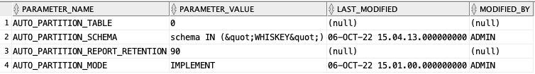
We have not enabled a schema (called WHISKEY) to be included as part of the auto partitioning engine.
Auto Partitioning may not do anything for a little while, with some reports suggesting to wait for 15 minutes for the database to pick up any changes and to make suggestions. But there are some conditions for a table needs to meet before it can be considered, this is referred to as being a ‘Candidate’. These conditions include:
- Table passes inclusion and exclusion tests specified by AUTO_PARTITION_SCHEMA and AUTO_PARTITION_TABLE configuration parameters.
- Table exists and has up-to-date statistics.
- Table is at least 64 GB.
- Table has 5 or more queries in the SQL tuning set that scanned the table.
- Table does not contain a LONG data type column.
- Table is not manually partitioned.
- Table is not an external table, an internal/external hybrid table, a temporary table, an index-organized table, or a clustered table.
- Table does not have a domain index or bitmap join index.
- Table is not an advance queuing, materialized view, or flashback archive storage table.
- Table does not have nested tables, or certain other object features.
If you find Auto Partitioning isn’t partitioning your tables (i.e. not a valid Candidate) it could be because the table isn’t meeting the above list of conditions.
This can be verified using the VALIDATE_CANDIDATE_TABLE function.
select DBMS_AUTO_PARTITION.VALIDATE_CANDIDATE_TABLE(
   table_owner => 'WHISKEY',
   table_name => 'DIRECTIONS')
from dual;
If the table has met the above list of conditions, the above query will return ‘VALID’, otherwise one or more of the above conditions have not been met, and the query will return ‘INVALID:’ followed by one or more reasons
Check out my other blog post on using the AUTO_PARTITION to explore it’s recommendations and how to implement.
Postgres on Docker
Prostgres is one of the most popular databases out there, being used in Universities, open source projects and also widely used in the corporate marketplace. I’ve written a previous post on running Oracle Database on Docker. This post is similar, as it will show you the few simple steps to have a persistent Postgres Database running on Docker.
The first step is go to Docker Hub and locate the page for Postgres. You should see something like the following. Click through to the Postgres page.

There are lots and lots of possible Postgres images to download and use. The simplest option is to download the latest image using the following command in a command/terminal window. Make sure Docker is running on your machine before running this command.
docker pull postgresAlthough, if you needed to install a previous release, you can do that.

After the docker image has been downloaded, you can now import into Docker and create a container.
docker run --name postgres -p 5432:5432 -e POSTGRES_USER=postgres -e POSTGRES_PASSWORD=pgPassword -e POSTGRES_DB=postgres -d postgresImportant: I’m using Docker on a Mac. If you are using Windows, the format of the parameter list is slightly different. For example, remove the = symbol after POSTGRES_DB
If you now check with Docker you’ll see Postgres is now running on post 5432.

Next you will need pgAdmin to connect to the Postgres Database and start working with it. You can download and install it, or run another Docker container with pgAdmin running in it.
First, let’s have a look at installing pgAdmin. Download the image and run, accepting the initial requirements. Just let it run and finish installing.


When pgAdmin starts it looks for you to enter a password. This can be anything really, but one that you want to remember. For example, I set mine to pgPassword.
Then create (or Register) a connection to your Postgres Database. Enter the details you used when creating the docker image including username=postgres, password=pgPassword and IP address=0.0.0.0.
The IP address on your machine might be a little different, and to check what it is, run the following
docker ps -a


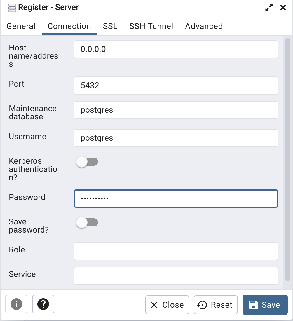
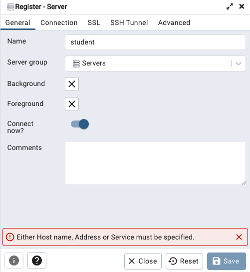
When your (above) connection works, the next step is to create another schema/user in the database. The reason we need to do this is because the user we connected to above (postgres) is an admin user. This user/schema should never be used for database development work.
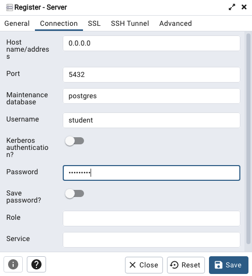
Let’s setup a user we can use for our development work called ‘student’. To do this, right click on the ‘postgres’ user connection and open the query tool.
Then run the following.

After these two commands have been run successfully we can now create a connection to the postgres database, open the query tool and you’re now all set to write some SQL.

Oracle Database In-Memory – simple example
In a previous post, I showed how to enable and increase the memory allocation for use by Oracle In-Memory. That example was based on using the Pre-built VM supplied by Oracle.
To use In-Memory on your objects, you have a few options.
Enabling the In-Memory attribute on the EXAMPLE tablespace by specifying the INMEMORY attribute
SQL> ALTER TABLESPACE example INMEMORY;Enabling the In-Memory attribute on the sales table but excluding the “prod_id” column
SQL> ALTER TABLE sales INMEMORY NO INMEMORY(prod_id);Disabling the In-Memory attribute on one partition of the sales table by specifying the NO INMEMORY clause
SQL> ALTER TABLE sales MODIFY PARTITION SALES_Q1_1998 NO INMEMORY;Enabling the In-Memory attribute on the customers table with a priority level of critical
SQL> ALTER TABLE customers INMEMORY PRIORITY CRITICAL;You can also specify the priority level, which helps to prioritise the order the objects are loaded into memory.

A simple example to illustrate the effect of using In-Memory versus not.
Create a table with, say, 11K records. It doesn’t really matter what columns and data are.
Now select all the records and display the explain plan
select count(*) from test_inmemory;
Now, move the table to In-Memory and rerun your query.
alter table test_inmemory inmemory PRIORITY critical;
select count(*) from test_inmemory;  -- again
There you go!
We can check to see what object are In-Memory by
SELECT table_name, inmemory, inmemory_priority, inmemory_distribute,
       inmemory_compression, inmemory_duplicate
FROM user_tables
WHERE inmemory = 'ENABLED’
ORDER BY table_name;
To remove the object from In-Memory
SQL > alter table test_inmemory no inmemory; -- remove the table from in-memory
This is just a simple test and lots of other things can be done to improve performance
But, you do need to be careful about using In-Memory. It does have some limitations and scenarios where it doesn’t work so well. So care is needed
Changing In-Memory size in Oracle Database
The pre-built virtual machine provided by Oracle for trying out and playing with Oracle Database comes configured to use the In-Memory option. But memory size is a little limited if you are trying to load anything slightly bigger than a tiny table into memory, for example if the table has more than a few hundred rows.
The amount of memory allocated to In-Memory can be increased to allow for more data to be loaded. There is a requirement that the VM and Database has enough memory allocated to allow this. If you don’t and increase the In-Memory size too large, you will have some problems restarting the database and VM. So proceed carefully.
For the pre-built VM, I typically allocate 4G or 8G of RAM to the VM. This in turn will give more memory to the database when it starts.
To setup In-Memory on the VM run the following:
– Open a terminal window and run this command:
sqlplus sys/oracle as sysdbaThen run these two commands
alter session set container = cdb$root;
alter system set inmemory_size = 200M scope=spfile;
Now, bounce the VM, i.e. restart the VM
In-memory will now be enabled on your Database, and you can now create/move tables in and out of in-memory.
Database Vendors on Twitter, Slack, downloads, etc.
Each year we see some changes in the positioning of the most popular databases on the market. “The most popular” part of that sentence can be the most difficult to judge. There are lots and lots of different opinions on this and ways of judging them. There are various sites giving league tables, and even with those some people don’t agree with how they perform their rankings.
The following table contains links for some of the main Database engines including download pages, social media links, community support sites and to the documentation.
One of the most common sites is DB-Engines, and another is TOPDB Top Database index. The images below show the current rankings/positions of the database vendors (in January 2022).
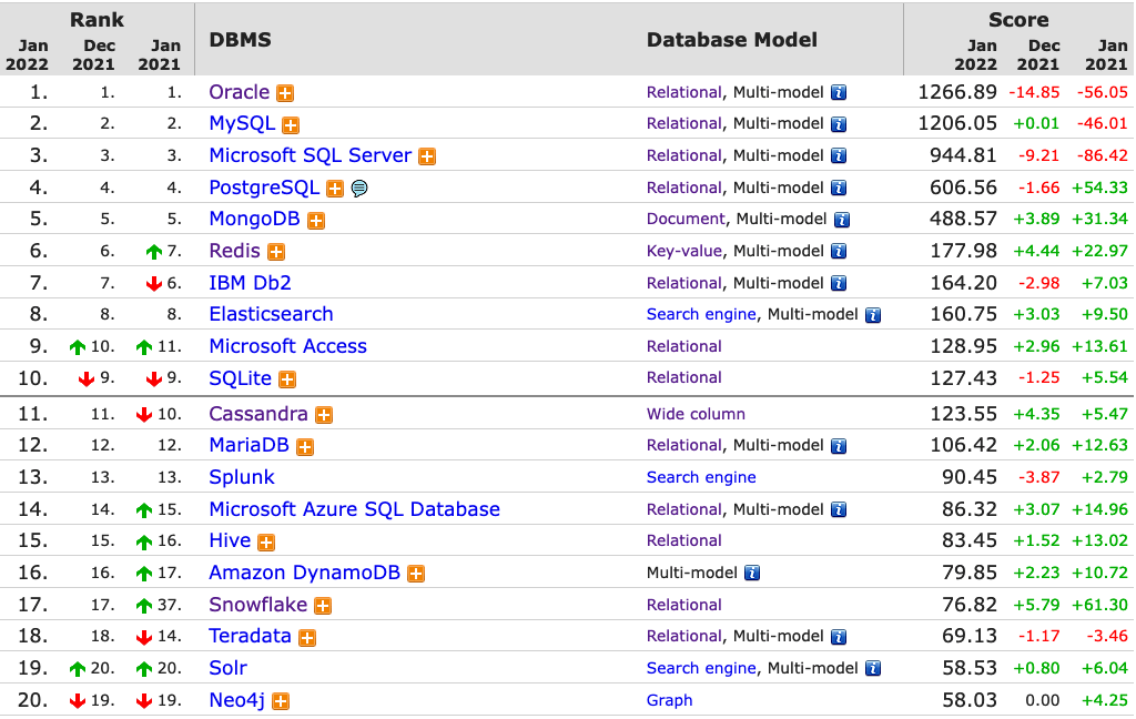
I’ve previously written about using the Python pytrends package to explore the relative importance of the different Database engines. The results from pytrends gives results based on number of searches etc in Google. Check out that Blog Post. I’ve rerun the same code for 2021, and the following gallery displays charts for each Database based on their popularity. This will allow you to see what countries are most popular for each Database and how that relates to the other databases. For these charts I’ve included Oracle, MySQL, SQL Server, PostgreSQL and MongoDB, as these are the top 5 Databases from DB-Engines.

You must be logged in to post a comment.