
Oracle
What a difference a Bind Variable makes
To bind or not to bind, that is the question?
Over the years, I heard and read about using Bind variables and how important they are, particularly when it comes to the efficient execution of queries. By using bind variables, the optimizer will reuse the execution plan from the cache rather than generating it each time. Recently, I had conversations about this with a couple of different groups, and they didn’t really believe me and they asked me to put together a demonstration. One group said they never heard of ‘prepared statements’, ‘bind variables’, ‘parameterised query’, etc., which was a little surprising.
The following is a subset of what I demonstrated to them to illustrate the benefits and potential benefits.
Here is a basic example of a typical scenario where we have a SQL query being constructed using concatenation.
select * from order_demo where order_id = || 'i';That statement looks simple and harmless. When we try to check the EXPLAIN plan from the optimizer we will get an error, so let’s just replace it with a number, because that’s what the query will end up being like.
select * from order_demo where order_id = 1;When we check the Explain Plan, we get the following. It looks like a good execution plan as it is using the index and then doing a ROWID lookup on the table. The developers were happy, and that’s what those recent conversations were about and what they are missing.
-------------------------------------------------------------
| Id  | Operation                   | Name         | E-Rows |
-------------------------------------------------------------
|   0 | SELECT STATEMENT            |              |        |
|   1 |  TABLE ACCESS BY INDEX ROWID| ORDER_DEMO   |      1 |
|*  2 |   INDEX UNIQUE SCAN         | SYS_C0014610 |      1 |
-------------------------------------------------------------
The missing part in their understanding was what happens every time they run their query. The Explain Plan looks good, so what’s the problem? The problem lies with the Optimizer evaluating the execution plan every time the query is issued. But the developers came back with the idea that this won’t happen because the execution plan is cached and will be reused. The problem with this is how we can test this, and what is the alternative, in this case, using bind variables (which was my suggestion).
Let’s setup a simple test to see what happens. Here is a simple piece of PL/SQL code which will look 100K times to retrieve just one row. This is very similar to what they were running.
DECLARE
   start_time TIMESTAMP;
   end_time   TIMESTAMP;
BEGIN
   start_time := systimestamp;
   dbms_output.put_line('Start time : ' || to_char(start_time,'HH24:MI:SS:FF4'));
   --
   for i in 1 .. 100000 loop
      execute immediate 'select * from order_demo where order_id = '||i;
   end loop;
   --
   end_time := systimestamp;
   dbms_output.put_line('End time : ' || to_char(end_time,'HH24:MI:SS:FF4'));
END;
/
When we run this test against a 23.7 Oracle Database running in a VM on my laptop, this completes in little over 2 minutes
Start time : 16:26:04:5527
End time : 16:28:13:4820


PL/SQL procedure successfully completed.

Elapsed: 00:02:09.158
The developers seemed happy with that time! Ok, but let’s test it using bind variables and see if it’s any different. There are a few different ways of setting up bind variables. The PL/SQL code below is one example.
DECLARE
   order_rec  ORDER_DEMO%rowtype;
   start_time TIMESTAMP;
   end_time   TIMESTAMP;
BEGIN
   start_time := systimestamp;
   dbms_output.put_line('Start time : ' || to_char(start_time,'HH24:MI:SS:FF9'));
   --
   for i in 1 .. 100000 loop
   execute immediate 'select * from order_demo where order_id = :1' using i;
	end loop;
	--
    end_time := systimestamp;
    dbms_output.put_line('End time : ' || to_char(end_time,'HH24:MI:SS:FF9'));
END;
/
Start time : 16:31:39:162619000
End time : 16:31:40:479301000


PL/SQL procedure successfully completed.

Elapsed: 00:00:01.363
This just took a little over one second to complete. Let me say that again, a little over one second to complete. We went from taking just over two minutes to run, down to just over one second to run.
The developers were a little surprised or more correctly, were a little shocked. But they then said the problem with that demonstration is that it is running directly in the Database. It will be different running it in Python across the network.
Ok, let me set up the same/similar demonstration using Python. The image below show some back Python code to connect to the database, list the tables in the schema and to create the test table for our demonstration

The first demonstration is to measure the timing for 100K records using the concatenation approach. I
# Demo - The SLOW way - concat values
#print start-time
print('Start time: ' + datetime.now().strftime("%H:%M:%S:%f"))

# only loop 10,000 instead of 100,000 - impact of network latency
for i in range(1, 100000):
    cursor.execute("select * from order_demo where order_id = " + str(i))

#print end-time
print('End time: ' + datetime.now().strftime("%H:%M:%S:%f"))
----------
Start time: 16:45:29:523020
End time: 16:49:15:610094
This took just under four minutes to complete. With PL/SQL it took approx two minutes. The extrat time is due to the back and forth nature of the client-server communications between the Python code and the Database. The developers were a little unhappen with this result.
The next step for the demonstrataion was to use bind variables. As with most languages there are a number of different ways to write and format these. Below is one example, but some of the others were also tried and give the same timing.
#Bind variables example - by name

#print start-time
print('Start time: ' + datetime.now().strftime("%H:%M:%S:%f"))

for i in range(1, 100000):
    cursor.execute("select * from order_demo where order_id = :order_num", order_num=i )

#print end-time
print('End time: ' + datetime.now().strftime("%H:%M:%S:%f"))
----------
Start time: 16:53:00:479468
End time: 16:54:14:197552
This took 1 minute 14 seconds. [Read that sentence again]. Compared to approx four minutes, and yes the other bind variable options has similar timing.
To answer the quote at the top of this post, “To bind or not to bind, that is the question?”, the answer is using Bind Variables, Prepared Statements, Parameterised Query, etc will make you queries and applications run a lot quicker. The optimizer will see the structure of the query, will see the parameterised parts of it, will see the execution plan already exists in the cache and will use it instead of generating the execution plan again. Thereby saving time for frequently executed queries which might just have a different value for one or two parts of a WHERE clause.
Vector Databases – Part 1
A Vector Database is a specialized database designed to efficiently store, search, and retrieve high-dimensional vectors, which are often used to represent complex data like images, text, or audio. Vector Databases handle the growing need for managing unstructured and semi-structured data generated by AI models, particularly in applications such as recommendation systems, similarity search, and natural language processing. By enabling fast and scalable operations on vector embeddings, vector databases play a crucial role in unlocking the power of modern AI and machine learning applications.

While traditional Databases are very efficient with storing, processing and searching structured data, but over the past 10+ years they have expanded to include many of the typical NoSQL Database features. This allows ‘modern’ multi-model Databases to be capable of processing structured, semi-structured and unstructured data all within a single Database. Such NoSQL capabilities now available in ‘modern’ multi-model Databases include unstructured data, dynamic models, columnar data, in-memory data, distributed data, big data volumes, high performance, graph data processing, spatial data, documents, streaming, machine learning, artificial intelligence, etc. That is a long list of features and I haven’t listed everything. As new data processing paradigms emerge, they are evaluated and businesses identify the usefulness or not of each. If the new data processing paradigms are determined to be useful, apart from some niche use cases, these capabilities are integrated by the vendors of these ‘modern’ multi-model Database vendors. We have seen similar happen with Vector Databases over the past year or so. Yes Vector Databases have existed for many years but we now have the likes of Oracle, PostgreSQL, MySQL, SQL Server and even DB2 including Vector Embedding and Search.

Vector databases are specifically designed to store and search high-dimensional vector embeddings, which are generated by machine learning models. Here are some key use cases for vector databases:
1. Similarity Search:
- Image Search: Vector databases can be used to perform image similarity searches. For example, e-commerce platforms can allow users to search for products by uploading an image, and the system finds visually similar items using image embeddings.
- Document Search: In NLP (Natural Language Processing) tasks, vector databases help find semantically similar documents or text snippets by comparing their embeddings.
2. Recommendation Systems:
- Product Recommendations: Vector databases enable personalized product recommendations by comparing user and item embeddings to suggest items that are similar to a user’s past interactions or preferences.
- Content Recommendation: For media platforms (e.g., video streaming or news), vector databases power recommendation engines by finding content that matches the user’s interests based on embeddings of past behavior and content characteristics.
3. Natural Language Processing (NLP):
- Semantic Search: Vector databases are used in semantic search engines that understand the meaning behind a query, rather than just matching keywords. This is useful for applications like customer support or knowledge bases, where users may phrase questions in various ways.
- Question-Answering Systems: Vector databases can be employed to match user queries with relevant answers by comparing their vector representations, improving the accuracy and relevance of responses.
4. Anomaly Detection:
- Fraud Detection: In financial services, vector databases help detect anomalies or potential fraud by comparing transaction embeddings with a normal behavior profile.
- Security: Vector databases can be used to identify unusual patterns in network traffic or user behavior by comparing embeddings of normal activity to detect security threats.
5. Audio and Video Processing:
- Audio Search: Vector databases allow users to search for similar audio files or songs by comparing audio embeddings, which capture the characteristics of sound.
- Video Recommendation and Search: Embeddings of video content can be stored and queried in a vector database, enabling more accurate content discovery and recommendation in streaming platforms.
6. Geospatial Applications:
- Location-Based Services: Vector databases can store embeddings of geographical locations, enabling applications like nearest-neighbor search for finding the closest points of interest or users in a given area.
- Spatial Queries: Vector databases can be used in applications where spatial relationships matter, such as in logistics and supply chain management, where efficient searching of locations is crucial.
7. Biometric Identification:
- Face Recognition: Vector databases store face embeddings, allowing systems to compare and identify faces for authentication or security purposes.
- Fingerprint and Iris Matching: Similar to face recognition, vector databases can store and search biometric data like fingerprints or iris scans by comparing vector representations.
8. Drug Discovery and Genomics:
- Molecular Similarity Search: In the pharmaceutical industry, vector databases can help in searching for chemical compounds that are structurally similar to known drugs, aiding in drug discovery processes.
- Genomic Data Analysis: Vector databases can store and search genomic sequences, enabling fast comparison and clustering for research and personalized medicine.
9. Customer Support and Chatbots:
- Intelligent Response Systems: Vector databases can be used to store and retrieve relevant answers from a knowledge base by comparing user queries with stored embeddings, enabling more intelligent and context-aware responses in chatbots.
10. Social Media and Networking:
- User Matching: Social networking platforms can use vector databases to match users with similar interests, friends, or content, enhancing the user experience through better connections and content discovery.
- Content Moderation: Vector databases help in identifying and filtering out inappropriate content by comparing content embeddings with known examples of undesirable content.
These use cases highlight the versatility of vector databases in handling various applications that rely on similarity search, pattern recognition, and large-scale data processing in AI and machine learning environments.
This post is the first in a series on Vector Databases. Some will be background details and some will be technical examples using Oracle Database. I’ll post links to the following posts below as they are published.
Dictionary Health Check in 23ai Oracle Database
There’s a new PL/SQL package in Oracle 23ai Database that allows you to check for any inconsistencies or problems that might occur in the data dictionary of the database. Previously there was an external SQL script available to perform similar action (hcheck.sql).
Inconsistencies can occur from time to time and can be caused by various reasons. It’s good to perform regular checks, and having the necessary functionality in a PL/SQL package allows for easier use and automation.
Warning: There are slightly different names for this PL/SQL package and it depends on which version of 23ai Database you are running. If you are running an early release of 23c this package is called DBMS_HCHECK. If you are running against a newer version (say 23.3ai) the package is called DBMS_DICTIONARY_CHECK.
This PL/SQL package assists you in identifying such inconsistencies and in some cases provides guided remediation to resolve the problem and avoid such database failures.
The following illustrates how to use the main functions in the package and these are being run on a 23ai (Free) Database running in Docker. The main functions include FULL and CRITICAL. There are an additional 66 functions which allow you to examine each of the report elements returned in the FULL report.
To run the FULL report
exec dbms_dictionary_check.full

dbms_hcheck on 02-OCT-2023 13:56:39
----------------------------------------------
Catalog Version 23.0.0.0.0 (2300000000)
db_name: FREE
Is CDB?: YES CON_ID: 3 Container: FREEPDB1
Trace File: /opt/oracle/diag/rdbms/free/FREE/trace/FREE_ora_335_HCHECK.trc

                                   Catalog       Fixed
Procedure Name                     Version    Vs Release    Timestamp      Result
------------------------------ ... ---------- -- ---------- -------------- ------
.- OIDOnObjCol                 ... 2300000000 <=  *All Rel* 10/02 13:56:39 PASS
.- LobNotInObj                 ... 2300000000 <=  *All Rel* 10/02 13:56:40 PASS
.- SourceNotInObj              ... 2300000000 <=  *All Rel* 10/02 13:56:40 PASS
.- OversizedFiles              ... 2300000000 <=  *All Rel* 10/02 13:56:40 PASS
.- PoorDefaultStorage          ... 2300000000 <=  *All Rel* 10/02 13:56:40 PASS
.- PoorStorage                 ... 2300000000 <=  *All Rel* 10/02 13:56:40 PASS
.- TabPartCountMismatch        ... 2300000000 <=  *All Rel* 10/02 13:56:41 PASS
.- TabComPartObj               ... 2300000000 <=  *All Rel* 10/02 13:56:41 PASS
.- Mview                       ... 2300000000 <=  *All Rel* 10/02 13:56:41 PASS
.- ValidDir                    ... 2300000000 <=  *All Rel* 10/02 13:56:41 PASS
.- DuplicateDataobj            ... 2300000000 <=  *All Rel* 10/02 13:56:41 PASS
.- ObjSyn                      ... 2300000000 <=  *All Rel* 10/02 13:56:43 PASS
.- ObjSeq                      ... 2300000000 <=  *All Rel* 10/02 13:56:43 PASS
.- UndoSeg                     ... 2300000000 <=  *All Rel* 10/02 13:56:43 PASS
.- IndexSeg                    ... 2300000000 <=  *All Rel* 10/02 13:56:43 PASS
.- IndexPartitionSeg           ... 2300000000 <=  *All Rel* 10/02 13:56:44 PASS
.- IndexSubPartitionSeg        ... 2300000000 <=  *All Rel* 10/02 13:56:44 PASS
.- TableSeg                    ... 2300000000 <=  *All Rel* 10/02 13:56:44 PASS
.- TablePartitionSeg           ... 2300000000 <=  *All Rel* 10/02 13:56:44 PASS
.- TableSubPartitionSeg        ... 2300000000 <=  *All Rel* 10/02 13:56:44 PASS
.- PartCol                     ... 2300000000 <=  *All Rel* 10/02 13:56:44 PASS
.- ValidSeg                    ... 2300000000 <=  *All Rel* 10/02 13:56:44 PASS
.- IndPartObj                  ... 2300000000 <=  *All Rel* 10/02 13:56:44 PASS
.- DuplicateBlockUse           ... 2300000000 <=  *All Rel* 10/02 13:56:44 PASS
.- FetUet                      ... 2300000000 <=  *All Rel* 10/02 13:56:44 PASS
.- Uet0Check                   ... 2300000000 <=  *All Rel* 10/02 13:56:44 PASS
.- SeglessUET                  ... 2300000000 <=  *All Rel* 10/02 13:56:44 PASS
.- ValidInd                    ... 2300000000 <=  *All Rel* 10/02 13:56:44 PASS
.- ValidTab                    ... 2300000000 <=  *All Rel* 10/02 13:56:44 PASS
.- IcolDepCnt                  ... 2300000000 <=  *All Rel* 10/02 13:56:44 PASS
.- ObjIndDobj                  ... 2300000000 <=  *All Rel* 10/02 13:56:45 PASS
.- TrgAfterUpgrade             ... 2300000000 <=  *All Rel* 10/02 13:56:45 PASS
.- ObjType0                    ... 2300000000 <=  *All Rel* 10/02 13:56:45 PASS
.- ValidOwner                  ... 2300000000 <=  *All Rel* 10/02 13:56:45 PASS
.- StmtAuditOnCommit           ... 2300000000 <=  *All Rel* 10/02 13:56:45 PASS
.- PublicObjects               ... 2300000000 <=  *All Rel* 10/02 13:56:46 PASS
.- SegFreelist                 ... 2300000000 <=  *All Rel* 10/02 13:56:46 PASS
.- ValidDepends                ... 2300000000 <=  *All Rel* 10/02 13:56:46 PASS
.- CheckDual                   ... 2300000000 <=  *All Rel* 10/02 13:56:47 PASS
.- ObjectNames                 ... 2300000000 <=  *All Rel* 10/02 13:56:47 PASS
.- ChkIotTs                    ... 2300000000 <=  *All Rel* 10/02 13:56:51 PASS
.- NoSegmentIndex              ... 2300000000 <=  *All Rel* 10/02 13:56:51 PASS
.- NextObject                  ... 2300000000 <=  *All Rel* 10/02 13:56:51 PASS
.- DroppedROTS                 ... 2300000000 <=  *All Rel* 10/02 13:56:51 PASS
.- FilBlkZero                  ... 2300000000 <=  *All Rel* 10/02 13:56:51 PASS
.- DbmsSchemaCopy              ... 2300000000 <=  *All Rel* 10/02 13:56:51 PASS
.- IdnseqObj                   ... 2300000000 >  1201000000 10/02 13:56:51 PASS
.- IdnseqSeq                   ... 2300000000 >  1201000000 10/02 13:56:51 PASS
.- ObjError                    ... 2300000000 >  1102000000 10/02 13:56:51 PASS
.- ObjNotLob                   ... 2300000000 <=  *All Rel* 10/02 13:56:51 PASS
.- MaxControlfSeq              ... 2300000000 <=  *All Rel* 10/02 13:56:51 PASS
.- SegNotInDeferredStg         ... 2300000000 >  1102000000 10/02 13:56:52 PASS
.- SystemNotRfile1             ... 2300000000 <=  *All Rel* 10/02 13:56:52 PASS
.- DictOwnNonDefaultSYSTEM     ... 2300000000 <=  *All Rel* 10/02 13:56:53 PASS
.- ValidateTrigger             ... 2300000000 <=  *All Rel* 10/02 13:56:53 PASS
.- ObjNotTrigger               ... 2300000000 <=  *All Rel* 10/02 13:56:54 PASS
.- InvalidTSMaxSCN             ... 2300000000 >  1202000000 10/02 13:56:54 PASS
.- OBJRecycleBin               ... 2300000000 <=  *All Rel* 10/02 13:56:54 PASS
---------------------------------------
02-OCT-2023 13:56:54  Elapsed: 15 secs
---------------------------------------
Found 0 potential problem(s) and 0 warning(s)

Trace File: /opt/oracle/diag/rdbms/free/FREE/trace/FREE_ora_335_HCHECK.trc
If you just want to examine the CRITICAL issues you can run
execute dbms_dictionary_check..critical

dbms_hcheck on 02-OCT-2023 14:17:23
----------------------------------------------
Catalog Version 23.0.0.0.0 (2300000000)
db_name: FREE
Is CDB?: YES CON_ID: 3 Container: FREEPDB1
Trace File: /opt/oracle/diag/rdbms/free/FREE/trace/FREE_ora_335_HCHECK.trc

                                   Catalog       Fixed
Procedure Name                     Version    Vs Release    Timestamp      Result
------------------------------ ... ---------- -- ---------- -------------- ------
.- UndoSeg                     ... 2300000000 <=  *All Rel* 10/02 14:17:23 PASS
.- MaxControlfSeq              ... 2300000000 <=  *All Rel* 10/02 14:17:23 PASS
.- InvalidTSMaxSCN             ... 2300000000 >  1202000000 10/02 14:17:23 PASS
---------------------------------------
02-OCT-2023 14:17:23  Elapsed: 0 secs
---------------------------------------
Found 0 potential problem(s) and 0 warning(s)

Trace File: /opt/oracle/diag/rdbms/free/FREE/trace/FREE_ora_335_HCHECK.trc
You will notice from the last line of output, in the above examples, the output is also saved on the Database Server in the directory indicated.
Just remember the Warning given earlier in this post, depending on the versions of the database you are using the PL/SQL package can be called DBMS_DICTIONARY_CHECK or DBMS_HCHECK.
OCI:Vision Template for Policies
When using OCI you’ll need to configure your account and other users to have the necessary privileges and permissions to run the various offerings. OCI Vision is no different. You have two options for doing this. The first is to manually configure these. There isn’t a lot to do but some issues can arise. The other option is to use a template. The OCI Vision team have created a template of what is required and I’ll walk through the steps of setting this up along with some additional steps you’ll need.
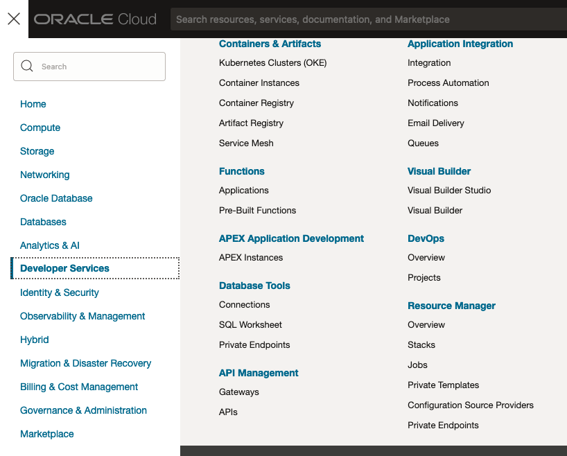
You’ll need to go to the Resource Manager page. This can be found under the menu by going to the Developer Services and then selecting Resource Manager.
First, you’ll need to go to the Resource Manager page. This can be found under the menu by going to the Developer Services and then selecting Resource Manager.
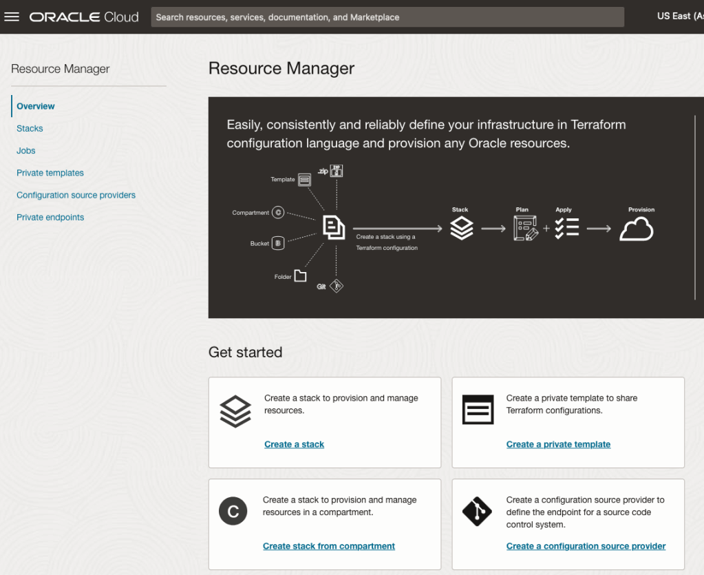
Located just under the main banner image you’ll see a section labelled ‘Create a stack’. Click on this link.
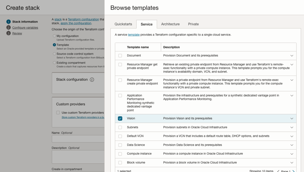
In the Create stack screen select Template from the radio group at the top of the page. Then in the Browse template pop-up screen, select the Service tab (across the top) and locate Vision. Once selected click the Select Template button.
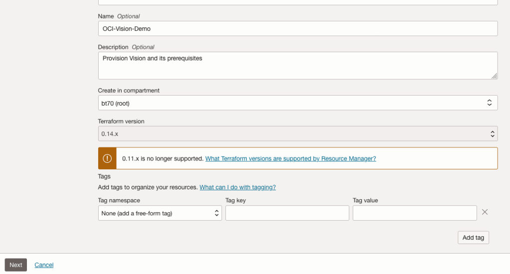
The page will load the necessary configuration. The only other thing you need to change on this page is the Name of the Service. Make it meaningful for you and your project. Click the Next button to continue to the next screen.
The top section relates to IAM Group name and policy configuration. You take the defaults or if you have specific groups already configured you can change it to it.
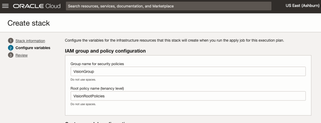
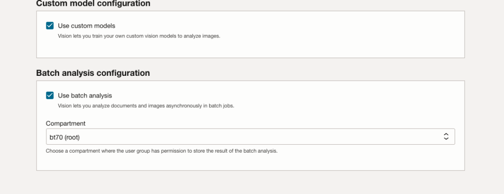
Most people will want to create their own customer models, as the supplied pre-built models are a bit basic. To enable Custom Built models, just tick the checkbox in the Custom Model Configuration section.
The second checkbox enables the batch processing of documents/images. If you check this box, you’ll need to specify the compartment you want the workload to be assigned to. Then click the Next button.
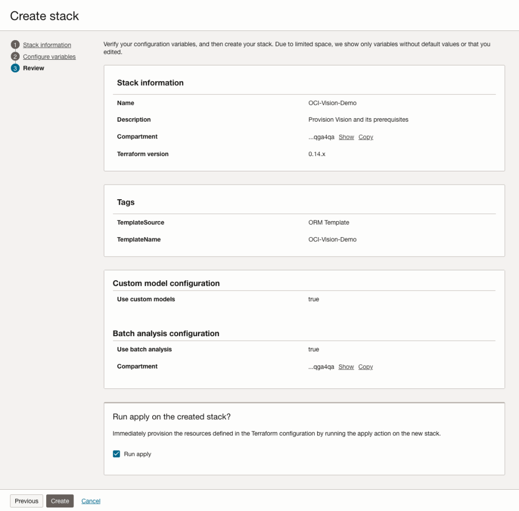
The final part displays a verification page of what was selected in the previous steps.
When ready click on the Run Apply check box and then click on the Create button.
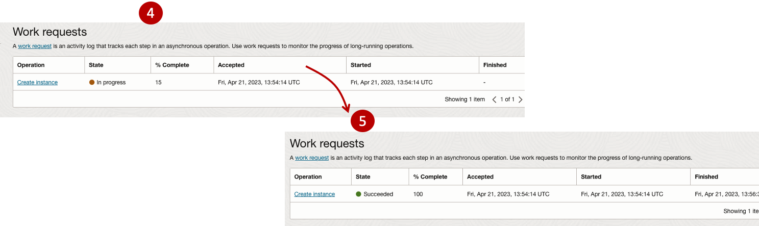
It can take anything from a few seconds or a couple of minutes for the scripts to run.
When completed you’ll a Green box at the top of the screen and the message ‘SUCCEEDED’ under it.

Machine Learning App Migration to Oracle Cloud VM
Over the past few years, I’ve been developing a Stock Market prediction algorithm and made some critical refinements to it earlier this year. As with all analytics, data science, machine learning and AI projects, testing is vital to ensure its performance, accuracy and sustainability. Taking such a project out of a lab environment and putting it into a production setting introduces all sorts of different challenges. Some of these challenges include being able to self-manage its own process, logging, traceability, error and event management, etc. Automation is key and implementing all of these extra requirements tasks way more code and time than developing the actual algorithm. Typically, the machine learning and algorithms code only accounts for less than five percent of the actual code, and in some cases, it can be less than one percent!
I’ve come to the stage of deploying my App to a production-type environment, as I’ve been running it from my laptop and then a desktop for over a year now. It’s now 100% self-managing so it’s time to deploy. The environment I’ve chosen is using one of the Virtual Machines (VM) available on the Oracle Free Tier. This means it won’t cost me a cent (dollar or more) to run my App 24×7.
My App has three different components which use a core underlying machine learning predictions engine. Each is focused on a different set of stock markets. These marks operate in the different timezone of US markets, European Markets and Asian Markets. Each will run on a slightly different schedule than the rest.
The steps outlined below take you through what I had to do to get my App up and running the VM (Oracle Free Tier). It took about 20 minutes to complete everything
The first thing you need to do is create a ssh key file. There are a number of ways of doing this and the following is an example.
ssh-keygen -t rsa -N "" -b 2048 -C "myOracleCloudkey" -f myOracleCloudkey
This key file will be used during the creation of the VM and for logging into the VM.
Log into your Oracle Cloud account and you’ll find the Create Instances Compute i.e. create a virtual machine/

Complete the Create Instance form and upload the ssh file you created earlier. Then click the Create button. This assumes you have networking already created.

It will take a minute or two for the VM to be created and you can monitor the progress.
After it has been created you need to click on the start button to start the VM.
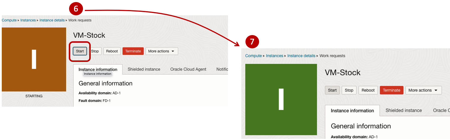
After it has started you can now log into the VM from a terminal window, using the public IP address
ssh -i myOracleCloudKey opc@xxx.xxx.xxx.xxxAfter you’ve logged into the VM it’s a good idea to run an update.
[opc@vm-stocks ~]$ sudo yum -y update
Last metadata expiration check: 0:13:53 ago on Fri 21 Apr 2023 14:39:59 GMT.
Dependencies resolved.
========================================================================================================================
 Package                         Arch       Version                                          Repository            Size
========================================================================================================================
Installing:
 kernel-uek                      aarch64    5.15.0-100.96.32.el8uek                          ol8_UEKR7            1.4 M
 kernel-uek-core                 aarch64    5.15.0-100.96.32.el8uek                          ol8_UEKR7             47 M
 kernel-uek-devel                aarch64    5.15.0-100.96.32.el8uek                          ol8_UEKR7             19 M
 kernel-uek-modules              aarch64    5.15.0-100.96.32.el8uek                          ol8_UEKR7             59 M
Upgrading:
 NetworkManager                  aarch64    1:1.40.0-6.0.1.el8_7                             ol8_baseos_latest    2.1 M
 NetworkManager-config-server    noarch     1:1.40.0-6.0.1.el8_7                             ol8_baseos_latest    141 k
 NetworkManager-libnm            aarch64    1:1.40.0-6.0.1.el8_7                             ol8_baseos_latest    1.9 M
 NetworkManager-team             aarch64    1:1.40.0-6.0.1.el8_7                             ol8_baseos_latest    156 k
 NetworkManager-tui              aarch64    1:1.40.0-6.0.1.el8_7                             ol8_baseos_latest    339 k
...
...
The VM is now ready to setup and install my App. The first step is to install Python, as all my code is written in Python.
[opc@vm-stocks ~]$ sudo yum install -y python39
Last metadata expiration check: 0:20:35 ago on Fri 21 Apr 2023 14:39:59 GMT.
Dependencies resolved.
========================================================================================================================
 Package                         Architecture  Version                                        Repository           Size
========================================================================================================================
Installing:
 python39                        aarch64       3.9.13-2.module+el8.7.0+20879+a85b87b0         ol8_appstream        33 k
Installing dependencies:
 python39-libs                   aarch64       3.9.13-2.module+el8.7.0+20879+a85b87b0         ol8_appstream       8.1 M
 python39-pip-wheel              noarch        20.2.4-7.module+el8.6.0+20625+ee813db2         ol8_appstream       1.1 M
 python39-setuptools-wheel       noarch        50.3.2-4.module+el8.5.0+20364+c7fe1181         ol8_appstream       497 k
Installing weak dependencies:
 python39-pip                    noarch        20.2.4-7.module+el8.6.0+20625+ee813db2         ol8_appstream       1.9 M
 python39-setuptools             noarch        50.3.2-4.module+el8.5.0+20364+c7fe1181         ol8_appstream       871 k
Enabling module streams:
 python39                                      3.9

Transaction Summary
========================================================================================================================
Install  6 Packages

Total download size: 12 M
Installed size: 47 M
Downloading Packages:
(1/6): python39-pip-20.2.4-7.module+el8.6.0+20625+ee813db2.noarch.rpm                    23 MB/s | 1.9 MB     00:00
(2/6): python39-pip-wheel-20.2.4-7.module+el8.6.0+20625+ee813db2.noarch.rpm             5.5 MB/s | 1.1 MB     00:00
...
...
Next copy the code to the VM, setup the environment variables and create any necessary directories required for logging. The final part of this is to download the connection Wallett for the Database. I’m using the Python library oracledb, as this requires no additional setup.
Then install all the necessary Python libraries used in the code, for example, pandas, matplotlib, tabulate, seaborn, telegram, etc (this is just a subset of what I needed). For example here is the command to install pandas.
pip3.9 install pandasAfter all of that, it’s time to test the setup to make sure everything runs correctly.
The final step is to schedule the App/Code to run. Before setting the schedule just do a quick test to see what timezone the VM is running with. Run the date command and you can see what it is. In my case, the VM is running GMT which based on the current time locally, the VM was showing to be one hour off. Allowing for this adjustment and for day-light saving time, the time +/- markets openings can be set. The following example illustrates setting up crontab to run the App, Monday-Friday, between 13:00-22:00 and at 5-minute intervals. Open crontab and edit the schedule and command. The following is an example
> contab -e

*/5 13-22 * * 1-5 python3.9 /home/opc/Stocks.py >Stocks.txt
For some stock market trading apps, you might want it to run more frequently (than every 5 minutes) or less frequently depending on your strategy.
After scheduling the components for each of the Geographic Stock Market areas, the instant messaging of trades started to appear within a couple of minutes. After a little monitoring and validation checking, it was clear everything was running as expected. It was time to sit back and relax and see how this adventure unfolds.
For anyone interested, the App does automated trading with different brokers across the markets, while logging all events and trades to an Oracle Autonomous Database (Free Tier = no cost), and sends instant messages to me notifying me of the automated trades. All I have to do is Nothing, yes Nothing, only to monitor the trade notifications. I mentioned earlier the importance of testing, and with back-testing of the recent changes/improvements (as of the date of post), the App has given a minimum of 84% annual return each year for the past 15 years. Most years the return has been a lot more!
Oracle 23c Free – Developer Release
Oracle 23c if finally available, in the form of Oracle 23c FREE – Developer Release. There was lots of excitement in some parts of the IT community about this release, some of which is to do with people having to wait a while for this release, given 22c was never released due to Covid!
But some caution is needed and reining back on the excitement is needed.

Why? This release isn’t the full bells and whistles full release of 23c Database. There has been several people from Oracle emphasizing the name of this release is Oracle 23c Free – Developer Release. There are a few things to consider with this release. It isn’t a GA (General Available) Release which is due later this year (maybe). Oracle 23c Free – Developer Release is an early release to allow developers to start playing with various developer focused new features. Some people have referred to this as the 23c Beta version 2 release, and this can be seen in the DB header information. It could be viewed in a similar way as the XE releases we had previously. XE was always Free, so we now we have a rename and emphasis of this. These have been many, many organizations using the XE release to build applications. Also the the XE releases were a no cost option, or what most people would like to say, the FREE version.
For the full 23c Database release we will get even more features, but most of these will probably be larger enterprise scale scenarios.
Now it’s time you to go play with 23c Free – Developer Release. Here are some useful links
- Product Release Official Announcement
- Post by Gerald Venzi
- See link for Docker installation below
- VirtualBox Virtual Machine
- You want to do it old school – Download RPM files
- New Features Guide
I’ll be writing posts on some of the more interesting new features and I’ll add the links to those below. I’ll also add some links to post by other people:
- Docker Installation (Intel and Apple Chip)
- 23 Free Virtual Machine
- 23 Free – A Few (New Features) A few Quickies
- JSON Relational Duality – see post by Tim Hall
- more coming soon (see maintained list at https://oralytics.com/23c/)
Annual Look at Database Trends (Jan 2023)
Monitoring trends in the popularity and usage of different Database vendors can be a interesting exercise. The marketing teams from each vendor do an excellent job of promoting their Database, along with the sales teams, developer advocates, and the user communities. Some of these are more active than others and it varies across the Database market on what their choice is for promoting their products. One of the problems with these various types of marketing, is how can be believe what they are saying about how “awesome” their Database is, and then there are some who actively talk about how “rubbish” (or saying something similar) other Databases area. I do wonder how this really works for these people and vendors when to go negative about their competitors. A few months ago I wrote about “What does Legacy Really Mean?“. That post was prompted by someone from one Database Vendor calling their main competitor Database a legacy product. They are just name calling withing providing any proof or evidence to support what they are saying.
Getting back to the topic of this post, I’ve gathered some data and obtained some league tables from some sites. These will help to have a closer look at what is really happening in the Database market throughout 2022. Two popular sites who constantly monitor the wider internet and judge how popular Databases area globally. These sites are DB-Engines and TOPDB Top Database index. These are well know and are frequently cited. Both of these sites give some details of how they calculate their scores, with one focused mainly on how common the Database appears in searches across different search engines, while the other one, in addition to search engine results/searches, also looks across different websites, discussion forms, social media, job vacancies, etc.
The first image below is a comparison of the league tables from DB-Engines taken in January 2022 and January 2023. I’ve divided this image into three sections/boxes. Overall for the first 10 places, not a lot has changed. The ranking scores have moved slightly in most cases but not enough to change their position in the rank. Even with a change of score by 30+ points is a very small change and doesn’t really indicate any great change in the score as these scores are ranked in a manner where, “when system A has twice as large a value in the DB-Engines Ranking as system B, then it is twice as popular when averaged over the individual evaluation criteria“. Using this explanation, Oracle would be twice as popular when compared to PostgreSQL. This is similar across 2022 and 2023.

Next we’ll look a ranking from TOPDB Top Database index. The image below compares January 2022 and January 2023. TOPDB uses a different search space and calculation for its calculation. The rankings from TOPDB do show some changes in the ranks and these are different to those from DB-Engines. Here we see the top three ranks remain the same with some small percentage changes, and nothing to get excited about. In the second box covering ranks 4-7 we do some changes with PostgreSQL improving by two position and MongoDB. These changes do seem to reflect what I’ve been seeing in the marketplace with MongoDB being replaced by PostgreSQL and MySQL, with this multi-model architecture where you can have relational, document, and other data models in the one Database. It’s important to note Oracle and SQL Server also support this. Over the past couple of years there has been a growing awareness of and benefits of having relation and document (and others) data models in the one database. This approach makes sense both for developer productivity, and for data storage and management.

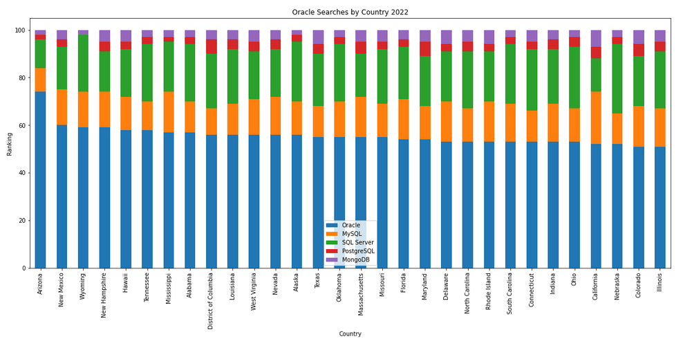
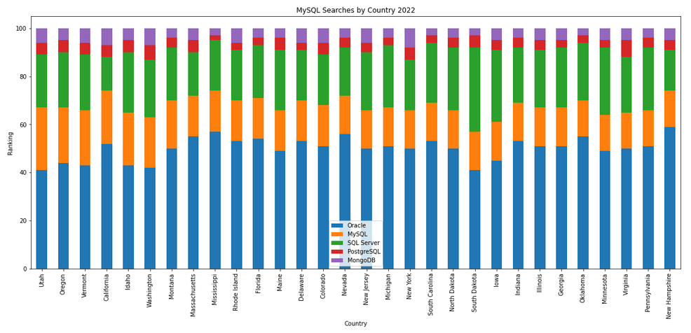
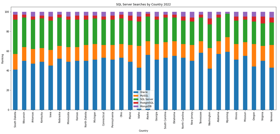
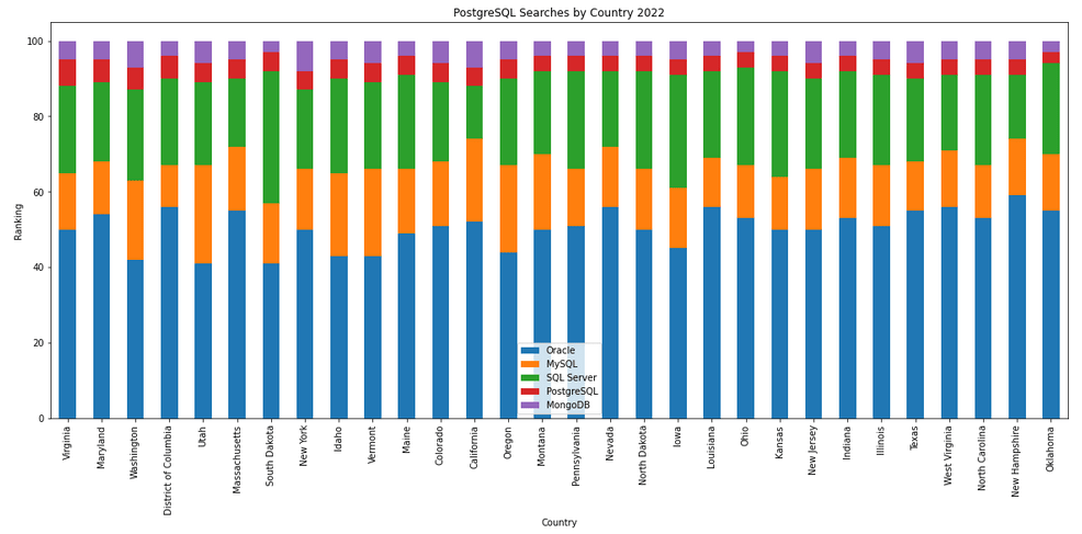
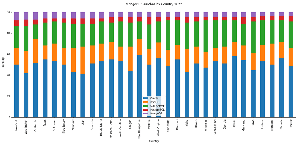
The next gallery of images is based on some Python code I’ve written to look a little bit closer at the top five Databases. In this case these are Oracle, MySQL, SQL Server, PostgreSQL and MongoDB. This gallery plots a bar chart for each Database for their top 15 Counties, and compares them with the other four Databases. The results are interesting and we can see some geographic aspects to the popularity of the Databases.
Number of rows in each Table – Various Databases
A possible common task developers perform is to find out how many records exists in every table in a schema. In the examples below I’ll show examples for the current schema of the developer, but these can be expanded easily to include tables in other schemas or for all schemas across a database.
These example include the different ways of determining this information across the main databases including Oracle, MySQL, Postgres, SQL Server and Snowflake.
A little warning before using these queries. They may or may not give the true accurate number of records in the tables. These examples illustrate extracting the number of records from the data dictionaries of the databases. This is dependent on background processes being run to gather this information. These background processes run from time to time, anything from a few minutes to many tens of minutes. So, these results are good indication of the number of records in each table.
Oracle
SELECT table_name, num_rows
FROM user_tables
ORDER BY num_rows DESC;
or
SELECT table_name,
       to_number(
          extractvalue(xmltype(
             dbms_xmlgen.getxml('select count(*) c from '||table_name))
                ,'/ROWSET/ROW/C')) tab_count
FROM   user_tables
ORDER BY tab_count desc;
Using PL/SQL we can do something like the following.
DECLARE
   val NUMBER;
BEGIN
   FOR i IN (SELECT table_name FROM user_tables ORDER BY table_name desc) LOOP
      EXECUTE IMMEDIATE 'SELECT count(*) FROM '|| i.table_name INTO val;
      DBMS_OUTPUT.PUT_LINE(i.table_name||' -> '|| val );
   END LOOP;
END;
MySQL
SELECT table_name, table_rows
FROM INFORMATION_SCHEMA.TABLES
WHERE table_type = 'BASE TABLE'
AND  TABLE_SCHEMA = current_user();
Using Common Table Expressions (CTE), using WITH clause
WITH table_list AS (
SELECT
    table_name
  FROM information_schema.tables
  WHERE table_schema = current_user()
  AND
        table_type = 'BASE TABLE'
)
SELECT CONCAT(
            GROUP_CONCAT(CONCAT("SELECT '",table_name,"' table_name,COUNT(*) rows FROM ",table_name) SEPARATOR " UNION "),
            ' ORDER BY table_name'
        )
INTO @sql
FROM table_list;
Postgres
select relname as table_name, n_live_tup as num_rows from pg_stat_user_tables;
An alternative is
select n.nspname as table_schema,
       c.relname as table_name,
       c.reltuples as rows
from pg_class c
join pg_namespace n on n.oid = c.relnamespace
where c.relkind = 'r'
      and n.nspname = current_user
order by c.reltuples desc;
SQL Server
SELECT tab.name,
       sum(par.rows)
FROM   sys.tables tab INNER JOIN sys.partitions par
          ON tab.object_id = par.object_id
WHERE  schema_name(tab.schema_id) = current_user
Snowflake
SELECT t.table_schema, t.table_name, t.row_count
FROM   information_schema.tables t
WHERE  t.table_type = 'BASE TABLE'
AND    t.table_schema = current_user
order by t.row_count desc;
The examples give above are some of the ways to obtain this information. As with most things, there can be multiple ways of doing it, and most people will have their preferred one which is based on their background and preferences.
As you can see from the code given above they are all very similar, with similar syntax, etc. The only thing different is the name of the data dictionary table/view containing the information needed. Yes, knowing what data dictionary views to query can be a little challenging as you switch between databases.
AUTO_PARTITION – Inspecting & Implementing Recommendations
In a previous blog post I gave an overview of the DBMS_AUTO_PARTITION package in Oracle Autonomous Database. This looked at how you can get started and to setup Auto Partitioning and to allow it to automatically implement partitioning.
This might not be something the DBAs will want to happen for lots of different reasons. An alternative is to use DBMS_AUTO_PARTITION to make recommendations for tables where partitioning will have a performance improvement. The DBA can inspect these recommendations and decide which of these to implement.
In the previous post we set the CONFIGURE function to be ‘IMPLEMENT’. We need to change that to report the recommendations.
exec dbms_auto_partition.configure('AUTO_PARTITION_MODE','REPORT ONLY');Just remember, tables will only be considered by AUTO_PARTITION as outlined in my previous post.
Next we can ask for recommendations using the RECOMMEND_PARTITION_METHOD function.
exec  dbms_auto_partition.recommend_partition_method(
   table_owner => 'WHISKEY',
   table_name => 'DIRECTIONS',
   report_type => 'TEXT',
   report_section => 'ALL',
   report_level => 'ALL');
The results from this are stored in DBA_AUTO_PARTITION_RECOMMENDATIONS, which you can query to view the recommendations.
select recommendation_id, partition_method, partition_key
from dba_auto_partition_recommendations;
RECOMMENDATION_ID PARTITION_METHOD PARTITION_KEY
-------------------------------- ------------------------------------------------------------------------------------------------------------- --------------
D28FC3CF09DF1E1DE053D010000ABEA6 Method: LIST(SYS_OP_INTERVAL_HIGH_BOUND("D", INTERVAL '2' MONTH, TIMESTAMP '2019-08-10 00:00:00')) AUTOMATIC D
To apply the recommendation pass the RECOMMENDATION_KEY value to the APPLY_RECOMMENDATION function.
exec dbms_auto_partition.apply_recommendation('D28FC3CF09DF1E1DE053D010000ABEA6');It might takes some minutes for the partitioned table to become available. During this time the original table will remain available as the change will be implemented using a ALTER TABLE MODIFY PARTITION ONLINE command.
Two other functions include REPORT_ACTIVITY and REPORT_LAST_ACTIVITY. These can be used to export a detailed report on the recommendations in text or HTML form. It is probably a good idea to create and download these for your change records.
spool autoPartitionFinding.html
select dbms_auto_partition.report_last_activity(type=>'HTML') from dual;
exit;AUTO_PARTITION – Basic setup
Partitioning is an effective way to improve performance of SQL queries on large volumes of data in a database table. But only so, if a bit of care and attention is taken by both the DBA and Developer (or someone with both of these roles). Care is needed on the database side to ensure the correct partitioning method is deployed and the management of these partitions, as some partitioning methods can create a significantly large number of partitions, which in turn can affect the management of these and possibly performance too, which is not what you want. Care is also needed from the developer side to ensure their code is written in a way that utilises the partitioning method deployed. If doesn’t then you may not see much improvement in performance of your queries, and somethings things can run slower. Which not one wants!
With the Oracle Autonomous Database we have the expectation it will ‘manage’ a lot of the performance features behind the scenes without the need for the DBA and Developing getting involved (‘Autonomous’). This is kind of true up to a point, as the serverless approach can work up to a point. Sometimes a little human input is needed to give a guiding hand to the Autonomous engine to help/guide it towards what data needs particular focus.
In this (blog post) case we will have a look at DBMS_AUTO_PARTITION and how you can do a basic setup, config and enablement. I’ll have another post that will look at the recommendation feature of DBMS_AUTO_PARTITION. Just a quick reminder, DBMS_AUTO_PARTITION is for the Oracle Autonomous Database (ADB) (on the Cloud). You’ll need to run the following as ADMIN user.
The first step is to enable auto partitioning on the ADB using the CONFIGURE function. This function can have three parameters:
- IMPLEMENT : generates a report and implements the recommended partitioning method. (Autonomous!)
- REPORT_ONLY : {default} reports recommendations for partitioning on tables
- OFF : Turns off auto partitioning (reporting and implementing)
For example, to enable auto partitioning and to automatically implement the recommended partitioning method.
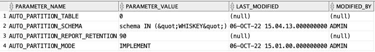
exec DBMS_AUTO_PARTITION.CONFIGURE('AUTO_PARTITION_MODE', 'IMPLEMENT');The changes can be inspected in the DBA_AUTO_PARTITION_CONFIG view.
SELECT * FROM DBA_AUTO_PARTITION_CONFIG;When you look at the listed from the above select we can see IMPLEMENT is enabled

The next step with using DBMS_AUTO_PARTITION is to tell the ADB what schemas and/or tables to include for auto partitioning. This first example shows how to turn on auto partitioning for a particular schema, and to allow the auto partitioning (engine) to determine what is needed and to just go and implement that it thinks is the best partitioning methods.
exec DBMS_AUTO_PARTITION.CONFIGURE(
   parameter_name => 'AUTO_PARTITION_SCHEMA',
   parameter_value => 'WHISKEY',
   ALLOW => TRUE);
If you query the DBA view again we now get.
We have not enabled a schema (called WHISKEY) to be included as part of the auto partitioning engine.
Auto Partitioning may not do anything for a little while, with some reports suggesting to wait for 15 minutes for the database to pick up any changes and to make suggestions. But there are some conditions for a table needs to meet before it can be considered, this is referred to as being a ‘Candidate’. These conditions include:
- Table passes inclusion and exclusion tests specified by AUTO_PARTITION_SCHEMA and AUTO_PARTITION_TABLE configuration parameters.
- Table exists and has up-to-date statistics.
- Table is at least 64 GB.
- Table has 5 or more queries in the SQL tuning set that scanned the table.
- Table does not contain a LONG data type column.
- Table is not manually partitioned.
- Table is not an external table, an internal/external hybrid table, a temporary table, an index-organized table, or a clustered table.
- Table does not have a domain index or bitmap join index.
- Table is not an advance queuing, materialized view, or flashback archive storage table.
- Table does not have nested tables, or certain other object features.
If you find Auto Partitioning isn’t partitioning your tables (i.e. not a valid Candidate) it could be because the table isn’t meeting the above list of conditions.
This can be verified using the VALIDATE_CANDIDATE_TABLE function.
select DBMS_AUTO_PARTITION.VALIDATE_CANDIDATE_TABLE(
   table_owner => 'WHISKEY',
   table_name => 'DIRECTIONS')
from dual;
If the table has met the above list of conditions, the above query will return ‘VALID’, otherwise one or more of the above conditions have not been met, and the query will return ‘INVALID:’ followed by one or more reasons
Check out my other blog post on using the AUTO_PARTITION to explore it’s recommendations and how to implement.
OML4R available on ADB
Oracle Machine Learning for R (OML4R) is available on Oracle Autonomous Database. Finally. After waiting for way, way too long we can now run R code in the Autonomous Database (in the Cloud). It’s based on using Oracle R Distribution 4.0.5 (which is based on R 4.0.5). This product was previously called Oracle R Enterprise, which I was a fan of many few years ago, so much so I wrote a book about it.
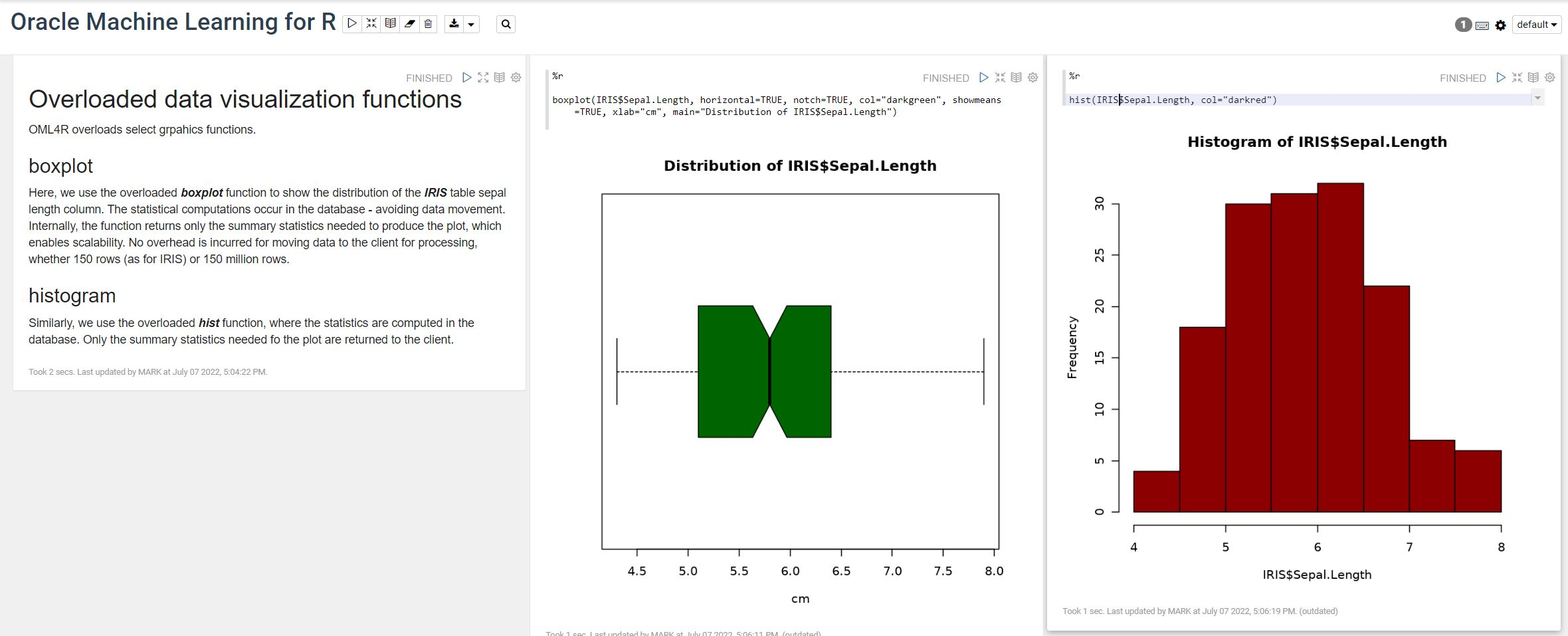
OML4R comes with all (or most) of the benefits of Oracle R Enterprise, whereby you can connect to, in this case an Oracle Autonomous Database (in the Cloud), allowing data scientists work with R code and manipulate data in the database instead of in their local environment. Embed R code in the database and enable other database users (and applications) to call this R code. Although with OML4R on ADB (in the Cloud) does come with some limitations and restrictions, which will put people/customers off from using it.
Waiting for OML4R reminds me of Eurovision Song Contest winning song by Johnny Logan titled,
I’ve been waiting such a long time
Looking out for you
But you’re not here
What’s another year
It has taken Oracle way, way too long to migrate OML4R to ADB. They’ve probably just made it available because one or two customers needed/asked it.
As the lyrics from Johnny Logan says (changing I’ve to We’ve), We’ve been waiting such a long time, most customers have moved to other languages, tools and other cloud data science platforms for their data science work. The market has moved on, many years ago.
Hopefully over the next few months, and with Oracle 23c Database, we might see some innovation, or maybe their data science and AI focus lies elsewhere within Oracle development teams.

You must be logged in to post a comment.