
Oracle
Exploring Apache Iceberg – Part 4 – Parquet Files with Oracle Autonomous Database
In this post I’ll walk through the steps needed to setup and use Parquet files with an Oracle Autonomous Database and with the parquet files stored in Oracle Cloud. In my previous post, did something similar but for an on-premises Oracle Database.
Generally the setup is very similar except for two particular parts where we need to load the parquet files into a bucket on Oracle cloud (OCI) and the secondly we need some additional configuration in the Database to be able to access those files in an OCI bucket.
Create Bucket and Upload files
In OCI Storage section of OCI, create a new bucket (Parquet-files) and upload the parquet files. You can automate this step with a simple piece of Python code.
Create Credential
Log into the schema you are going to use to create the external table. You’ll need to generate an authentication token.
BEGIN DBMS_CLOUD.CREATE_CREDENTIAL( credential_name => 'PARQUET_FILES_CRED', username => '<your cloud username>', password => '<generated auth token>' );END;
Create the External table
We can now create the external table pointing to the parquet files in the OCI bucket.
BEGIN DBMS_CLOUD.CREATE_EXTERNAL_TABLE( table_name => 'PARQUET_FILES_EXT', credential_name => 'PARQUET_FILES_CRED', file_uri_list => 'https://objectstorage.us-ashburn-1.oraclecloud.com/n/<namespace>/b/Parquet-Files/o/*.parquet', format => JSON_OBJECT( 'type' VALUE 'parquet', 'schema' VALUE 'first', 'blankasnull' VALUE 'true', 'trimspaces' VALUE 'lrtrim' ) );END;/
Query the Parquet Files
We can now query the parquet files.
SELECT region, product, SUM(amount) AS total_salesFROM parquet_files_extGROUP BY regionORDER BY total_sales DESC;
Exploring Apache Iceberg – Part 3 – Parquet Files with Oracle Database
In this post I’ll explore how you can included data in Parquet files in an Oracle Database. This is a little sideways post from my previous posts on Apache Iceberg, as it will only look at using Parquet files, which are a core part of Iceberg tables, but is missing the meta-data layer that Iceberg tables gives.
The previous two posts on Apache Iceberg looked at using PyIceberg Python package to create and to explore the various feature of Iceberg and it’s effects on the data, files and meta-data. Part-1, Part-2.
We can include Parquet files in an Oracle Database by creating an External Table based on those files. Let’s walk through an example. The following example will for an “On-Premises” Database. I’ll have an example later in this post if you are using an Oracle Autonomous Database on Oracle Cloud.
Log into the Database as SYSTEM user, create a directory option to point to the location of the files on the operating system, and then grant privileges to the schama that needs to read that data.
CREATE OR REPLACE DIRECTORY parquet_dir AS '/data/log/parquet';GRANT READ, WRITE ON DIRECTORY parquet_dir TO parquet_user;
It is assumed the directory ‘/data/log/parquet‘ exists and has some parquet files in it.
Connect the schama “parquet_user” and create an External Table that points to the parquet files in the directory
CREATE TABLE parquet_sales_data ( sale_id NUMBER, sale_date DATE, product_id NUMBER, amount NUMBER(10,2), region VARCHAR2(50))ORGANIZATION EXTERNAL ( TYPE ORACLE_BIGDATA DEFAULT DIRECTORY parquet_dir ACCESS PARAMETERS ( com.oracle.bigdata.fileformat = PARQUET ) LOCATION ('sales_*.parquet'))REJECT LIMIT UNLIMITED;
We can not query the parquey data just like any other data in a table.
SELECT region, product, SUM(amount) AS total_salesFROM sales_externalGROUP BY regionORDER BY total_sales DESC;
Care is needed to ensure column name and datatypes match between the table and the parquet file.
If our parquet files are partitioned into directories for different time periods, we can create a Partitioned External Table to handle that data, and we it we get the benefits of partition pruning, etc and better response times.
CREATE TABLE parquet_sales_data ( sale_id NUMBER, sale_date DATE, product_id NUMBER, amount NUMBER(10,2), region VARCHAR2(50))ORGANIZATION EXTERNAL PARALLEL 4 ( TYPE ORACLE_BIGDATA DEFAULT DIRECTORY parquet_dir ACCESS PARAMETERS ( com.oracle.bigdata.fileformat = PARQUET )PARTITION BY LIST (region) ( PARTITION p_emea VALUES ('EMEA') LOCATION (emea_dir:'*.parquet'), PARTITION p_apac VALUES ('APAC') LOCATION (apac_dir:''*.parquet'), PARTITION p_amer VALUES ('AMER') LOCATION (amer_dir:'*.parquet'))REJECT LIMIT UNLIMITED;
For this example, I needed to connect as SYSTEM and create the extra directories to point to the additional directories used. I also added PARALLEL 4 to the table to help speed things up a little more.
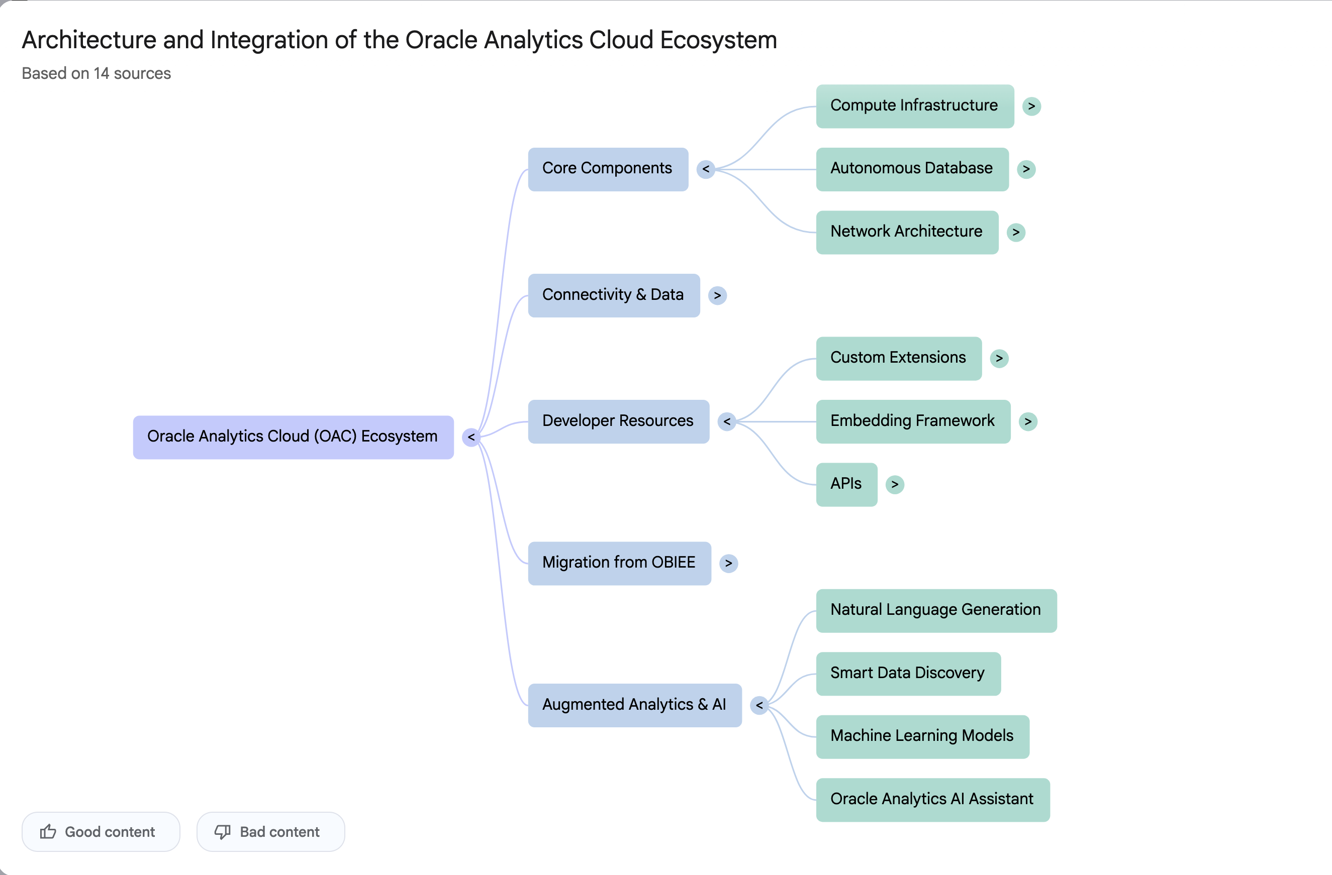
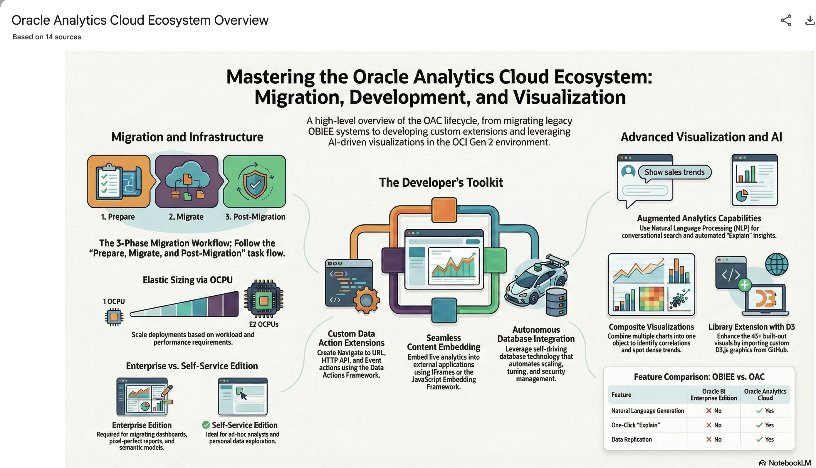
Using NotebookLM to help with understanding Oracle Analytics Cloud or any other product
Over the past few months, we’ve seen a plethora of new LLM related products/agents being released. One such one is NotebookLM from Google. The offical description say “NotebookLM is an AI-powered research and note-taking tool from Google Labs that allows users to ground a large language model (like Gemini) in their own documents, such as PDFs, Google Docs, website URLs, or audio, acting as a personal, intelligent research assistant. It facilitates summarizing, analyzing, and querying information within these specific sources to create study guides, outlines, and, notably, “Audio Overviews” (podcast-style summaries)”
Let’s have a look at using NotebookLM to help with answering questions and how it can help with understanding Oracle Analytics Cloud (OAC).

Yes, you’ll need a Google account, and Yes you need to be OK with uploading your documents to NotebookLM. Make sure you are not breaking any laws (IP, GDPR, etc). It’s really easy to create your first notebook. Simply click on ‘Create new notebook’.
When the notebook opens, you can add your documents and webpages to the notebook. These can be documents in PDF, audio, text, etc to the notebook repository. Currently, there seems to be a limit of 50 documents and webpages that can be added.
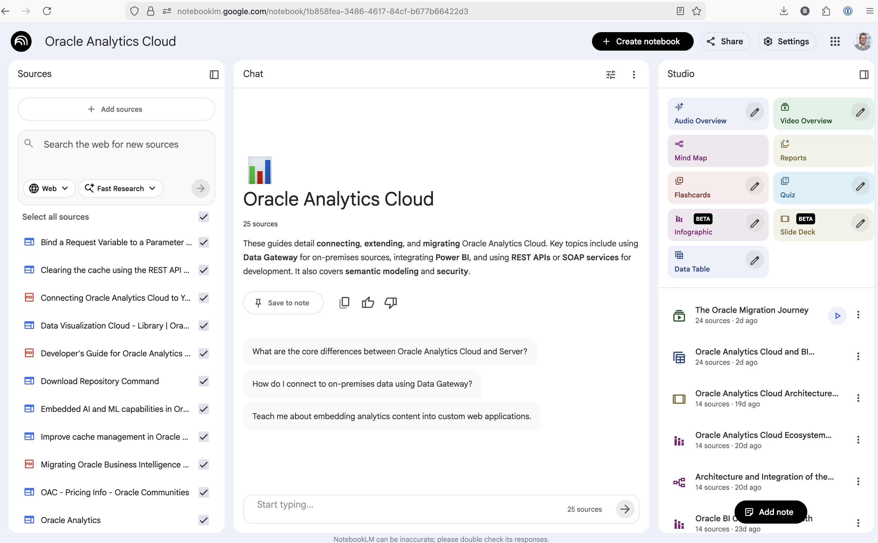
The main part of the NotebookLM provides a chatbot where you can ask questions, and the NotebookLM will search through the documents and webpages to formulate an answer. In addition to this, there are features that allow you to generate Audio Overview, Video Overview, Mind Map, Reports, Flashcards, Quiz, Infographic, Slide Deck and a Data Table.
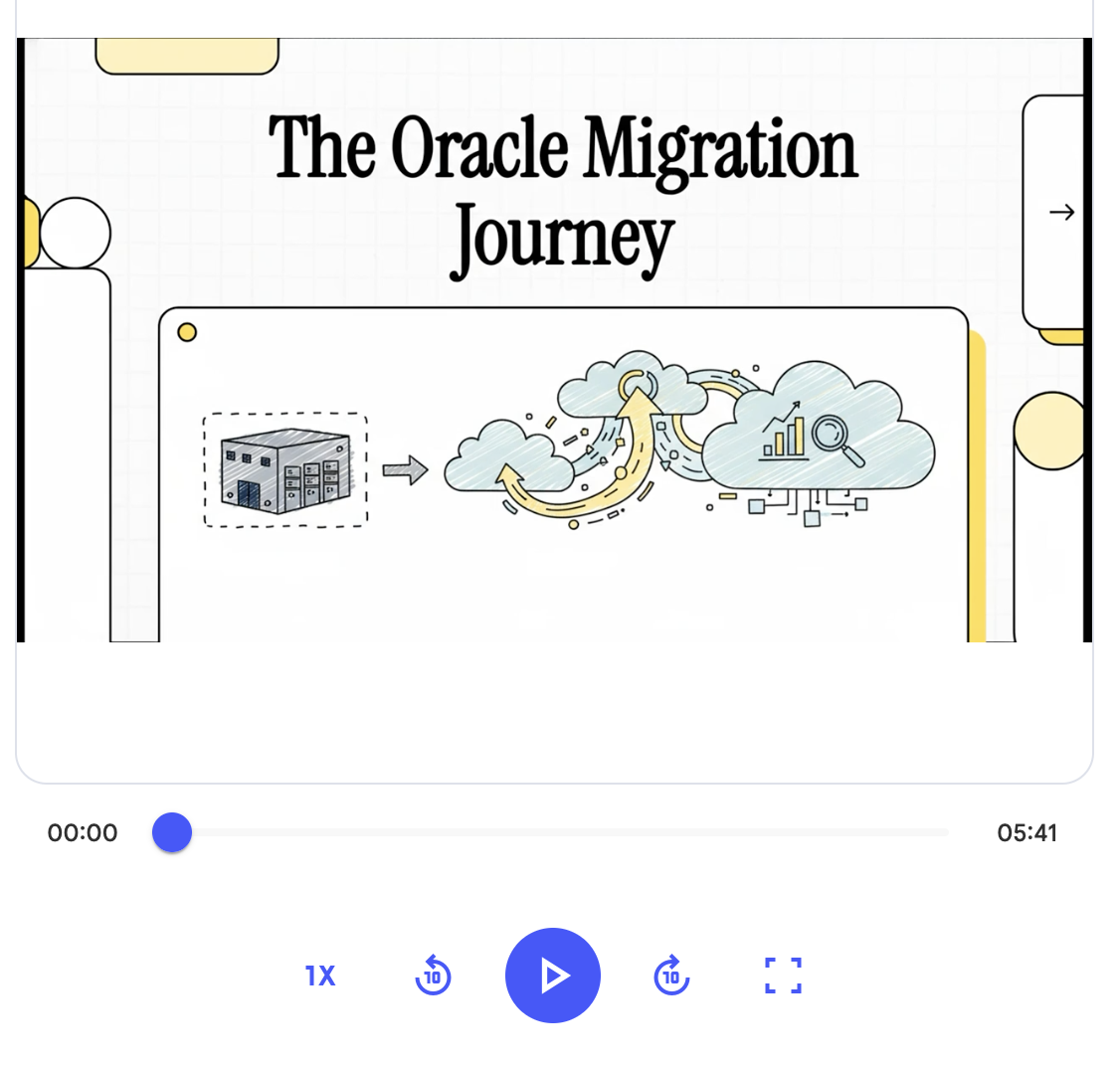
Before we look at some of these and what they have created for Oracle Analytics Cloud, there is a small warning. Some of these can take a long time to complete, that is, if they complete. I’ve had to run some of these features multiple times to get them to create. I’ve run all of the features, and the output from these can be seen on the right-hand side of the above image.
It created a 15-slide presentation on Oracle Analytics Cloud and its various features, and a five minute video on migrating OAC.
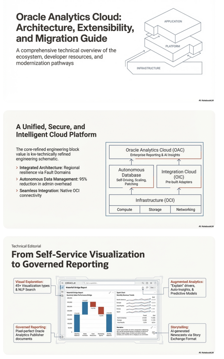
It also created a Mind-map, and an Infographic.
What a difference a Bind Variable makes
To bind or not to bind, that is the question?
Over the years, I heard and read about using Bind variables and how important they are, particularly when it comes to the efficient execution of queries. By using bind variables, the optimizer will reuse the execution plan from the cache rather than generating it each time. Recently, I had conversations about this with a couple of different groups, and they didn’t really believe me and they asked me to put together a demonstration. One group said they never heard of ‘prepared statements’, ‘bind variables’, ‘parameterised query’, etc., which was a little surprising.
The following is a subset of what I demonstrated to them to illustrate the benefits and potential benefits.
Here is a basic example of a typical scenario where we have a SQL query being constructed using concatenation.
select * from order_demo where order_id = || 'i';That statement looks simple and harmless. When we try to check the EXPLAIN plan from the optimizer we will get an error, so let’s just replace it with a number, because that’s what the query will end up being like.
select * from order_demo where order_id = 1;When we check the Explain Plan, we get the following. It looks like a good execution plan as it is using the index and then doing a ROWID lookup on the table. The developers were happy, and that’s what those recent conversations were about and what they are missing.
-------------------------------------------------------------
| Id  | Operation                   | Name         | E-Rows |
-------------------------------------------------------------
|   0 | SELECT STATEMENT            |              |        |
|   1 |  TABLE ACCESS BY INDEX ROWID| ORDER_DEMO   |      1 |
|*  2 |   INDEX UNIQUE SCAN         | SYS_C0014610 |      1 |
-------------------------------------------------------------
The missing part in their understanding was what happens every time they run their query. The Explain Plan looks good, so what’s the problem? The problem lies with the Optimizer evaluating the execution plan every time the query is issued. But the developers came back with the idea that this won’t happen because the execution plan is cached and will be reused. The problem with this is how we can test this, and what is the alternative, in this case, using bind variables (which was my suggestion).
Let’s setup a simple test to see what happens. Here is a simple piece of PL/SQL code which will look 100K times to retrieve just one row. This is very similar to what they were running.
DECLARE
   start_time TIMESTAMP;
   end_time   TIMESTAMP;
BEGIN
   start_time := systimestamp;
   dbms_output.put_line('Start time : ' || to_char(start_time,'HH24:MI:SS:FF4'));
   --
   for i in 1 .. 100000 loop
      execute immediate 'select * from order_demo where order_id = '||i;
   end loop;
   --
   end_time := systimestamp;
   dbms_output.put_line('End time : ' || to_char(end_time,'HH24:MI:SS:FF4'));
END;
/
When we run this test against a 23.7 Oracle Database running in a VM on my laptop, this completes in little over 2 minutes
Start time : 16:26:04:5527
End time : 16:28:13:4820


PL/SQL procedure successfully completed.

Elapsed: 00:02:09.158
The developers seemed happy with that time! Ok, but let’s test it using bind variables and see if it’s any different. There are a few different ways of setting up bind variables. The PL/SQL code below is one example.
DECLARE
   order_rec  ORDER_DEMO%rowtype;
   start_time TIMESTAMP;
   end_time   TIMESTAMP;
BEGIN
   start_time := systimestamp;
   dbms_output.put_line('Start time : ' || to_char(start_time,'HH24:MI:SS:FF9'));
   --
   for i in 1 .. 100000 loop
   execute immediate 'select * from order_demo where order_id = :1' using i;
	end loop;
	--
    end_time := systimestamp;
    dbms_output.put_line('End time : ' || to_char(end_time,'HH24:MI:SS:FF9'));
END;
/
Start time : 16:31:39:162619000
End time : 16:31:40:479301000


PL/SQL procedure successfully completed.

Elapsed: 00:00:01.363
This just took a little over one second to complete. Let me say that again, a little over one second to complete. We went from taking just over two minutes to run, down to just over one second to run.
The developers were a little surprised or more correctly, were a little shocked. But they then said the problem with that demonstration is that it is running directly in the Database. It will be different running it in Python across the network.
Ok, let me set up the same/similar demonstration using Python. The image below show some back Python code to connect to the database, list the tables in the schema and to create the test table for our demonstration

The first demonstration is to measure the timing for 100K records using the concatenation approach. I
# Demo - The SLOW way - concat values
#print start-time
print('Start time: ' + datetime.now().strftime("%H:%M:%S:%f"))

# only loop 10,000 instead of 100,000 - impact of network latency
for i in range(1, 100000):
    cursor.execute("select * from order_demo where order_id = " + str(i))

#print end-time
print('End time: ' + datetime.now().strftime("%H:%M:%S:%f"))
----------
Start time: 16:45:29:523020
End time: 16:49:15:610094
This took just under four minutes to complete. With PL/SQL it took approx two minutes. The extrat time is due to the back and forth nature of the client-server communications between the Python code and the Database. The developers were a little unhappen with this result.
The next step for the demonstrataion was to use bind variables. As with most languages there are a number of different ways to write and format these. Below is one example, but some of the others were also tried and give the same timing.
#Bind variables example - by name

#print start-time
print('Start time: ' + datetime.now().strftime("%H:%M:%S:%f"))

for i in range(1, 100000):
    cursor.execute("select * from order_demo where order_id = :order_num", order_num=i )

#print end-time
print('End time: ' + datetime.now().strftime("%H:%M:%S:%f"))
----------
Start time: 16:53:00:479468
End time: 16:54:14:197552
This took 1 minute 14 seconds. [Read that sentence again]. Compared to approx four minutes, and yes the other bind variable options has similar timing.
To answer the quote at the top of this post, “To bind or not to bind, that is the question?”, the answer is using Bind Variables, Prepared Statements, Parameterised Query, etc will make you queries and applications run a lot quicker. The optimizer will see the structure of the query, will see the parameterised parts of it, will see the execution plan already exists in the cache and will use it instead of generating the execution plan again. Thereby saving time for frequently executed queries which might just have a different value for one or two parts of a WHERE clause.
python-oracledb driver version 3 – load data into pandas df
The Python Oracle driver had a new release recently (version 3) and with it comes a new way to load data from a Table into a Pandas dataframe. This can now be done using the pyarrow library. Here’s an example:
import oracledb ora
import pyarrow py
import pandas

#create a connection to the database
con = ora.connect( <enter your connection details> )

query = "select cust_id, cust_first_name, cust_last_name, cust_city from customers"

#get Oracle DF and set array size - care is needed for setting this
ora_df = con.fetch_df_all(statement=query, arraysize=2000)

#run query and return into Pandas Dataframe
#  using pyarrow and the to_pandas() function
df = py.Table.from_arrays(ora_df.column_arrays(), names=ora_df.columns()).to_pandas()

print(df.columns)
Once you get used to the syntax it is a simpler way to get the data into dataframe.
Vector Databases – Part 2
In this post on Vector Databases, I’ll look at the main components:
- Vector Embedding Models. What they do and what they create.
- Vectors. What they represent, and why they have different sizes.
- Vector Search. An overview of what a Vector Search will do. A more detailed version of this is in a separate post.
- Vector Search Process. It’s a multi-step process and some care is needed.

Vector Embedding Models
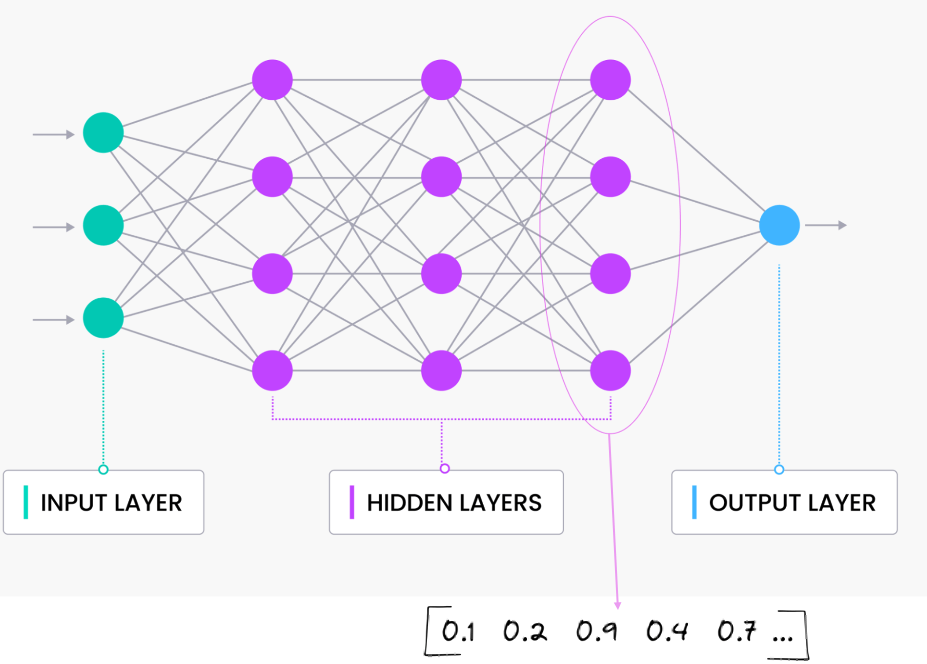
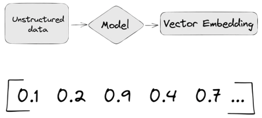
A vector embedding model is a type of machine learning model that transforms data into vectors (embeddings) in a high-dimensional space. These embeddings capture the semantic or contextual relationships between the data points, making them useful for tasks such as similarity search, clustering, and classification.
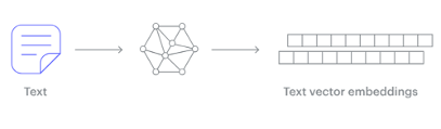
Embedding models are trained to convert the input data point (text, video, image, etc) into a vector (a series of numeric values). The model aims to identify semantic similarity with the input and map these to N-dimensional space. For example, the words “car” and “vehicle” have very different spelling but are semantically similar. The embedding model should map this to have similar vectors. Similarly with documents. The embedding model will map the documents to be able to group similar documents together (in N-dimensional space).
An embedding model is typically a Neural Network (NN) model. There are many different embedding models available from various vendor such as OpenAI, Cohere, etc., or you can build your own. Some models are open source and some are available for a fee. Typically, the output from the embedding model (the Vector) come from the last layer of the neural network
Vectors
A Vector is a sequence of numbers, called dimensions, used to capture the important “features” or “characteristics” of a piece of data. A vector is a mathematical object that has both magnitude (length) and direction. In the context of mathematics and physics, a vector is typically represented as an arrow pointing from one point to another in space, or as a list of numbers (coordinates) that define its position in a particular space.
Different Embedding Models create different numbers of Dimensions. Size is important with vectors as the greater the number number of dimensions the larger the Vector. The larger the number of dimensions the better the semantic similarity matches will be. As Vector size increases, so does space required to store them (not really a problem for Databases, but at Big Data scale it can be a challenge)
As vector size increases so does the Index space, and correspondingly search time can increase as the number of calculations for Distance Measure increases. There are various Vector indexes available to help with this (see my post covering this topic)
Basically, a vector is an array of numbers, where each number represents a dimension. It is easy for us to comprehend and visualise 2 dimensions. Here is an example of using 2 dimensions to represent different types of vehicles. The vectors give us a way to map or chart the data.
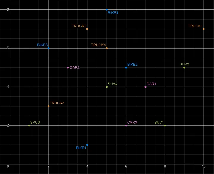
Here is SQL code for this data. I’ll come back to this data in the section on Vector Search.
INSERT INTO PARKING_LOT VALUES('CAR1','[7,4]');
INSERT INTO PARKING_LOT VALUES('CAR2','[3,5]');
INSERT INTO PARKING_LOT VALUES('CAR3','[6,2]');
INSERT INTO PARKING_LOT VALUES('TRUCK1','[10,7]');
INSERT INTO PARKING_LOT VALUES('TRUCK2','[4,7]');
INSERT INTO PARKING_LOT VALUES('TRUCK3','[2,3]');
INSERT INTO PARKING_LOT VALUES('TRUCK4','[5,6]');
INSERT INTO PARKING_LOT VALUES('BIKE1','[4,1]');
INSERT INTO PARKING_LOT VALUES('BIKE2','[6,5]');
INSERT INTO PARKING_LOT VALUES('BIKE3','[2,6]');
INSERT INTO PARKING_LOT VALUES('BIKE4','[5,8]');
INSERT INTO PARKING_LOT VALUES('SUV1','[8,2]');
INSERT INTO PARKING_LOT VALUES('SUV2','[9,5]');
INSERT INTO PARKING_LOT VALUES('SUV3','[1,2]');
INSERT INTO PARKING_LOT VALUES('SUV4','[5,4]');
The vectors created by the embedding models can have a different number of dimensions. Common Dimension Sizes are:
- 100-Dimensional: Often used in older or simpler models like some configurations of Word2Vec and GloVe. Suitable for tasks where computational efficiency is a priority and the context isn’t highly complex.
- 300-Dimensional: A common choice for many word embeddings (e.g., Word2Vec, GloVe). Strikes a balance between capturing sufficient detail and computational feasibility.
- 512-Dimensional: Used in some transformer models and sentence embeddings. Offers a richer representation than 300-dimensional embeddings.
- 768-Dimensional: Standard for BERT base models and many other transformer-based models. Provides detailed and contextual embeddings suitable for complex tasks.
- 1024-Dimensional: Used in larger transformer models (e.g., GPT-2 large). Provides even more detail but requires more computational resources.
Many of the newer embedding models have >3000 dimensions!
- Cohere’s embedding model embed-english-v3.0 has 1024 dimensions.
- OpenAI’s embedding model text-embedding-3-large has 3072 dimensions.
- Hugging Face’s embedding model all-MiniLM-L6-v2 has 384 dimensions
Here is a blog post listing some of the embedding models supported by Oracle Vector Search.
Vector Search
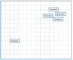
Vector search is a method of retrieving data by comparing high-dimensional vector representations (embeddings) of items rather than using traditional keyword or exact-match queries. This technique is commonly used in applications that involve similarity search, where the goal is to find items that are most similar to a given query based on their vector representations.
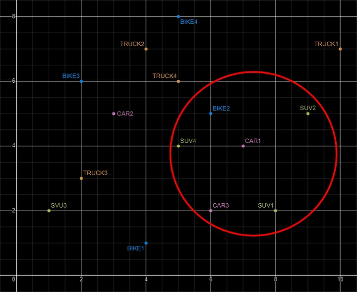
For example, using the vehicle data given above, we can easily visualise the search for similar vehicles. If we took “CAR1” as our initiating data point and wanted to know what other vehicles are similar to it. Vector Search looks at the distance between “CAR1” and all other vehicles in the 2-dimensional space.
Vector Search becomes a bit more of a challenge when we have 1000+ dimensions, requiring advanced distance algorithms. I’ll have more on these in the next post.
Vector Search Process
The Vector Search process is divided into two parts.
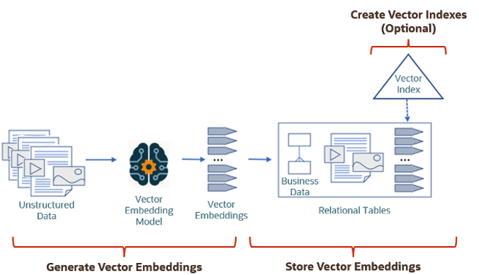
The first part involved creating Vectors for your existing data and for any new data generated and needs to be stored. This data can be used for Semantic Similarity searches (part two of the process). The first part of the process takes your data, applies a vector embedding model to it, generates the vectors and stores them in your Database. When the vectors are stored, Vector Indexes can be created.
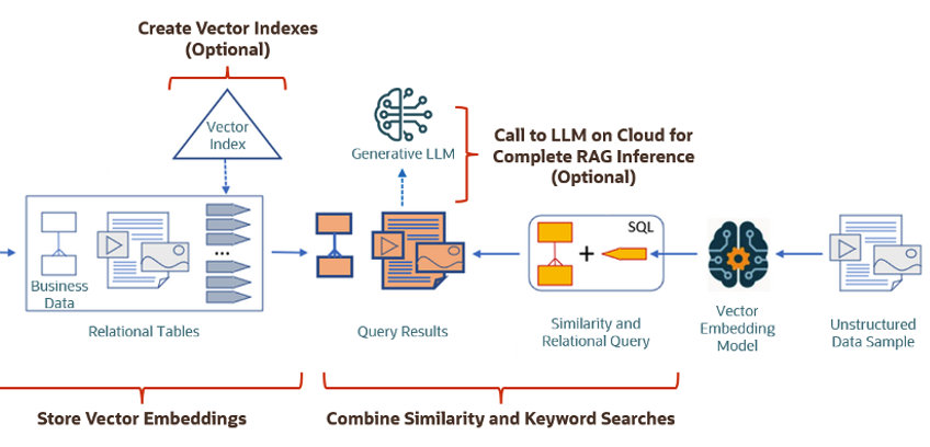
The second part if the process involves Vector Search. This involves having some data you want to search on (e.g. “CARS1” in the previous example). This data will need to be passed to the Vector Embedding model. A Vector for this data is generated. The Vector Search will use this vector to compare to all other vectors in the Database. The results returned will be those vectors (and their corresponding data) that closely match the vector being searched.
Check out my other posts in this series on Vector Databases.
Vector Databases – Part 1
A Vector Database is a specialized database designed to efficiently store, search, and retrieve high-dimensional vectors, which are often used to represent complex data like images, text, or audio. Vector Databases handle the growing need for managing unstructured and semi-structured data generated by AI models, particularly in applications such as recommendation systems, similarity search, and natural language processing. By enabling fast and scalable operations on vector embeddings, vector databases play a crucial role in unlocking the power of modern AI and machine learning applications.

While traditional Databases are very efficient with storing, processing and searching structured data, but over the past 10+ years they have expanded to include many of the typical NoSQL Database features. This allows ‘modern’ multi-model Databases to be capable of processing structured, semi-structured and unstructured data all within a single Database. Such NoSQL capabilities now available in ‘modern’ multi-model Databases include unstructured data, dynamic models, columnar data, in-memory data, distributed data, big data volumes, high performance, graph data processing, spatial data, documents, streaming, machine learning, artificial intelligence, etc. That is a long list of features and I haven’t listed everything. As new data processing paradigms emerge, they are evaluated and businesses identify the usefulness or not of each. If the new data processing paradigms are determined to be useful, apart from some niche use cases, these capabilities are integrated by the vendors of these ‘modern’ multi-model Database vendors. We have seen similar happen with Vector Databases over the past year or so. Yes Vector Databases have existed for many years but we now have the likes of Oracle, PostgreSQL, MySQL, SQL Server and even DB2 including Vector Embedding and Search.

Vector databases are specifically designed to store and search high-dimensional vector embeddings, which are generated by machine learning models. Here are some key use cases for vector databases:
1. Similarity Search:
- Image Search: Vector databases can be used to perform image similarity searches. For example, e-commerce platforms can allow users to search for products by uploading an image, and the system finds visually similar items using image embeddings.
- Document Search: In NLP (Natural Language Processing) tasks, vector databases help find semantically similar documents or text snippets by comparing their embeddings.
2. Recommendation Systems:
- Product Recommendations: Vector databases enable personalized product recommendations by comparing user and item embeddings to suggest items that are similar to a user’s past interactions or preferences.
- Content Recommendation: For media platforms (e.g., video streaming or news), vector databases power recommendation engines by finding content that matches the user’s interests based on embeddings of past behavior and content characteristics.
3. Natural Language Processing (NLP):
- Semantic Search: Vector databases are used in semantic search engines that understand the meaning behind a query, rather than just matching keywords. This is useful for applications like customer support or knowledge bases, where users may phrase questions in various ways.
- Question-Answering Systems: Vector databases can be employed to match user queries with relevant answers by comparing their vector representations, improving the accuracy and relevance of responses.
4. Anomaly Detection:
- Fraud Detection: In financial services, vector databases help detect anomalies or potential fraud by comparing transaction embeddings with a normal behavior profile.
- Security: Vector databases can be used to identify unusual patterns in network traffic or user behavior by comparing embeddings of normal activity to detect security threats.
5. Audio and Video Processing:
- Audio Search: Vector databases allow users to search for similar audio files or songs by comparing audio embeddings, which capture the characteristics of sound.
- Video Recommendation and Search: Embeddings of video content can be stored and queried in a vector database, enabling more accurate content discovery and recommendation in streaming platforms.
6. Geospatial Applications:
- Location-Based Services: Vector databases can store embeddings of geographical locations, enabling applications like nearest-neighbor search for finding the closest points of interest or users in a given area.
- Spatial Queries: Vector databases can be used in applications where spatial relationships matter, such as in logistics and supply chain management, where efficient searching of locations is crucial.
7. Biometric Identification:
- Face Recognition: Vector databases store face embeddings, allowing systems to compare and identify faces for authentication or security purposes.
- Fingerprint and Iris Matching: Similar to face recognition, vector databases can store and search biometric data like fingerprints or iris scans by comparing vector representations.
8. Drug Discovery and Genomics:
- Molecular Similarity Search: In the pharmaceutical industry, vector databases can help in searching for chemical compounds that are structurally similar to known drugs, aiding in drug discovery processes.
- Genomic Data Analysis: Vector databases can store and search genomic sequences, enabling fast comparison and clustering for research and personalized medicine.
9. Customer Support and Chatbots:
- Intelligent Response Systems: Vector databases can be used to store and retrieve relevant answers from a knowledge base by comparing user queries with stored embeddings, enabling more intelligent and context-aware responses in chatbots.
10. Social Media and Networking:
- User Matching: Social networking platforms can use vector databases to match users with similar interests, friends, or content, enhancing the user experience through better connections and content discovery.
- Content Moderation: Vector databases help in identifying and filtering out inappropriate content by comparing content embeddings with known examples of undesirable content.
These use cases highlight the versatility of vector databases in handling various applications that rely on similarity search, pattern recognition, and large-scale data processing in AI and machine learning environments.
This post is the first in a series on Vector Databases. Some will be background details and some will be technical examples using Oracle Database. I’ll post links to the following posts below as they are published.
OCI:Vision Template for Policies
When using OCI you’ll need to configure your account and other users to have the necessary privileges and permissions to run the various offerings. OCI Vision is no different. You have two options for doing this. The first is to manually configure these. There isn’t a lot to do but some issues can arise. The other option is to use a template. The OCI Vision team have created a template of what is required and I’ll walk through the steps of setting this up along with some additional steps you’ll need.
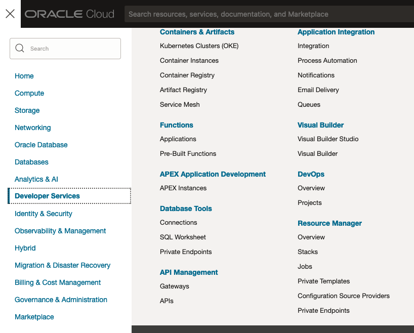
You’ll need to go to the Resource Manager page. This can be found under the menu by going to the Developer Services and then selecting Resource Manager.
First, you’ll need to go to the Resource Manager page. This can be found under the menu by going to the Developer Services and then selecting Resource Manager.
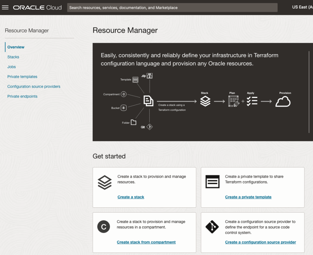
Located just under the main banner image you’ll see a section labelled ‘Create a stack’. Click on this link.
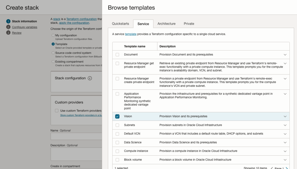
In the Create stack screen select Template from the radio group at the top of the page. Then in the Browse template pop-up screen, select the Service tab (across the top) and locate Vision. Once selected click the Select Template button.
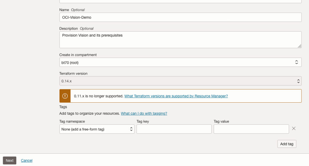
The page will load the necessary configuration. The only other thing you need to change on this page is the Name of the Service. Make it meaningful for you and your project. Click the Next button to continue to the next screen.
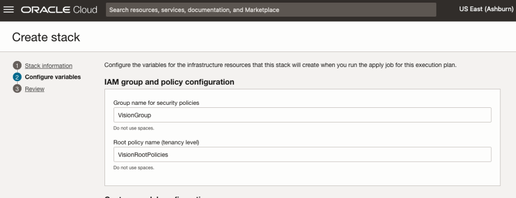
The top section relates to IAM Group name and policy configuration. You take the defaults or if you have specific groups already configured you can change it to it.
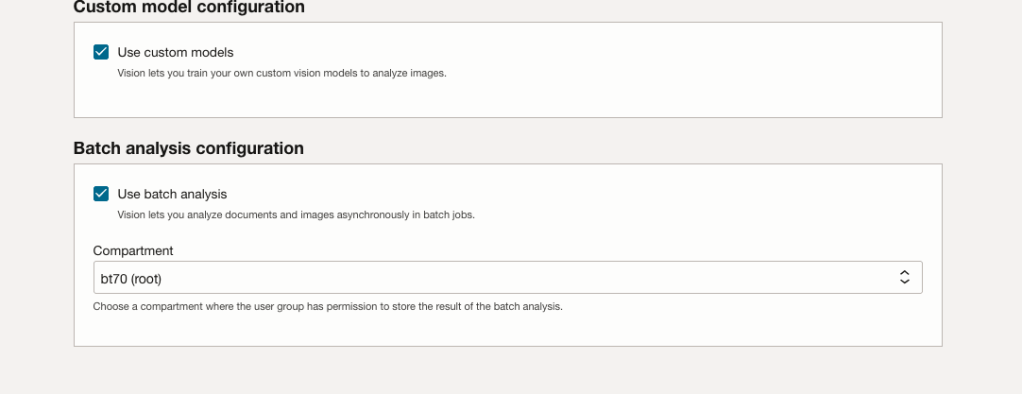
Most people will want to create their own customer models, as the supplied pre-built models are a bit basic. To enable Custom Built models, just tick the checkbox in the Custom Model Configuration section.
The second checkbox enables the batch processing of documents/images. If you check this box, you’ll need to specify the compartment you want the workload to be assigned to. Then click the Next button.
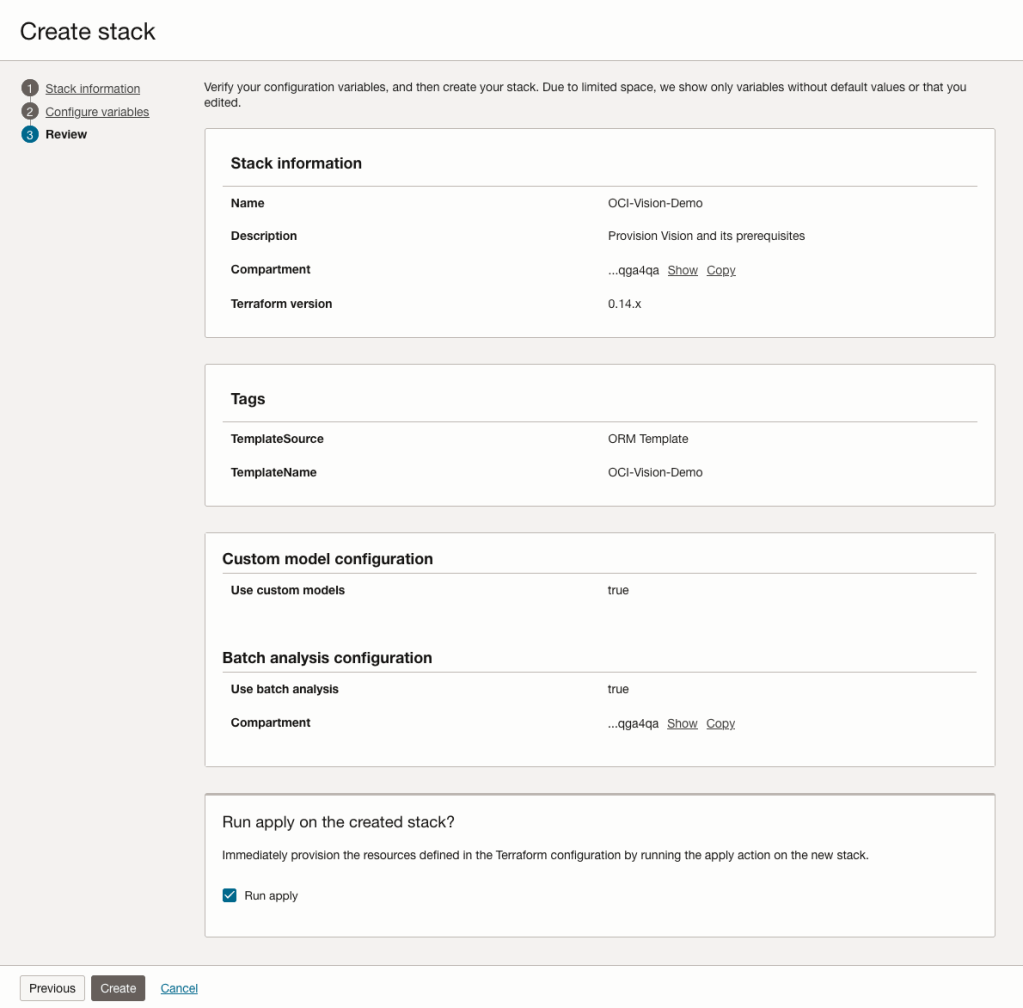
The final part displays a verification page of what was selected in the previous steps.
When ready click on the Run Apply check box and then click on the Create button.
It can take anything from a few seconds or a couple of minutes for the scripts to run.
When completed you’ll a Green box at the top of the screen and the message ‘SUCCEEDED’ under it.

Oracle 23c DBMS_SEARCH – Ubiquitous Search
One of the new PL/SQL packages with Oracle 23c is DBMS_SEARCH. This can be used for indexing (and searching) multiple schema objects in a single index.
Check out the documentation for DBMS_SEARCH.
This type of index is a little different to your traditional index. With DBMS_SEARCH we can create an index across multiple schema objects using just a single index. This gives us greater indexing capabilities for scenarios where we need to search data across multiple objects. You can create a ubiquitous search index on multiple columns of a table or multiple columns from different tables in a given schema. All done using one index, rather than having to use multiples. Because of this wider search capability, you will see this (DBMS_SEARCH) being referred to as a Ubiquitous Search Index. A ubiquitous search index is a JSON search index and can be used for full-text and range-based searches.
To create the index, you will first define the name of the index, and then add the different schema objects (tables, views) to it. The main commands for creating the index are:
- DBMS_SEARCH.CREATE_INDEX
- DBMS_SEARCH.ADD_SOURCE
Note: Each table used in the ADD_SOURCE must have a primary key.
The following is an example of using this type of index using the HR schema/data set.
exec dbms_search.create_index('HR_INDEX');This just creates the index header.
Important: For each index created using this method it will create a table with the Index name in your schemas. It will also create fourteen DR$ tables in your schema. SQL Developer filtering will help to hide these and minimise the clutter.
select table_name from user_tables;
...
HR_INDEX
DR$HR_INDEX$I
DR$HR_INDEX$K
DR$HR_INDEX$N
DR$HR_INDEX$U
DR$HR_INDEX$Q
DR$HR_INDEX$C
DR$HR_INDEX$B
DR$HR_INDEX$SN
DR$HR_INDEX$SV
DR$HR_INDEX$ST
DR$HR_INDEX$G
DR$HR_INDEX$DG
DR$HR_INDEX$KG
To add the contents and search space to the index we need to use ADD_SOURCE. In the following, I’m adding two tables to the index.
exec DBMS_SEARCH.ADD_SOURCE('HR_INDEX', 'EMPLOYEES');NOTE: At the time of writing this post some of the client tools and libraries do not support the JSON datatype fully. If they did, you could just query the index metadata, but until such time all tools and libraries fully support the data type, you will need to use the JSON_SERIALIZE function to translate the metadata. If you query the metadata and get no data returned, then try using this function to get the data.
Running a simple select from the index might give you an error due to the JSON type not being fully implemented in the client software. (This will change with time)
select * from HR_INDEX;But if we do a count from the index, we could get the number of objects it contains.
select count(*) from HR_INDEX;
   COUNT(*)
___________
        107
We can view what data is indexed by viewing the virtual document.
select json_serialize(DBMS_SEARCH.GET_DOCUMENT('HR_INDEX',METADATA))
from HR_INDEX;

JSON_SERIALIZE(DBMS_SEARCH.GET_DOCUMENT('HR_INDEX',METADATA))
___________________________________________________________________________________________________________________________________________________________________________________________________________________________________________________________________________
{"HR":{"EMPLOYEES":{"PHONE_NUMBER":"515.123.4567","JOB_ID":"AD_PRES","SALARY":24000,"COMMISSION_PCT":null,"FIRST_NAME":"Steven","EMPLOYEE_ID":100,"EMAIL":"SKING","LAST_NAME":"King","MANAGER_ID":null,"DEPARTMENT_ID":90,"HIRE_DATE":"2003-06-17T00:00:00"}}}
{"HR":{"EMPLOYEES":{"PHONE_NUMBER":"515.123.4568","JOB_ID":"AD_VP","SALARY":17000,"COMMISSION_PCT":null,"FIRST_NAME":"Neena","EMPLOYEE_ID":101,"EMAIL":"NKOCHHAR","LAST_NAME":"Kochhar","MANAGER_ID":100,"DEPARTMENT_ID":90,"HIRE_DATE":"2005-09-21T00:00:00"}}}
{"HR":{"EMPLOYEES":{"PHONE_NUMBER":"515.123.4569","JOB_ID":"AD_VP","SALARY":17000,"COMMISSION_PCT":null,"FIRST_NAME":"Lex","EMPLOYEE_ID":102,"EMAIL":"LDEHAAN","LAST_NAME":"De Haan","MANAGER_ID":100,"DEPARTMENT_ID":90,"HIRE_DATE":"2001-01-13T00:00:00"}}}
{"HR":{"EMPLOYEES":{"PHONE_NUMBER":"590.423.4567","JOB_ID":"IT_PROG","SALARY":9000,"COMMISSION_PCT":null,"FIRST_NAME":"Alexander","EMPLOYEE_ID":103,"EMAIL":"AHUNOLD","LAST_NAME":"Hunold","MANAGER_ID":102,"DEPARTMENT_ID":60,"HIRE_DATE":"2006-01-03T00:00:00"}}}
{"HR":{"EMPLOYEES":{"PHONE_NUMBER":"590.423.4568","JOB_ID":"IT_PROG","SALARY":6000,"COMMISSION_PCT":null,"FIRST_NAME":"Bruce","EMPLOYEE_ID":104,"EMAIL":"BERNST","LAST_NAME":"Ernst","MANAGER_ID":103,"DEPARTMENT_ID":60,"HIRE_DATE":"2007-05-21T00:00:00"}}}
We can search the metadata for certain data using the CONTAINS or JSON_TEXTCONTAINS functions.
select json_serialize(metadata)
from DEMO_IDX
where contains(data, 'winston')>0;
select json_serialize(metadata)
from DEMO_IDX
where json_textcontains(data, '$.HR.EMPLOYEES.FIRST_NAME', 'Winston');When the index is no longer required it can be dropped by running the following. Don’t run a DROP INDEX command as that removes some objects and leaves others behind! (leaves a bit of mess) and you won’t be able to recreate the index, unless you give it a different name.
exec dbms_search.drop_index('SH_INDEX');Oracle 23c Free – Developer Release
Oracle 23c if finally available, in the form of Oracle 23c FREE – Developer Release. There was lots of excitement in some parts of the IT community about this release, some of which is to do with people having to wait a while for this release, given 22c was never released due to Covid!
But some caution is needed and reining back on the excitement is needed.

Why? This release isn’t the full bells and whistles full release of 23c Database. There has been several people from Oracle emphasizing the name of this release is Oracle 23c Free – Developer Release. There are a few things to consider with this release. It isn’t a GA (General Available) Release which is due later this year (maybe). Oracle 23c Free – Developer Release is an early release to allow developers to start playing with various developer focused new features. Some people have referred to this as the 23c Beta version 2 release, and this can be seen in the DB header information. It could be viewed in a similar way as the XE releases we had previously. XE was always Free, so we now we have a rename and emphasis of this. These have been many, many organizations using the XE release to build applications. Also the the XE releases were a no cost option, or what most people would like to say, the FREE version.
For the full 23c Database release we will get even more features, but most of these will probably be larger enterprise scale scenarios.
Now it’s time you to go play with 23c Free – Developer Release. Here are some useful links
- Product Release Official Announcement
- Post by Gerald Venzi
- See link for Docker installation below
- VirtualBox Virtual Machine
- You want to do it old school – Download RPM files
- New Features Guide
I’ll be writing posts on some of the more interesting new features and I’ll add the links to those below. I’ll also add some links to post by other people:
- Docker Installation (Intel and Apple Chip)
- 23 Free Virtual Machine
- 23 Free – A Few (New Features) A few Quickies
- JSON Relational Duality – see post by Tim Hall
- more coming soon (see maintained list at https://oralytics.com/23c/)
Number of rows in each Table – Various Databases
A possible common task developers perform is to find out how many records exists in every table in a schema. In the examples below I’ll show examples for the current schema of the developer, but these can be expanded easily to include tables in other schemas or for all schemas across a database.
These example include the different ways of determining this information across the main databases including Oracle, MySQL, Postgres, SQL Server and Snowflake.
A little warning before using these queries. They may or may not give the true accurate number of records in the tables. These examples illustrate extracting the number of records from the data dictionaries of the databases. This is dependent on background processes being run to gather this information. These background processes run from time to time, anything from a few minutes to many tens of minutes. So, these results are good indication of the number of records in each table.
Oracle
SELECT table_name, num_rows
FROM user_tables
ORDER BY num_rows DESC;
or
SELECT table_name,
       to_number(
          extractvalue(xmltype(
             dbms_xmlgen.getxml('select count(*) c from '||table_name))
                ,'/ROWSET/ROW/C')) tab_count
FROM   user_tables
ORDER BY tab_count desc;
Using PL/SQL we can do something like the following.
DECLARE
   val NUMBER;
BEGIN
   FOR i IN (SELECT table_name FROM user_tables ORDER BY table_name desc) LOOP
      EXECUTE IMMEDIATE 'SELECT count(*) FROM '|| i.table_name INTO val;
      DBMS_OUTPUT.PUT_LINE(i.table_name||' -> '|| val );
   END LOOP;
END;
MySQL
SELECT table_name, table_rows
FROM INFORMATION_SCHEMA.TABLES
WHERE table_type = 'BASE TABLE'
AND  TABLE_SCHEMA = current_user();
Using Common Table Expressions (CTE), using WITH clause
WITH table_list AS (
SELECT
    table_name
  FROM information_schema.tables
  WHERE table_schema = current_user()
  AND
        table_type = 'BASE TABLE'
)
SELECT CONCAT(
            GROUP_CONCAT(CONCAT("SELECT '",table_name,"' table_name,COUNT(*) rows FROM ",table_name) SEPARATOR " UNION "),
            ' ORDER BY table_name'
        )
INTO @sql
FROM table_list;
Postgres
select relname as table_name, n_live_tup as num_rows from pg_stat_user_tables;
An alternative is
select n.nspname as table_schema,
       c.relname as table_name,
       c.reltuples as rows
from pg_class c
join pg_namespace n on n.oid = c.relnamespace
where c.relkind = 'r'
      and n.nspname = current_user
order by c.reltuples desc;
SQL Server
SELECT tab.name,
       sum(par.rows)
FROM   sys.tables tab INNER JOIN sys.partitions par
          ON tab.object_id = par.object_id
WHERE  schema_name(tab.schema_id) = current_user
Snowflake
SELECT t.table_schema, t.table_name, t.row_count
FROM   information_schema.tables t
WHERE  t.table_type = 'BASE TABLE'
AND    t.table_schema = current_user
order by t.row_count desc;
The examples give above are some of the ways to obtain this information. As with most things, there can be multiple ways of doing it, and most people will have their preferred one which is based on their background and preferences.
As you can see from the code given above they are all very similar, with similar syntax, etc. The only thing different is the name of the data dictionary table/view containing the information needed. Yes, knowing what data dictionary views to query can be a little challenging as you switch between databases.
AUTO_PARTITION – Inspecting & Implementing Recommendations
In a previous blog post I gave an overview of the DBMS_AUTO_PARTITION package in Oracle Autonomous Database. This looked at how you can get started and to setup Auto Partitioning and to allow it to automatically implement partitioning.
This might not be something the DBAs will want to happen for lots of different reasons. An alternative is to use DBMS_AUTO_PARTITION to make recommendations for tables where partitioning will have a performance improvement. The DBA can inspect these recommendations and decide which of these to implement.
In the previous post we set the CONFIGURE function to be ‘IMPLEMENT’. We need to change that to report the recommendations.
exec dbms_auto_partition.configure('AUTO_PARTITION_MODE','REPORT ONLY');Just remember, tables will only be considered by AUTO_PARTITION as outlined in my previous post.
Next we can ask for recommendations using the RECOMMEND_PARTITION_METHOD function.
exec  dbms_auto_partition.recommend_partition_method(
   table_owner => 'WHISKEY',
   table_name => 'DIRECTIONS',
   report_type => 'TEXT',
   report_section => 'ALL',
   report_level => 'ALL');
The results from this are stored in DBA_AUTO_PARTITION_RECOMMENDATIONS, which you can query to view the recommendations.
select recommendation_id, partition_method, partition_key
from dba_auto_partition_recommendations;
RECOMMENDATION_ID PARTITION_METHOD PARTITION_KEY
-------------------------------- ------------------------------------------------------------------------------------------------------------- --------------
D28FC3CF09DF1E1DE053D010000ABEA6 Method: LIST(SYS_OP_INTERVAL_HIGH_BOUND("D", INTERVAL '2' MONTH, TIMESTAMP '2019-08-10 00:00:00')) AUTOMATIC D
To apply the recommendation pass the RECOMMENDATION_KEY value to the APPLY_RECOMMENDATION function.
exec dbms_auto_partition.apply_recommendation('D28FC3CF09DF1E1DE053D010000ABEA6');It might takes some minutes for the partitioned table to become available. During this time the original table will remain available as the change will be implemented using a ALTER TABLE MODIFY PARTITION ONLINE command.
Two other functions include REPORT_ACTIVITY and REPORT_LAST_ACTIVITY. These can be used to export a detailed report on the recommendations in text or HTML form. It is probably a good idea to create and download these for your change records.
spool autoPartitionFinding.html
select dbms_auto_partition.report_last_activity(type=>'HTML') from dual;
exit;
You must be logged in to post a comment.