
Vector Embeddings
How to access and use Multilingual embedding models using OML for Python 2.1
With the release of OML for Python 2.1, we have a newer approach for accessing and generating embedding models in ONNX format (from Hugging Face), which can then be loaded into the Database (>=23.7ai). Although with this newer approach, we need to be aware of the previous way of doing it (<=23.6). As of 23.7ai this previous approach is now deprecated. Given the short time the previous approach was around, things could yet change with subsequent releases.
As the popularity of Vector Search spreads, there have been some challenges relating to obtaining and using suitable models within a Database. Oracle 23ai introduced the ability to load an embedding model in ONNX format into the database. These could be easily used to create and update embedding vectors for your data. But there were some limitations and challenges with what ONNX models could be used, and sometimes this was limited to the formatting of the ONNX metadata and the pretrained models themselves.
To ease the process of locating, converting and loading an embedding model into an Oracle Database, Oracle Machine Learning for Python 2.1 has been released with some new features and methods to make the process slightly easier. There are three constraints for doing this: 1) you need to use Oracle Machine Learning for Python 2.1 (OML4Py 2.1), and 2) you need to use Oracle 23.7ai (or greater) Database (This later requirement is to allow for the expanded range of embedding models) and 3) Python 3.12 (or greater).
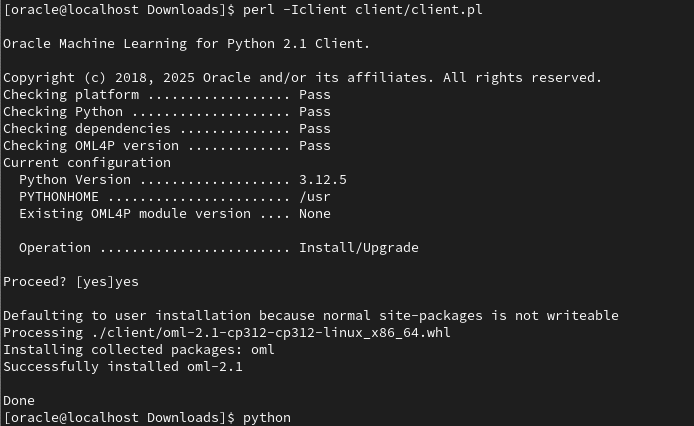
There are a few additional Python libraries needed, so check the documentation for more details on what the most recent version of these should be. But do be careful of the documentation as the version I followed there was some inconsistencies in different sections regarding the requirements and steps to follow for installation. Hopefully this will be tidied up by the time you read the documentation.
With OML4Py 2.1 there is a class called oml.utils.onnxpipeline, with a number of methods to support the exploration of preconfigured models. These include: from_preconfigured(), from_template() and show_preconfigured(). This last one displays the list of preconfigured models.
oml.ONNXPipelineConfig.show_preconfigured()
['sentence-transformers/all-mpnet-base-v2', 'sentence-transformers/all-MiniLM-L6-v2', 'sentence-transformers/multi-qa-MiniLM-L6-cos-v1', 'sentence-transformers/distiluse-base-multilingual-cased-v2', 'sentence-transformers/all-MiniLM-L12-v2', 'BAAI/bge-small-en-v1.5', 'BAAI/bge-base-en-v1.5', 'taylorAI/bge-micro-v2', 'intfloat/e5-small-v2', 'intfloat/e5-base-v2', 'thenlper/gte-base', 'thenlper/gte-small', 'TaylorAI/gte-tiny', 'sentence-transformers/paraphrase-multilingual-mpnet-base-v2', 'intfloat/multilingual-e5-base', 'intfloat/multilingual-e5-small', 'sentence-transformers/stsb-xlm-r-multilingual', 'Snowflake/snowflake-arctic-embed-xs', 'Snowflake/snowflake-arctic-embed-s', 'Snowflake/snowflake-arctic-embed-m', 'mixedbread-ai/mxbai-embed-large-v1', 'openai/clip-vit-large-patch14', 'google/vit-base-patch16-224', 'microsoft/resnet-18', 'microsoft/resnet-50', 'WinKawaks/vit-tiny-patch16-224', 'Falconsai/nsfw_image_detection', 'WinKawaks/vit-small-patch16-224', 'nateraw/vit-age-classifier', 'rizvandwiki/gender-classification', 'AdamCodd/vit-base-nsfw-detector', 'trpakov/vit-face-expression', 'BAAI/bge-reranker-base']
We can inspect the full details of all models or for an individual model by changing some of the parameters.
oml.ONNXPipelineConfig.show_preconfigured(include_properties=True, model_name='microsoft/resnet-50')
[{'checksum': 'fca7567354d0cb0b7258a44810150f7c1abf8e955cff9320b043c0554ba81f8e', 'model_type': 'IMAGE_CONVNEXT', 'pre_processors_img': [{'name': 'DecodeImage', 'do_convert_rgb': True}, {'name': 'Resize', 'enable': True, 'size': {'height': 384, 'width': 384}, 'resample': 'bilinear'}, {'name': 'Rescale', 'enable': True, 'rescale_factor': 0.00392156862}, {'name': 'Normalize', 'enable': True, 'image_mean': 'IMAGENET_STANDARD_MEAN', 'image_std': 'IMAGENET_STANDARD_STD'}, {'name': 'OrderChannels', 'order': 'CHW'}], 'post_processors_img': []}]
Let’s prepare a preconfigured model using the simplest approach. In this example we’ll use the 'sentence-transformers/multi-qa-MiniLM-L6-cos-v1' model. Start by defining a pipeline.
pipeline = oml.utils.ONNXPipeline(model_name="sentence-transformers/multi-qa-MiniLM-L6-cos-v1")We now have the choice of loading it straight to your database using an already established OML connection.
pipeline.export2db("my_onnx_model_db")or you can export the model to a file
pipeline.export2file("my_onnx_model", output_dir="/home/oracle/onnx")
When you check the file system, you’ll see something like the following. Depending on the model you exported and any configuration changes to the model, the file size will vary in size.
-rw-r--r--. 1 oracle oracle 90636512 Apr 22 12:00 my_onnx_model.onnxIs you ran the export2file() function you’ll need to move that file to the database server. This will involve talking gently with the DBA to get their assistance. Once permission is obtained from the DBA, the ONNX file will be copied into a directory that is referenced from within the database. This is a simple task of defining an external file system directory where the file is located. In the example below the directory is referenced as ONNX_DIR. This is the reference defined in the database, which has a pointer to directory on the file system. The next task is to load the ONNX file into your Database schema.
BEGIN
   DBMS_VECTOR.LOAD_ONNX_MODEL(
        directory => 'ONNX_DIR',
        file_name => 'my_onnx_model.onnx',
        model_name => 'Multi-qa-MiniLM-L6-Cos-v1');
END;
Once loaded the model can be used to create Vector Embeddings.
Vector Databases – Part 4 – Vector Indexes
In this post on Vector Databases, I’ll explore some of the commonly used indexing techniques available in Databases. I’ll also explore the Vector Indexes available in Oracle 23c. Be sure to check that section towards the end of the post, where I’ll also include links to other articles in this series.
As with most data in a Databases, indexes are used for fast access to data. They create an organised structure (typically B+ tree) for storing the location of certain values within a table. When searching for data, if an index exists on that data, the index will be used for matching and the location of the records is used to quickly retrieve the data.
Similarly, for Vector searches, we need some way to search through thousands or millions of vectors to find those that best match our search criteria (vector search). For vector search, there are many more calculations to perform. We want to avoid a MxN search space.

Given the nature of Vectors and the the type of search performed on these, databases need to have different types of indexes. Common Vector Index types include Hash-base, Tree-based, Graph-base and Inverted-file. Let’s have a look at each of these.

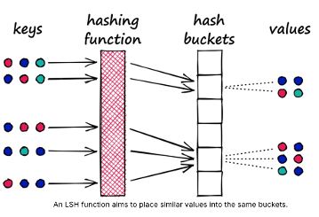
Hash-based Vector Indexes
Locality-Sensitive Hashing (LSH) uses hash functions to bucket similar vectors into a hash table. The query vectors are also hashed using the same hash function and it is compared with the other vectors already present in the table. This method is much faster than doing an exhaustive search across the entire dataset because there are fewer vectors in each hash table than in the whole vector space. While this technique is quite fast, the downside is that it is not very accurate. LSH is an approximate method, so a better hash function will result in a better approximation, but the result will not be the exact answer.
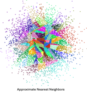
Tree-based Vector Indexes
Tree-based indexing allows for fast searches by using a data structure such as a binary tree. The tree gets created in a way that similar vectors are grouped in the same subtree. Approximate Nearest Neighbour (ANN) uses a forest of binary trees to perform approximate nearest neighbors search. ANN performs well with high-dimension data where doing an exact nearest neighbors search can be expensive. The downside of using this method is that it can take a significant amount of time to build the index. Whenever a new data point is received, the indices cannot be restructured on the fly. The entire index has to be rebuilt from scratch.
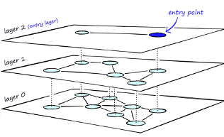
Graph-based Vector Indexes
Similar to tree-based indexing, graph-based indexing groups similar data points by connecting them with an edge. Graph-based indexing is useful when trying to search for vectors in a high-dimensional space. Hierarchical Navigable Small Worlds (HNSW) creates a layered graph with the topmost layer containing the fewest points and the bottom layer containing the most points. When an input query comes in, the topmost layer is searched via ANN. The graph is traversed downward layer by layer. At each layer, the ANN algorithm is run to find the closest point to the input query. Once the bottom layer is hit, the nearest point to the input query is returned. Graph-based indexing is very efficient because it allows one to search through a high-dimensional space by narrowing down the location at each layer. However, re-indexing can be challenging because the entire graph may need to be recreated
Inverted-FIle Vector Indexes
IVF (InVerted File) narrows the search space by partitioning the dataset and creating a centroid(random point) for each partition. The centroids get updated via the K-Means algorithm. Once the index is populated, the ANN algorithm finds the nearest centroid to the input query and only searches through that partition. Although IVF is efficient at searching for similar points once the index is created, the process of creating the partitions and centroids can be quite slow.

Oracle 23ai comes with two main types of indexes for Vectors. These are:
In-Memory – Neighbor Graph Vector Index
Hierarchical Navigable Small World (HNSW) is the only type of In-Memory Neighbor Graph vector index supported. With Navigable Small World (NSW), the idea is to build a proximity graph where each vector in the graph connects to several others based on three characteristics:
- The distance between vectors
- The maximum number of closest vector candidates considered at each step of the search during insertion (EFCONSTRUCTION)
- Within the maximum number of connections (NEIGHBORS) permitted per vector
Navigable Small World (NSW) graph traversal for vector search begins with a predefined entry point in the graph, accessing a cluster of closely related vectors. The search algorithm employs two key lists:
- Candidates, a dynamically updated list of vectors that we encounter while traversing the graph,
- and Results, which contains the vectors closest to the query vector found thus far.
As the search progresses, the algorithm navigates through the graph, continually refining the Candidates by exploring and evaluating vectors that might be closer than those in the Results. The process concludes once there are no vectors in the Candidates closer than the farthest in the Results, indicating

Neighbor Partition Vector Index
Inverted File Flat (IVF) index is the only type of Neighbor Partition vector index supported.
Inverted File Flat Index (IVF Flat or simply IVF) is a partitioned-based index which balance high search quality with reasonable speed.
The IVF index is a technique designed to enhance search efficiency by narrowing the search area through the use of neighbor partitions or clusters.

Here is an example of creating such an index in Oracle 23ai.
CREATE VECTOR INDEX galaxies_ivf_idx ON galaxies (embedding)
ORGANIZATION NEIGHBOR
PARTITIONS DISTANCE COSINE
WITH TARGET ACCURACY 95;
Check out my other posts in this series on Vector Databases.
Vector Databases – Part 3 – Vector Search
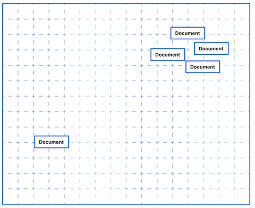
Searching semantic similarity in a data set is now equivalent to searching for nearest neighbors in a vector space instead of using traditional keyword searches using query predicates. The distance between “dog” and “wolf” in this vector space is shorter than the distance between “dog” and “kitten”. A “dog” is more similar to a “wolf” than it is to a “kitten”.

Vector data tends to be unevenly distributed and clustered into groups that are semantically related. Doing a similarity search based on a given query vector is equivalent to retrieving the K-nearest vectors to your query vector in your vector space.
Typically, you want to find an ordered list of vectors by ranking them, where the first row in the list is the closest or most similar vector to the query vector, the second row in the list is the second closest vector to the query vector, and so on. When doing a similarity search, the relative order of distances is what really matters rather than the actual distance.

Semantic search where the initial vector is the word “Puppy” and you want to identify the four closest words. Similarity searches tend to get data from one or more clusters depending on the value of the query vector, distance and the fetch size. Approximate searches using vector indexes can limit the searches to specific clusters, whereas exact searches visit vectors across all clusters.
Measuring distances in a vector space is the core of identifying the most relevant results for a given query vector. That process is very different from the well-known keyword filtering in the relational database world, which is very quick, simple and very very efficient. Vector distance functions involve more complicated computations.
There are several ways you can calculate distances to determine how similar, or dissimilar, two vectors are. Each distance metric is computed using different mathematical formulas. The time taken to calculate the distance between two vectors depends on many factors, including the distance metric used as well as the format of the vectors themselves, such as the number of vector dimensions and the vector dimension formats.
Generally, it’s best to match the distance metric you use to the one that was used to train the vector embedding model that generated the vectors. Common Distance metric functions include:
- Euclidean Distance
- Euclidean Distance Squared
- Cosine Similarity [most commonly used]
- Dot Product Similarity
- Manhattan Distance Hamming Similarity
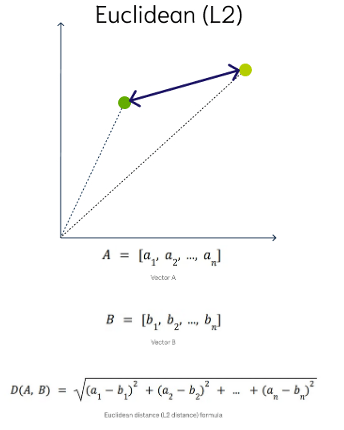
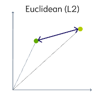
Euclidean Distance
This is a measure of the straight line distance between two points in the vector space. It ranges from 0 to infinity, where 0 represents identical vectors, and larger values represent increasingly dissimilar vectors. This is calculated using the Pythagorean theorem applied to the vector’s coordinates.
This metric is sensitive to both the vector’s size and it’s direction.
Euclidean Distance Squared
This is very similar to Euclidean Distance. When ordering is more important than the distance values themselves, the Squared Euclidean distance is very useful as it is faster to calculate than the Euclidean distance (avoiding the square-root calculation)
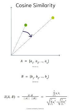
Cosine Similarity
This is the most commonly used distance measure. The cosine of the angle between two vectors – the larger the cosine, the closer the vectors. The smaller the angle, the bigger is its cosine. Cosine similarity measures the similarity in the direction or angle of the vectors, ignoring differences in their size (also called magnitude). The smaller the angle, the more similar are the two vectors. It ranges from -1 to 1, where 1 represents identical vectors, 0 represents orthogonal vectors, and -1 represents vectors that are diametrically opposed
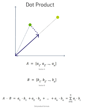
DOT Product Similarity
DOT product similarity of two vectors can be viewed as multiplying the size of each vector by the cosine of their angle. The larger the dot product, the closer the vectors. You project one vector on the other and multiply the resulting vector sizes. Larger DOT product values imply that the vectors are more similar, while smaller values imply that they are less similar. It ranges from -∞ to ∞, where a positive value represents vectors that point in the same direction, 0 represents orthogonal vectors, and a negative value represents vectors that point in opposite directions
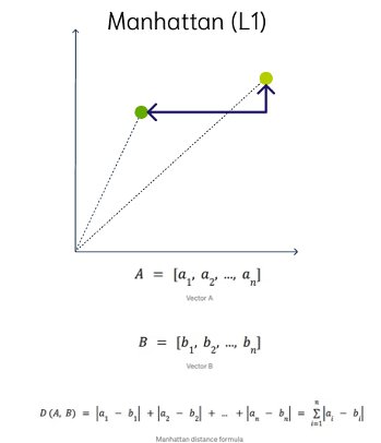
Manhattan Distance
This is calculated by summing the distance between the dimensions of the two vectors that you want to compare.
Imagine yourself in the streets of Manhattan trying to go from point A to point B. A straight line is not possible.
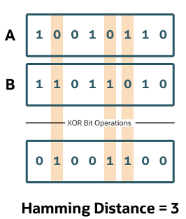
Hamming Similarity
This is the distance between two vectors represented by the number of dimensions where they differ. When using binary vectors, the Hamming distance between two vectors is the number of bits you must change to change one vector into the other. To compute the Hamming distance between two vectors, you need to compare the position of each bit in the sequence.
Check out my other posts in this series on Vector Databases.
Vector Databases – Part 2
In this post on Vector Databases, I’ll look at the main components:
- Vector Embedding Models. What they do and what they create.
- Vectors. What they represent, and why they have different sizes.
- Vector Search. An overview of what a Vector Search will do. A more detailed version of this is in a separate post.
- Vector Search Process. It’s a multi-step process and some care is needed.

Vector Embedding Models
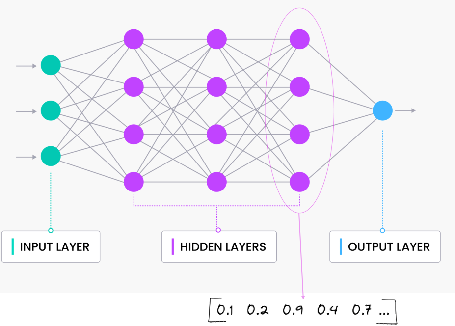
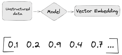
A vector embedding model is a type of machine learning model that transforms data into vectors (embeddings) in a high-dimensional space. These embeddings capture the semantic or contextual relationships between the data points, making them useful for tasks such as similarity search, clustering, and classification.
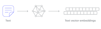
Embedding models are trained to convert the input data point (text, video, image, etc) into a vector (a series of numeric values). The model aims to identify semantic similarity with the input and map these to N-dimensional space. For example, the words “car” and “vehicle” have very different spelling but are semantically similar. The embedding model should map this to have similar vectors. Similarly with documents. The embedding model will map the documents to be able to group similar documents together (in N-dimensional space).
An embedding model is typically a Neural Network (NN) model. There are many different embedding models available from various vendor such as OpenAI, Cohere, etc., or you can build your own. Some models are open source and some are available for a fee. Typically, the output from the embedding model (the Vector) come from the last layer of the neural network
Vectors
A Vector is a sequence of numbers, called dimensions, used to capture the important “features” or “characteristics” of a piece of data. A vector is a mathematical object that has both magnitude (length) and direction. In the context of mathematics and physics, a vector is typically represented as an arrow pointing from one point to another in space, or as a list of numbers (coordinates) that define its position in a particular space.
Different Embedding Models create different numbers of Dimensions. Size is important with vectors as the greater the number number of dimensions the larger the Vector. The larger the number of dimensions the better the semantic similarity matches will be. As Vector size increases, so does space required to store them (not really a problem for Databases, but at Big Data scale it can be a challenge)
As vector size increases so does the Index space, and correspondingly search time can increase as the number of calculations for Distance Measure increases. There are various Vector indexes available to help with this (see my post covering this topic)
Basically, a vector is an array of numbers, where each number represents a dimension. It is easy for us to comprehend and visualise 2 dimensions. Here is an example of using 2 dimensions to represent different types of vehicles. The vectors give us a way to map or chart the data.
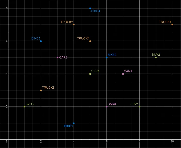
Here is SQL code for this data. I’ll come back to this data in the section on Vector Search.
INSERT INTO PARKING_LOT VALUES('CAR1','[7,4]');
INSERT INTO PARKING_LOT VALUES('CAR2','[3,5]');
INSERT INTO PARKING_LOT VALUES('CAR3','[6,2]');
INSERT INTO PARKING_LOT VALUES('TRUCK1','[10,7]');
INSERT INTO PARKING_LOT VALUES('TRUCK2','[4,7]');
INSERT INTO PARKING_LOT VALUES('TRUCK3','[2,3]');
INSERT INTO PARKING_LOT VALUES('TRUCK4','[5,6]');
INSERT INTO PARKING_LOT VALUES('BIKE1','[4,1]');
INSERT INTO PARKING_LOT VALUES('BIKE2','[6,5]');
INSERT INTO PARKING_LOT VALUES('BIKE3','[2,6]');
INSERT INTO PARKING_LOT VALUES('BIKE4','[5,8]');
INSERT INTO PARKING_LOT VALUES('SUV1','[8,2]');
INSERT INTO PARKING_LOT VALUES('SUV2','[9,5]');
INSERT INTO PARKING_LOT VALUES('SUV3','[1,2]');
INSERT INTO PARKING_LOT VALUES('SUV4','[5,4]');
The vectors created by the embedding models can have a different number of dimensions. Common Dimension Sizes are:
- 100-Dimensional: Often used in older or simpler models like some configurations of Word2Vec and GloVe. Suitable for tasks where computational efficiency is a priority and the context isn’t highly complex.
- 300-Dimensional: A common choice for many word embeddings (e.g., Word2Vec, GloVe). Strikes a balance between capturing sufficient detail and computational feasibility.
- 512-Dimensional: Used in some transformer models and sentence embeddings. Offers a richer representation than 300-dimensional embeddings.
- 768-Dimensional: Standard for BERT base models and many other transformer-based models. Provides detailed and contextual embeddings suitable for complex tasks.
- 1024-Dimensional: Used in larger transformer models (e.g., GPT-2 large). Provides even more detail but requires more computational resources.
Many of the newer embedding models have >3000 dimensions!
- Cohere’s embedding model embed-english-v3.0 has 1024 dimensions.
- OpenAI’s embedding model text-embedding-3-large has 3072 dimensions.
- Hugging Face’s embedding model all-MiniLM-L6-v2 has 384 dimensions
Here is a blog post listing some of the embedding models supported by Oracle Vector Search.
Vector Search
Vector search is a method of retrieving data by comparing high-dimensional vector representations (embeddings) of items rather than using traditional keyword or exact-match queries. This technique is commonly used in applications that involve similarity search, where the goal is to find items that are most similar to a given query based on their vector representations.
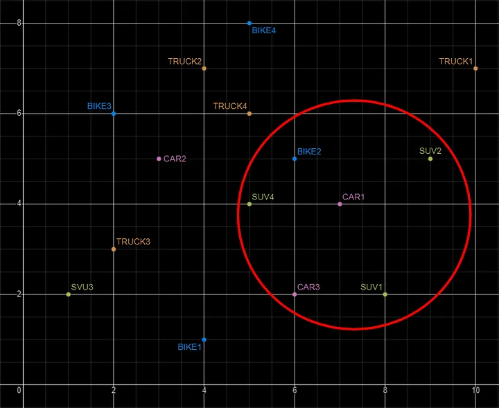
For example, using the vehicle data given above, we can easily visualise the search for similar vehicles. If we took “CAR1” as our initiating data point and wanted to know what other vehicles are similar to it. Vector Search looks at the distance between “CAR1” and all other vehicles in the 2-dimensional space.
Vector Search becomes a bit more of a challenge when we have 1000+ dimensions, requiring advanced distance algorithms. I’ll have more on these in the next post.
Vector Search Process
The Vector Search process is divided into two parts.
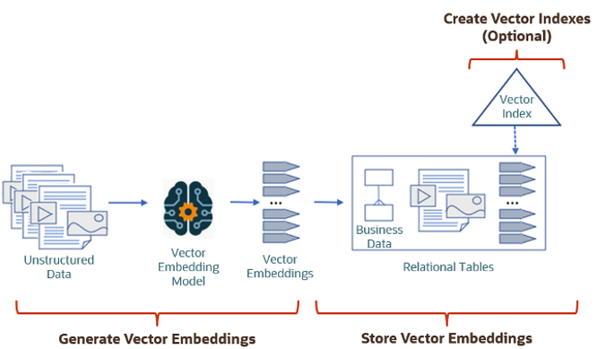
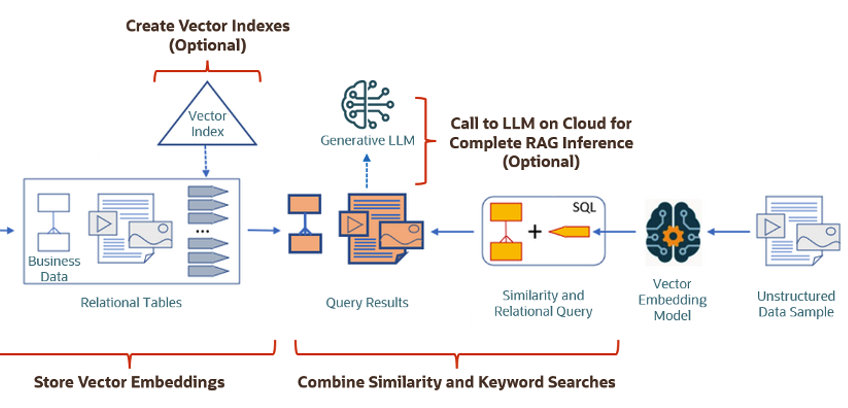
The first part involved creating Vectors for your existing data and for any new data generated and needs to be stored. This data can be used for Semantic Similarity searches (part two of the process). The first part of the process takes your data, applies a vector embedding model to it, generates the vectors and stores them in your Database. When the vectors are stored, Vector Indexes can be created.
The second part if the process involves Vector Search. This involves having some data you want to search on (e.g. “CARS1” in the previous example). This data will need to be passed to the Vector Embedding model. A Vector for this data is generated. The Vector Search will use this vector to compare to all other vectors in the Database. The results returned will be those vectors (and their corresponding data) that closely match the vector being searched.
Check out my other posts in this series on Vector Databases.
Using OpenAI to Generate Vector Embeddings
In a recent post, I demonstrated how you could use Cohere to generate Vector Embeddings. Despite having upgraded to a Production API (i.e. a paid one), the experience and time taken to process a relatively small dataset was underwhelming. The result was Cohere wasn’t up to the job of generating Vector Embeddings for the dataset, never mind a few hundred records of that dataset.
This post explores using OpenAI to perform the same task.
First thing is to install the OpenAI python library
pip install openaiNext, you need to create an account with OpenAI. This will allow you to get an API key. OpenAI gives you greater access to and usage of their algorithms than Cohere. Their response times are quicker and you have to lots before any rate limiting might kick in.
Using the same Wine Reviews dataset, the following code processes the data in the same/similar using the OpenAI embedding models. OpenAI has three text embedding models and these create vector embeddings with up to 1536 dimensions, or if you use the large model it will have 3072 dimensions. However, with these OpenAI Embedding models, you can specify a small number of dimensions, which gives you flexibility based on your datasets and the problems being addressed. It also allows you to be more careful with the space allocation for the vector embeddings and the vector indexes created on these.
One other setup you need to do to use the OpenAI API is to create a local environment variable. You can do this at the terminal level, or set/define it in your Python code, as shown below.
import openai
import os
import numpy as np
import os
import time
import pandas as pd

print_every = 200
num_records = 10000

#define your OpenAI API Key
os.environ["OPENAI_API_KEY"] = "... Your OpenAI API Key ..."

client = openai.OpenAI()

#load file into pandas DF
data_file = '.../winemag-data-130k-v2.csv'
df = pd.read_csv(data_file)

#define the outfile name
print("Input file :", data_file)
v_file = os.path.splitext(data_file)[0]+'.openai'
print(v_file)

#Open file with write (over-writes previous file)
f=open(v_file,"w")
f.write("delete from WINE_REVIEWS_130K;\n")
for index,row in df.head(num_records).iterrows():
    response = client.embeddings.create(
        model = "text-embedding-3-large",
        input = row['description'],
        dimensions = 100
    )
    v_embedding = str(response.data[0].embedding)
    tab_insert="INSERT into WINE_REVIEWS_130K VALUES ("+str(row["Seq"])+"," \
        +"'"+str(row["country"])+"'," \
        +"'"+str(row["description"])+"'," \
        +"'"+str(row["designation"])+"'," \
        +str(row["points"])+"," \
        +str(row["price"])+"," \
        +"'"+str(row["province"])+"'," \
        +"'"+str(row["region_1"])+"'," \
        +"'"+str(row["region_2"])+"'," \
        +"'"+str(row["taster_name"])+"'," \
        +"'"+str(row["taster_twitter_handle"])+"'," \
        +"'"+str(row["title"])+"'," \
        +"'"+str(row["variety"])+"'," \
        +"'"+str(row["winery"])+"'," \
        +"'"+v_embedding+"'"+");\n"

#    print(tab_insert)

    f.write(tab_insert)
    if (index%print_every == 0):
        print(f'Processed {index} vectors ', time.strftime("%H:%M:%S", time.localtime()))


#Close vector file
f.write("commit;\n")
f.close()
print(f"Finished writing file with Vector data [{index+1} vectors]", time.strftime("%H:%M:%S", time.localtime()))
That’s it. You can now run the script file to populate the table in your Database.
I mentioned above in in my previous post about using Cohere for this task. Yes there were some issues when using Cohere but for OpenAI everything ran very smoothly and was much. quicker too. I did encounter some rate limiting with OpenAI when I tried to processs more than ten thousand records. But the code did eventually complete.
Here is an example of the output from one of my tests.

Vector Databases – Part 1
A Vector Database is a specialized database designed to efficiently store, search, and retrieve high-dimensional vectors, which are often used to represent complex data like images, text, or audio. Vector Databases handle the growing need for managing unstructured and semi-structured data generated by AI models, particularly in applications such as recommendation systems, similarity search, and natural language processing. By enabling fast and scalable operations on vector embeddings, vector databases play a crucial role in unlocking the power of modern AI and machine learning applications.

While traditional Databases are very efficient with storing, processing and searching structured data, but over the past 10+ years they have expanded to include many of the typical NoSQL Database features. This allows ‘modern’ multi-model Databases to be capable of processing structured, semi-structured and unstructured data all within a single Database. Such NoSQL capabilities now available in ‘modern’ multi-model Databases include unstructured data, dynamic models, columnar data, in-memory data, distributed data, big data volumes, high performance, graph data processing, spatial data, documents, streaming, machine learning, artificial intelligence, etc. That is a long list of features and I haven’t listed everything. As new data processing paradigms emerge, they are evaluated and businesses identify the usefulness or not of each. If the new data processing paradigms are determined to be useful, apart from some niche use cases, these capabilities are integrated by the vendors of these ‘modern’ multi-model Database vendors. We have seen similar happen with Vector Databases over the past year or so. Yes Vector Databases have existed for many years but we now have the likes of Oracle, PostgreSQL, MySQL, SQL Server and even DB2 including Vector Embedding and Search.

Vector databases are specifically designed to store and search high-dimensional vector embeddings, which are generated by machine learning models. Here are some key use cases for vector databases:
1. Similarity Search:
- Image Search: Vector databases can be used to perform image similarity searches. For example, e-commerce platforms can allow users to search for products by uploading an image, and the system finds visually similar items using image embeddings.
- Document Search: In NLP (Natural Language Processing) tasks, vector databases help find semantically similar documents or text snippets by comparing their embeddings.
2. Recommendation Systems:
- Product Recommendations: Vector databases enable personalized product recommendations by comparing user and item embeddings to suggest items that are similar to a user’s past interactions or preferences.
- Content Recommendation: For media platforms (e.g., video streaming or news), vector databases power recommendation engines by finding content that matches the user’s interests based on embeddings of past behavior and content characteristics.
3. Natural Language Processing (NLP):
- Semantic Search: Vector databases are used in semantic search engines that understand the meaning behind a query, rather than just matching keywords. This is useful for applications like customer support or knowledge bases, where users may phrase questions in various ways.
- Question-Answering Systems: Vector databases can be employed to match user queries with relevant answers by comparing their vector representations, improving the accuracy and relevance of responses.
4. Anomaly Detection:
- Fraud Detection: In financial services, vector databases help detect anomalies or potential fraud by comparing transaction embeddings with a normal behavior profile.
- Security: Vector databases can be used to identify unusual patterns in network traffic or user behavior by comparing embeddings of normal activity to detect security threats.
5. Audio and Video Processing:
- Audio Search: Vector databases allow users to search for similar audio files or songs by comparing audio embeddings, which capture the characteristics of sound.
- Video Recommendation and Search: Embeddings of video content can be stored and queried in a vector database, enabling more accurate content discovery and recommendation in streaming platforms.
6. Geospatial Applications:
- Location-Based Services: Vector databases can store embeddings of geographical locations, enabling applications like nearest-neighbor search for finding the closest points of interest or users in a given area.
- Spatial Queries: Vector databases can be used in applications where spatial relationships matter, such as in logistics and supply chain management, where efficient searching of locations is crucial.
7. Biometric Identification:
- Face Recognition: Vector databases store face embeddings, allowing systems to compare and identify faces for authentication or security purposes.
- Fingerprint and Iris Matching: Similar to face recognition, vector databases can store and search biometric data like fingerprints or iris scans by comparing vector representations.
8. Drug Discovery and Genomics:
- Molecular Similarity Search: In the pharmaceutical industry, vector databases can help in searching for chemical compounds that are structurally similar to known drugs, aiding in drug discovery processes.
- Genomic Data Analysis: Vector databases can store and search genomic sequences, enabling fast comparison and clustering for research and personalized medicine.
9. Customer Support and Chatbots:
- Intelligent Response Systems: Vector databases can be used to store and retrieve relevant answers from a knowledge base by comparing user queries with stored embeddings, enabling more intelligent and context-aware responses in chatbots.
10. Social Media and Networking:
- User Matching: Social networking platforms can use vector databases to match users with similar interests, friends, or content, enhancing the user experience through better connections and content discovery.
- Content Moderation: Vector databases help in identifying and filtering out inappropriate content by comparing content embeddings with known examples of undesirable content.
These use cases highlight the versatility of vector databases in handling various applications that rely on similarity search, pattern recognition, and large-scale data processing in AI and machine learning environments.
This post is the first in a series on Vector Databases. Some will be background details and some will be technical examples using Oracle Database. I’ll post links to the following posts below as they are published.

You must be logged in to post a comment.