
MSET (Multivariate State Estimation Technique) in Oracle 20c
Updated: Changed 20c to Oracle 21c, as Oracle 20c Database never really existed 🙂
Oracle 21c Database comes with some new in-database Machine Learning algorithms.

The short name for one of these is called MSET or Multivariate State Estimation Technique. That’s the simple short name. The more complete name is Multivariate State Estimation Technique – Sequential Probability Ratio Test. That is a long name, and the reason is it consists of two algorithms. The first part looks at creating a model of the training data, and the second part looks at how new data is statistical different to the training data.
What are the use cases for this algorithm? This algorithm can be used for anomaly detection.

Anomaly Detection, using algorithms, is able identifying unexpected items or events in data that differ to the norm. It can be easy to perform some simple calculations and graphics to examine and present data to see if there are any patterns in the data set. When the data sets grow it is difficult for humans to identify anomalies and we need the help of algorithms.
The images shown here are easy to analyze to spot the anomalies and it can be relatively easy to build some automated processing to identify these. Most of these solutions can be considered AI (Artificial Intelligence) solutions as they mimic human behaviors to identify the anomalies, and these example don’t need deep learning, neural networks or anything like that.
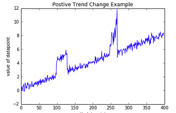
Other types of anomalies can be easily spotted in charts or graphics, such as the chart below.
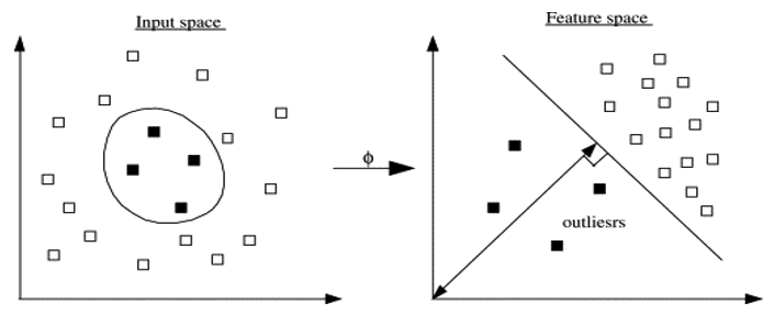 There are many different algorithms available for anomaly detection, and the Oracle Database already has an algorithm called the One-Class Support Vector Machine. This is a variant of the main Support Vector Machine (SVD) algorithm, which maps or transforms the data, using a Kernel function, into space such that the data belonging to the class values are transformed by different amounts. This creates a Hyperplane between the mapped/transformed values and hopefully gives a large margin between the mapped/transformed points. This is what makes SVD very accurate, although it does have some scaling limitations. For a One-Class SVD, a similar process is followed. The aim is for anomalous data to be mapped differently to common or non-anomalous data, as shown in the following diagram.
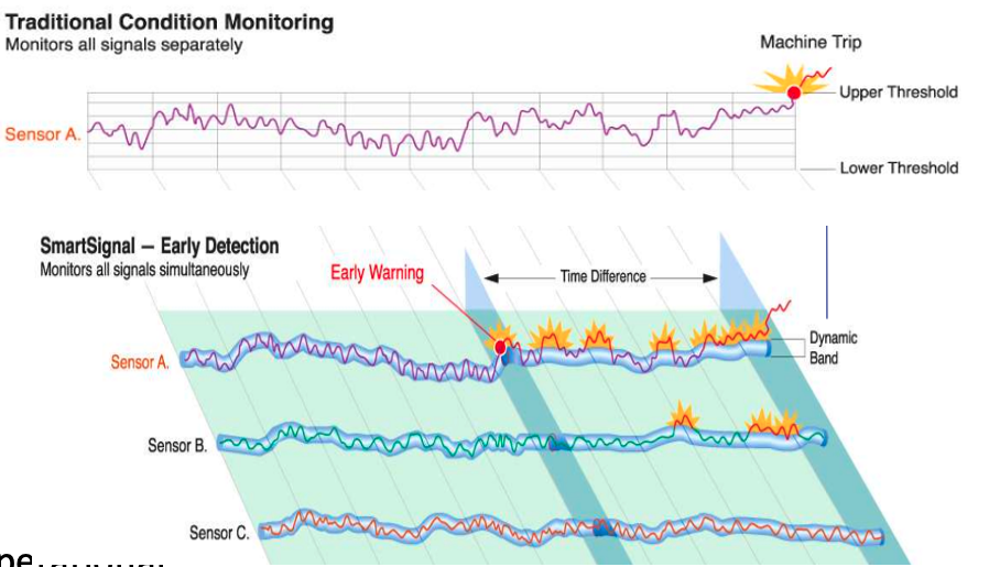
Getting back to the MSET algorithm. Remember it is a 2-part algorithm abbreviated to MSET. The first part is a non-linear, nonparametric anomaly detection algorithm that calibrates the expected behavior of a system based on historical data from the normal sequence of monitored signals. Using data in time series format (DATE, Value) the training data set contains data consisting of “normal” behavior of the data. The algorithm creates a model to represent this “normal”/stationary data/behavior. The second part of the algorithm compares new or live data and calculates the differences between the estimated and actual signal values (residuals). It uses Sequential Probability Ratio Test (SPRT) calculations to determine whether any of the signals have become degraded. As you can imagine the creation of the training data set is vital and may consist of many iterations before determining the optimal training data set to use.
MSET has its origins in computer hardware failures monitoring. Sun Microsystems have been were using it back in the late 1990’s-early 2000’s to monitor and detect for component failures in their servers. Since then MSET has been widely used in power generation plants, airplanes, space travel, Disney uses it for equipment failures, and in more recent times has been extensively used in IOT environments with the anomaly detection focused on signal anomalies.
How does MSET work in Oracle 21c?
An important point to note before we start is, you can use MSET on your typical business data and other data stored in the database. It isn’t just for sensor, IOT, etc data mentioned above and can be used in many different business scenarios.
The first step you need to do is to create the time series data. This can be easily done using a view, but a Very important component is the Time attribute needs to be a DATE format. Additional attributes can be numeric data and these will be used as input to the algorithm for model creation.
-- Create training data set for MSET
CREATE OR REPLACE VIEW mset_train_data
AS SELECT time_id,
          sum(quantity_sold) quantity,
          sum(amount_sold) amount
FROM (SELECT * FROM sh.sales WHERE time_id <= '30-DEC-99’)
GROUP BY time_id
ORDER BY time_id;
The example code above uses the SH schema data, and aggregates the data based on the TIME_ID attribute. This attribute is a DATE data type. The second import part of preparing and formatting the data is Ordering of the data. The ORDER BY is necessary to ensure the data is fed into or processed by the algorithm in the correct time series order.
The next step involves defining the parameters/hyper-parameters for the algorithm. All algorithms come with a set of default values, and in most cases these are suffice for your needs. In that case, you only need to define the Algorithm Name and to turn on Automatic Data Preparation. The following example illustrates this and also includes examples of setting some of the typical parameters for the algorithm.
BEGIN
  DELETE FROM mset_settings;

  -- Select MSET-SPRT as the algorithm
  INSERT  INTO mset_sh_settings (setting_name, setting_value)
  VALUES(dbms_data_mining.algo_name, dbms_data_mining.algo_mset_sprt);

  -- Turn on automatic data preparation
  INSERT INTO mset_sh_settings (setting_name, setting_value)
  VALUES(dbms_data_mining.prep_auto, dbms_data_mining.prep_auto_on);

  -- Set alert count
  INSERT INTO mset_sh_settings (setting_name, setting_value)
  VALUES(dbms_data_mining.MSET_ALERT_COUNT, 3);

  -- Set alert window
  INSERT INTO mset_sh_settings (setting_name, setting_value)
  VALUES(dbms_data_mining.MSET_ALERT_WINDOW, 5);

  -- Set alpha
  INSERT INTO mset_sh_settings (setting_name, setting_value)
  VALUES(dbms_data_mining.MSET_ALPHA_PROB, 0.1);

  COMMIT;
END;
To create the MSET model using the MST_TRAIN_DATA view created above, we can run:
BEGIN
--   DBMS_DATA_MINING.DROP_MODEL(MSET_MODEL');

   DBMS_DATA_MINING.CREATE_MODEL (
      model_name          => 'MSET_MODEL',
      mining_function     => dbms_data_mining.classification,
      data_table_name     => 'MSET_TRAIN_DATA',
      case_id_column_name => 'TIME_ID',
      target_column_name  => '',
      settings_table_name => 'MSET_SETTINGS');
END;
The SELECT statement below is an example of how to call and run the MSET model to label the data to find anomalies. The PREDICTION function will return a values of 0 (zero) or 1 (one) to indicate the predicted values. If the predicted values is 0 (zero) the MSET model has predicted the input record to be anomalous, where as a predicted values of 1 (one) indicates the value is typical. This can be used to filter out the records/data you will want to investigate in more detail.
-- display all dates with Anomalies
SELECT time_id, pred
FROM (SELECT time_id, prediction(mset_sh_model using *) over (ORDER BY time_id) pred
      FROM mset_test_data)
WHERE pred = 0;
