
Machine Learning
Machine Learning App Migration to Oracle Cloud VM
Over the past few years, I’ve been developing a Stock Market prediction algorithm and made some critical refinements to it earlier this year. As with all analytics, data science, machine learning and AI projects, testing is vital to ensure its performance, accuracy and sustainability. Taking such a project out of a lab environment and putting it into a production setting introduces all sorts of different challenges. Some of these challenges include being able to self-manage its own process, logging, traceability, error and event management, etc. Automation is key and implementing all of these extra requirements tasks way more code and time than developing the actual algorithm. Typically, the machine learning and algorithms code only accounts for less than five percent of the actual code, and in some cases, it can be less than one percent!
I’ve come to the stage of deploying my App to a production-type environment, as I’ve been running it from my laptop and then a desktop for over a year now. It’s now 100% self-managing so it’s time to deploy. The environment I’ve chosen is using one of the Virtual Machines (VM) available on the Oracle Free Tier. This means it won’t cost me a cent (dollar or more) to run my App 24×7.
My App has three different components which use a core underlying machine learning predictions engine. Each is focused on a different set of stock markets. These marks operate in the different timezone of US markets, European Markets and Asian Markets. Each will run on a slightly different schedule than the rest.
The steps outlined below take you through what I had to do to get my App up and running the VM (Oracle Free Tier). It took about 20 minutes to complete everything
The first thing you need to do is create a ssh key file. There are a number of ways of doing this and the following is an example.
ssh-keygen -t rsa -N "" -b 2048 -C "myOracleCloudkey" -f myOracleCloudkey
This key file will be used during the creation of the VM and for logging into the VM.
Log into your Oracle Cloud account and you’ll find the Create Instances Compute i.e. create a virtual machine/

Complete the Create Instance form and upload the ssh file you created earlier. Then click the Create button. This assumes you have networking already created.

It will take a minute or two for the VM to be created and you can monitor the progress.
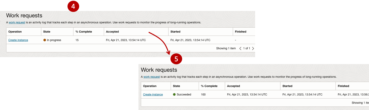
After it has been created you need to click on the start button to start the VM.
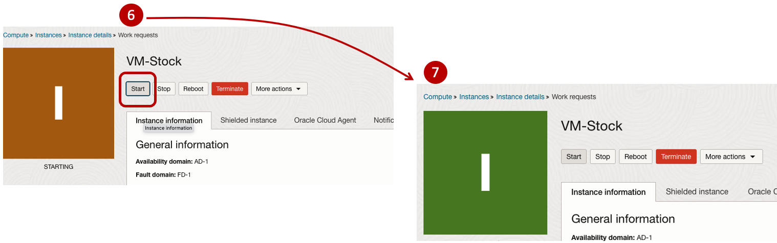
After it has started you can now log into the VM from a terminal window, using the public IP address
ssh -i myOracleCloudKey opc@xxx.xxx.xxx.xxxAfter you’ve logged into the VM it’s a good idea to run an update.
[opc@vm-stocks ~]$ sudo yum -y update
Last metadata expiration check: 0:13:53 ago on Fri 21 Apr 2023 14:39:59 GMT.
Dependencies resolved.
========================================================================================================================
 Package                         Arch       Version                                          Repository            Size
========================================================================================================================
Installing:
 kernel-uek                      aarch64    5.15.0-100.96.32.el8uek                          ol8_UEKR7            1.4 M
 kernel-uek-core                 aarch64    5.15.0-100.96.32.el8uek                          ol8_UEKR7             47 M
 kernel-uek-devel                aarch64    5.15.0-100.96.32.el8uek                          ol8_UEKR7             19 M
 kernel-uek-modules              aarch64    5.15.0-100.96.32.el8uek                          ol8_UEKR7             59 M
Upgrading:
 NetworkManager                  aarch64    1:1.40.0-6.0.1.el8_7                             ol8_baseos_latest    2.1 M
 NetworkManager-config-server    noarch     1:1.40.0-6.0.1.el8_7                             ol8_baseos_latest    141 k
 NetworkManager-libnm            aarch64    1:1.40.0-6.0.1.el8_7                             ol8_baseos_latest    1.9 M
 NetworkManager-team             aarch64    1:1.40.0-6.0.1.el8_7                             ol8_baseos_latest    156 k
 NetworkManager-tui              aarch64    1:1.40.0-6.0.1.el8_7                             ol8_baseos_latest    339 k
...
...
The VM is now ready to setup and install my App. The first step is to install Python, as all my code is written in Python.
[opc@vm-stocks ~]$ sudo yum install -y python39
Last metadata expiration check: 0:20:35 ago on Fri 21 Apr 2023 14:39:59 GMT.
Dependencies resolved.
========================================================================================================================
 Package                         Architecture  Version                                        Repository           Size
========================================================================================================================
Installing:
 python39                        aarch64       3.9.13-2.module+el8.7.0+20879+a85b87b0         ol8_appstream        33 k
Installing dependencies:
 python39-libs                   aarch64       3.9.13-2.module+el8.7.0+20879+a85b87b0         ol8_appstream       8.1 M
 python39-pip-wheel              noarch        20.2.4-7.module+el8.6.0+20625+ee813db2         ol8_appstream       1.1 M
 python39-setuptools-wheel       noarch        50.3.2-4.module+el8.5.0+20364+c7fe1181         ol8_appstream       497 k
Installing weak dependencies:
 python39-pip                    noarch        20.2.4-7.module+el8.6.0+20625+ee813db2         ol8_appstream       1.9 M
 python39-setuptools             noarch        50.3.2-4.module+el8.5.0+20364+c7fe1181         ol8_appstream       871 k
Enabling module streams:
 python39                                      3.9

Transaction Summary
========================================================================================================================
Install  6 Packages

Total download size: 12 M
Installed size: 47 M
Downloading Packages:
(1/6): python39-pip-20.2.4-7.module+el8.6.0+20625+ee813db2.noarch.rpm                    23 MB/s | 1.9 MB     00:00
(2/6): python39-pip-wheel-20.2.4-7.module+el8.6.0+20625+ee813db2.noarch.rpm             5.5 MB/s | 1.1 MB     00:00
...
...
Next copy the code to the VM, setup the environment variables and create any necessary directories required for logging. The final part of this is to download the connection Wallett for the Database. I’m using the Python library oracledb, as this requires no additional setup.
Then install all the necessary Python libraries used in the code, for example, pandas, matplotlib, tabulate, seaborn, telegram, etc (this is just a subset of what I needed). For example here is the command to install pandas.
pip3.9 install pandasAfter all of that, it’s time to test the setup to make sure everything runs correctly.
The final step is to schedule the App/Code to run. Before setting the schedule just do a quick test to see what timezone the VM is running with. Run the date command and you can see what it is. In my case, the VM is running GMT which based on the current time locally, the VM was showing to be one hour off. Allowing for this adjustment and for day-light saving time, the time +/- markets openings can be set. The following example illustrates setting up crontab to run the App, Monday-Friday, between 13:00-22:00 and at 5-minute intervals. Open crontab and edit the schedule and command. The following is an example
> contab -e

*/5 13-22 * * 1-5 python3.9 /home/opc/Stocks.py >Stocks.txt
For some stock market trading apps, you might want it to run more frequently (than every 5 minutes) or less frequently depending on your strategy.
After scheduling the components for each of the Geographic Stock Market areas, the instant messaging of trades started to appear within a couple of minutes. After a little monitoring and validation checking, it was clear everything was running as expected. It was time to sit back and relax and see how this adventure unfolds.
For anyone interested, the App does automated trading with different brokers across the markets, while logging all events and trades to an Oracle Autonomous Database (Free Tier = no cost), and sends instant messages to me notifying me of the automated trades. All I have to do is Nothing, yes Nothing, only to monitor the trade notifications. I mentioned earlier the importance of testing, and with back-testing of the recent changes/improvements (as of the date of post), the App has given a minimum of 84% annual return each year for the past 15 years. Most years the return has been a lot more!
Image Augmentation (Pencil & Cartoon) with OpenCV #SYM42
OpenCV has been with us for over two decades and provides us with a rich open-source library for performing image processing.
In this post I’m going to illustrate how you can use it to convert images (of people) into pencil sketches and cartoon images. As with most examples you find on such technologies there are things it is good at and some things this isn’t good at. Using the typical IT phrase, “It Depends” comes into play with image processing. What might work with one set of images, might not work as well with others.
The example images below consist of the Board of a group called SYM42, or Symposium42. Yes, they said I could use their images and show the output from using OpenCV 🙂 This group was formed by a community to support the community, was born out of an Oracle Community but is now supporting other technologies. They are completely independent of any Vendor which means they can be 100% honest about which aspects of any product do or do not work and are not influenced by the current sales or marketing direction of any company. Check out their About page.
Let’s get started. After downloading the images to process, let’s view them.
import cv2
import matplotlib.pyplot as plt
import numpy as np

dir = '/Users/brendan.tierney/Dropbox/6-Screen-Background/'
file = 'SYM42-Board-Martin.jpg'

image = cv2.imread(dir+file)
img_name = 'Original Image'
#Show the image with matplotlib
#plt.imshow(image)

#OpenCV uses BGR color scheme whereas matplotlib uses RGB colors scheme
#convert BGR image to RGB by using the following
plt.imshow(cv2.cvtColor(image, cv2.COLOR_BGR2RGB))
plt.axis(False)
plt.show()

I’m using Jupyter Notebooks for this work. In the above code, you’ll see I’ve commented out the line [#plt.imshow(image)]. This comment doesn’t really work in Jupyter Notebooks and instead you need to swap to using Matplotlib to display the images
To convert to a pencil sketch, we need to convert to pencil sketch, apply a Gaussian Blur, invert the image and perform bit-wise division to get the final pencil sketch.
#convert to grey scale
#cvtColor function
grey_image = cv2.cvtColor(image, cv2.COLOR_BGR2GRAY)
#invert the image
invert_image = cv2.bitwise_not(grey_image)

#apply Gaussian Blue : adjust values until you get pencilling effect required
blur_image=cv2.GaussianBlur(invert_image, (21,21),0)  #111,111

#Invert Blurred Image
#Repeat previous step
invblur_image=cv2.bitwise_not(blur_image)

#The sketch can be obtained by performing bit-wise division between
# the grayscale image and the inverted-blurred image.
sketch_image=cv2.divide(grey_image, invblur_image, scale=256.0)

#display the pencil sketch
plt.imshow(cv2.cvtColor(sketch_image, cv2.COLOR_BGR2RGB))
plt.axis(False)
plt.show()
The following code listing contains the same as above and also includes the code to convert to a cartoon style.
import os
import glob
import cv2
import matplotlib.pyplot as plt
import numpy as np

def edge_mask(img, line_size, blur_value):
  gray = cv2.cvtColor(img, cv2.COLOR_BGR2GRAY)
  gray_blur = cv2.medianBlur(gray, blur_value)
  edges = cv2.adaptiveThreshold(gray_blur, 255, cv2.ADAPTIVE_THRESH_MEAN_C, cv2.THRESH_BINARY, line_size, blur_value)
  return edges

def cartoon_image(img_cartoon):
    img=img_cartoon

    line_size = 7
    blur_value = 7
    edges = edge_mask(img, line_size, blur_value)

    #Clustering - (K-MEANS)
    imgf=np.float32(img).reshape(-1,3)
    criteria=(cv2.TERM_CRITERIA_EPS+cv2.TERM_CRITERIA_MAX_ITER,20,1.0)
    compactness,label,center=cv2.kmeans(imgf,5,None,criteria,10,cv2.KMEANS_RANDOM_CENTERS)
    center=np.uint8(center)
    final_img=center[label.flatten()]
    final_img=final_img.reshape(img.shape)

    cartoon=cv2.bitwise_and(final_img,final_img,mask=edges)

    return cartoon

def sketch_image(image_file, blur):
    import_image = cv2.imread(image_file)

    #cvtColor function
    grey_image = cv2.cvtColor(import_image, cv2.COLOR_BGR2GRAY)
    #invert the image
    invert_image = cv2.bitwise_not(grey_image)

    blur_image=cv2.GaussianBlur(invert_image, (blur,blur),0)   #111,111

    #Invert Blurred Image
    #Repeat previous step
    invblur_image=cv2.bitwise_not(blur_image)

    sketch_image=cv2.divide(grey_image, invblur_image, scale=256.0)
    cartoon_img=cartoon_image(import_image)

    #plot images
#    plt.figure(figsize=(9,6))
    plt.rcParams["figure.figsize"] = (12,8)

    #plot cartoon
    plt.subplot(1,3,3)
    plt.imshow(cv2.cvtColor(cartoon_img, cv2.COLOR_BGR2RGB))
    plt.title('Cartoon Image', size=12, color='red')
    plt.axis(False)

    #plot sketch
    plt.subplot(1,3,2)
    plt.imshow(cv2.cvtColor(sketch_image, cv2.COLOR_BGR2RGB))
    plt.title('Sketch Image', size=12, color='red')
    plt.axis(False)
    #plot original image
    plt.subplot(1,3,1)
    plt.imshow(cv2.cvtColor(import_image, cv2.COLOR_BGR2RGB))
    plt.title('Original Image', size=12, color='blue')
    plt.axis(False)

    #plot show
    plt.show()

for filepath in glob.iglob(dir+'SYM42-Board*.*'):
    #print(filepath)
    #import_image = cv2.imread(dir+file)
    sketch_image(filepath, 23)
For the SYM42 Board members, we get the following output.

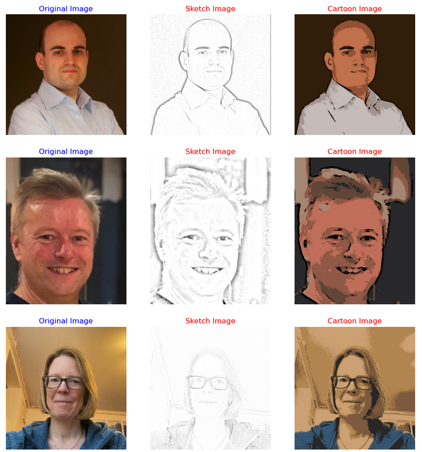
As you can see from these images, some are converted in a way you would expect. While others seem to give little effect.
Thanks to the Board of SYM42 for allowing me to use their images.
AutoML using Pycaret
In this post we will have a look at using the AutoML feature in the Pycaret Python library. AutoML is a popular topic and allows Data Scientists and Machine Learning people to develop potentially optimized models based on their data. All requiring the minimum of input from the Data Scientist. As with all AutoML solutions, care is needed on the eventual use of these models. With various ML and AI Legal requirements around the World, it might not be possible to use the output from AutoML in production. But instead, gives the Data Scientists guidance on creating an optimized model, which can then be deployed in production. This facilitates requirements around model explainability, transparency, human oversight, fairness, risk mitigation and human in the loop.
Some useful links
Pycaret as all your typical Machine Learning algorithms and functions, including for classification, regression, clustering, anomaly detection, time series analysis, and so on.
To install Pycaret run the typical pip command
pip3 install pycaret
If you get any error messages when running any of the following example code, you might need to have a look at your certificates. Locate where Python is installed (for me on a Mac /Applications/Python 3.7) and you will find a command called ‘Install Certificates.command’. and run the following in the Python directory. This should fix what is causing the errors.
Pycaret comes with some datasets. Most of these are the typical introduction datasets you will find in other Python libraries and in various dataset repositories. For our example we are going to use the Customer Credit dataset. This contains data for a classification problem and the aim is to predict customers who are likely to default.
Let’s load the data and have a quick explore
#Don't forget to install Pycaret
#pip3 install pycaret

#Import dataset from Pycaret
from pycaret.datasets import get_data

#Credit defaulters dataset
df = get_data("credit")
The dataframe is displayed for the first five records
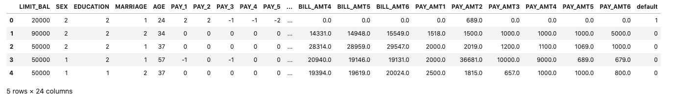
What’s the shape of the dataframe? The dataset/frame has 24,000 records and 24 columns.
#Check for the shape of the dataset
df.shape

(24000, 24)
The dataset has been formatted for a Classification problem with the column ‘default’ being the target or response variable. Let’s have a look at the distribution of records across each value in the ‘default’ column.
df['default'].value_counts()

0    18694
1     5306
And to get the percentage of these distributions,
df['default'].value_counts(normalize=True)*100

0    77.891667
1    22.108333
Before we can call the AutoML function, we need to create our Training and Test datasets.
#Initialize seed for random generators and reproducibility
seed = 42

#Create the train set using pandas sampling - seen data set
train = df.sample(frac=.8, random_state=seed)
train.reset_index(inplace=True, drop=True)
print(train.shape)
train['default'].value_counts()

(19200, 24)

0    14992
1     4208
Now the Test dataset.
#Using samples not available in train as future or unseen data set
test = df.drop(train.index)
test.reset_index(inplace=True, drop=True)
print(test.shape)
test['default'].value_counts()

(4800, 24)

0    3798
1    1002
Next we need to setup and configure the AutoML experiment.
#Let's Do some magic!
from pycaret.classification import *

#Setup function initializes the environment and creates the transformation pipeline
clf = setup(data=train, target="default", session_id=42)
When the above is run, it goes through a number of steps. The first looks at the dataset, the columns and determines the data types, displaying the following.

If everything is correct, press the enter key to confirm the datatypes, otherwise type ‘quit‘. If you press enter Pycaret will complete the setup of the experiments it will perform to identify a model. A subset of the 60 settings is shown below.

The next step runs the experiments to compare each of the models (AutoML), evaluates them and then prints out a league table of models with values for various model evaluation measures. 5.-Fold cross validation is used for each model. This league table is updated are each model is created and evaluated.
# Compares different models depending on their performance metrics. By default sorted by accuracy
best_model = compare_models(fold=5)
For this dataset, this process of comparing the models (AutoML) only takes a few seconds. The constant updating of the league tables is a nice touch. The following shows the final league table created for our AutoML.

The cells colored/highlighted in Yellow tells you which model scored based for that particular evaluation matrix. Here we can see Ridge Classifier scored best using Accuracy and Precision. While the Linear Discriminant Analysis model was best using F1 score, Kappa and MCC.
print(best_model)

RidgeClassifier(alpha=1.0, class_weight=None, copy_X=True, fit_intercept=True,
                max_iter=None, normalize=False, random_state=42, solver='auto',
                tol=0.001)
We can also print the ROC chart.
# Plots the AUC curve
import matplotlib.pyplot as plt

fig = plt.figure()
plt.figure(figsize = (14,10))
plot_model(best_model, plot="auc", scale=1)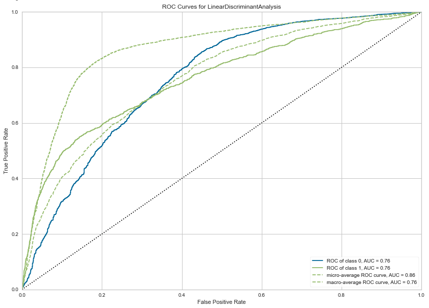
Also the confusion matrix.
plot_model(best_model, plot="confusion_matrix")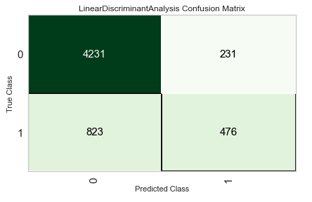
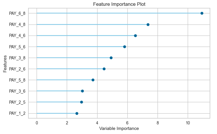
We can also see what the top features are that contribute to the model outcomes (the predictions). This is also referred to as feature importance.
plot_model(best_model, plot="feature")
We could take one of these particular models and tune it for a better fit, or we could select the ‘best’ model and tune it.
# Tune model function performs a grid search to identify the best parameters
tuned = tune_model(best_model)
We can now use the tuned model to label the Test dataset and compare the results.
# Predict on holdout set
predict_model(tuned, data=test)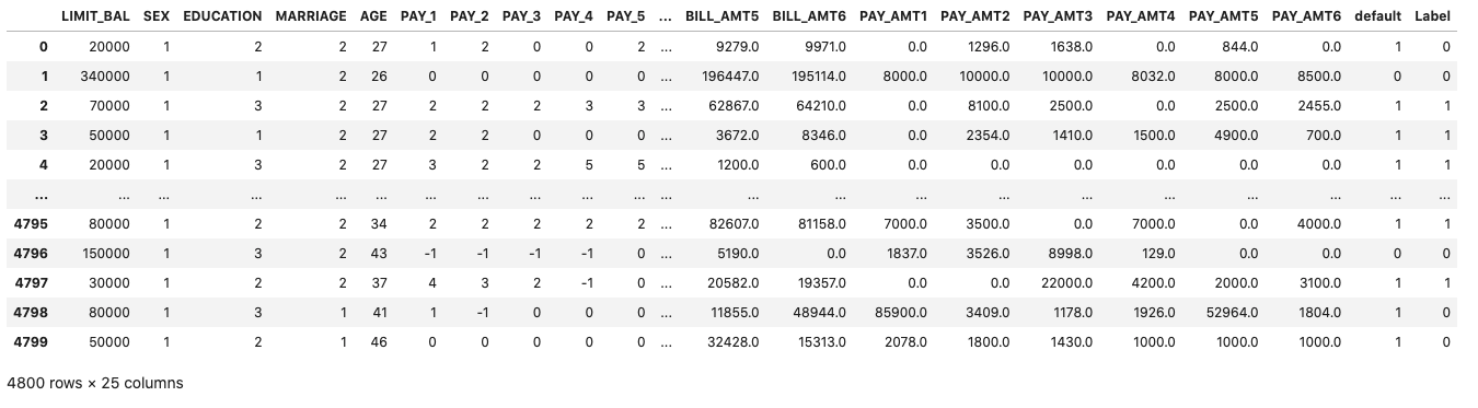
The final steps with all models is to save it for later use. Pycaret allows you to save the model in .pkl file format
# Model will be saved as .pkl and can be utilized for serving
save_model(tuned,'Tuned-Model-AutoML-Pycaret')
That’s it. All done.
Combining NLP and Machine Learning for Document Classification
Text mining is a popular topic for exploring what text you have in documents etc. Text mining and NLP can help you discover different patterns in the text like uncovering certain words or phases which are commonly used, to identifying certain patterns and linkages between different texts/documents. Combining this work on Text mining you can use Word Clouds, time-series analysis, etc to discover other aspects and patterns in the text. Check out my previous blog posts (post 1, post 2) on performing Text Mining on documents (manifestos from some of the political parties from the last two national government elections in Ireland). These two posts gives you a simple indication of what is possible.
We can build upon these Text Mining examples to include other machine learning algorithms like those for Classification. With Classification we want to predict or label a record or document to have a particular value. With Classification this could involve labeling a document as being positive or negative (movie or book reviews), or determining if a document is for a particular domain such as Technology, Sports, Entertainment, etc
With Classification problems we typically have a case record containing many different feature/attributes. You will see many different examples of this. When we add in Text Mining we are adding new/additional features/attributes to the case record. These new features/attributes contain some characteristics of the Word (or Term) frequencies in the documents. This is a form of feature engineering, where we create new features/attributes based on our dataset.
Let’s work through an example of using Text Mining and Classification Algorithm to build a model for determining/labeling/classifying documents.
The Dataset: For this example I’ll use Move Review dataset from Cornell University. Download and unzip the file. This will create a set of directories with the reviews (as individual documents) listed under the ‘pos’ or ‘neg’ directory. This dataset contains approximately 2000 documents. Other datasets you could use include the Amazon Reviews or the Disaster Tweets.
The following is the Python code to perform NLP to prepare the data, build a classification model and test this model against a holdout dataset. First thing is to load the libraries NLP and some other basics.
import numpy as np
import re
import nltk
from sklearn.datasets import load_files
from nltk.corpus import stopwords
Load the dataset.
#This dataset will allow use to perform a type of Sentiment Analysis Classification
source_file_dir = r"/Users/brendan.tierney/Dropbox/4-Datasets/review_polarity/txt_sentoken"

#The load_files function automatically divides the dataset into data and target sets.
#load_files  will treat each folder inside the "txt_sentoken" folder as one category
#  and all the documents inside that folder will be assigned its corresponding category.
movie_data = load_files(source_file_dir)
X, y = movie_data.data, movie_data.target

#load_files  function loads the data from both "neg" and "pos" folders into the X variable,
#  while the target categories are stored in y
We can now use the typical NLP tasks on this data. This will clean the data and prepare it.
documents = []
documents = []

from nltk.stem import WordNetLemmatizer

stemmer = WordNetLemmatizer()

for sen in range(0, len(X)):
    # Remove all the special characters, numbers, punctuation
    document = re.sub(r'\W', ' ', str(X[sen]))

    # remove all single characters
    document = re.sub(r'\s+[a-zA-Z]\s+', ' ', document)

    # Remove single characters from the start of document with a space
    document = re.sub(r'\^[a-zA-Z]\s+', ' ', document)

    # Substituting multiple spaces with single space
    document = re.sub(r'\s+', ' ', document, flags=re.I)

    # Removing prefixed 'b'
    document = re.sub(r'^b\s+', '', document)

    # Converting to Lowercase
    document = document.lower()

    # Lemmatization
    document = document.split()

    document = [stemmer.lemmatize(word) for word in document]
    document = ' '.join(document)

    documents.append(document)
You can see we have removed all special characters, numbers, punctuation, single characters, spacing, special prefixes, converted all words to lower case and finally extracted the stemmed word.
Next we need to take these words and convert them into numbers, as the algorithms like to work with numbers rather then text. One particular approach is Bag of Words.
The first thing we need to decide on is the maximum number of words/features to include or use for later stages. As you can image when looking across lots and lots of documents you will have a very large number of words. Some of these are repeated words. What we are interested in are frequently occurring words, which means we can ignore low frequently occurring works. To do this we can set max_feature to a defined value. In our example we will set it to 1500, but in your problems/use cases you might need to experiment to determine what might be a better values.
Two other parameters we need to set include min_df and max_df. min_df sets the minimum number of documents to contain the word/feature. max_df specifies the percentage of documents where the words occur, for example if this is set to 0.7 this means the words should occur in a maximum of 70% of the documents.
from sklearn.feature_extraction.text import CountVectorizer
vectorizer = CountVectorizer(max_features=1500, min_df=5, max_df=0.7,stop_words=stopwords.words('english'))
X = vectorizer.fit_transform(documents).toarray()
The CountVectorizer in the above code also remove Stop Words for the English language. These words are generally basic words that do not convey any meaning. You can easily add to this list and adjust it to suit your needs and to reflect word usage and meaning for your particular domain.
The bag of words approach works fine for converting text to numbers. However, it has one drawback. It assigns a score to a word based on its occurrence in a particular document. It doesn’t take into account the fact that the word might also be having a high frequency of occurrence in other documentsas well. TFIDF resolves this issue by multiplying the term frequency of a word by the inverse document frequency. The TF stands for “Term Frequency” while IDF stands for “Inverse Document Frequency”.
And the Inverse Document Frequency is calculated as:
IDF(word) = Log((Total number of documents)/(Number of documents containing the word))
The term frequency is calculated as:
Term frequency = (Number of Occurrences of a word)/(Total words in the document)
The TFIDF value for a word in a particular document is higher if the frequency of occurrence of thatword is higher in that specific document but lower in all the other documents.
To convert values obtained using the bag of words model into TFIDF values, run the following:
from sklearn.feature_extraction.text import TfidfTransformer
tfidfconverter = TfidfTransformer()
X = tfidfconverter.fit_transform(X).toarray()
That’s the dataset prepared, the final step is to create the Training and Test datasets.
from sklearn.model_selection import train_test_split
X_train, X_test, y_train, y_test = train_test_split(X, y, test_size=0.2, random_state=0)
#Train DS = 70%
#Test DS = 30%
There are several machine learning algorithms you can use. These are the typical classification algorithms. But for simplicity I’m going to use RandomForest algorithm in the following code. After giving this a go, try to do it for the other algorithms and compare the results.
#Import Random Forest Model
#Use RandomForest algorithm to create a model
#n_estimators = number of trees in the Forest

from sklearn.ensemble import RandomForestClassifier
classifier = RandomForestClassifier(n_estimators=1000, random_state=0)
classifier.fit(X_train, y_train)
Now we can test the model on the hold-out or Test dataset
#Now label/classify the Test DS
y_pred = classifier.predict(X_test)

#Evaluate the model
from sklearn.metrics import classification_report, confusion_matrix, accuracy_score

print("Accuracy:", accuracy_score(y_test, y_pred))
print(confusion_matrix(y_test,y_pred))
print(classification_report(y_test,y_pred))
This model gives the following results, with an over all accuracy of 85% (you might get a slightly different figure). This is a good outcome and a good predictive model. But is it the best one? We simply don’t know at this point. Using the ‘No Free Lunch Theorem’ we would would have to see what results we would get from the other algorithms.
Although this example only contains the words from the documents, we can see how we could include this with other features/attributes when forming a case record. For example, our case records represented Insurance Claims, the features would include details of the customer, their insurance policy, the amount claimed, etc and in addition could include incident reports, claims assessor reports etc. This would be documents which we can include in the building a predictive model to determine of an insurance claim is fraudulent or not.
Comparing Cluster Algorithms on Density Data
In a previous posted I gave a detailed description of using DBScan to create clusters for a dataset containing different density based data. This “manufactured” dataset was created to illustrate how and why DBScan can be used.
But taking the previous post in isolation is perhaps not recommended. As a Data Scientist you will need to use many Clustering algorithms to determine which algorithm can best identify the patterns in your data, and this can be determined by the type of data distributions within the dataset.
The DBScan post created the following diagrams. The diagram on the left is a plot of the dataset where we can easily identify different groupings/clusters. The diagram on the right illustrates the clusters identified by DBScan. As you can see it did a good job.
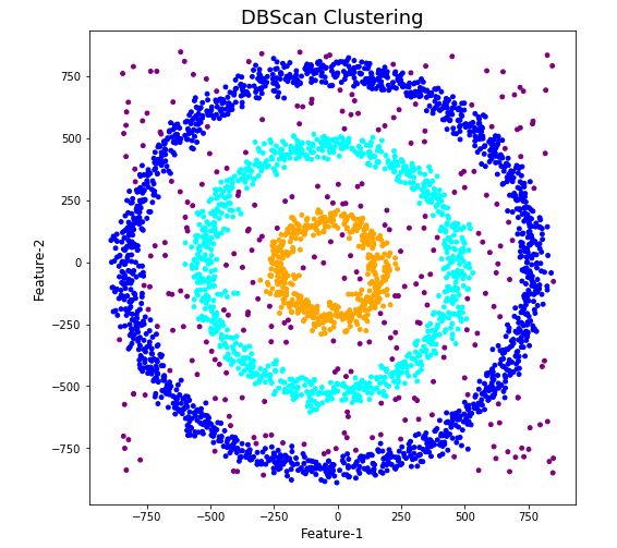
We can see the three clusters and the noisy data point which were added to the dataset.
But what about other Clustering algorithms? What about k-Means and Hierarchical Clustering algorithms? How would they perform on this dataset?
Here is the code for k-Means with three clusters. Three clusters was selected as we have three clear clusters in the dataset.
#k-Means with 3 clusters
from sklearn.cluster import KMeans
k_means=KMeans(n_clusters=3,random_state=42)
k_means.fit(df[[0,1]])

df['KMeans_labels']=k_means.labels_

# Plotting resulting clusters
colors=['purple','red','blue','green']
plt.figure(figsize=(10,10))
plt.scatter(df[0],df[1],c=df['KMeans_labels'],cmap=matplotlib.colors.ListedColormap(colors),s=15)
plt.title('K-Means Clustering',fontsize=18)
plt.xlabel('Feature-1',fontsize=12)
plt.ylabel('Feature-2',fontsize=12)
plt.show()
Here is the code for Hierarchical Clustering, again three clusters was selected.
from sklearn.cluster import AgglomerativeClustering
model = AgglomerativeClustering(n_clusters=3, affinity='euclidean')
model.fit(df[[0,1]])

df['HR_labels']=model.labels_

# Plotting resulting clusters
plt.figure(figsize=(10,10))
plt.scatter(df[0],df[1],c=df['HR_labels'],cmap=matplotlib.colors.ListedColormap(colors),s=15)
plt.title('Hierarchical Clustering',fontsize=20)
plt.xlabel('Feature-1',fontsize=14)
plt.ylabel('Feature-2',fontsize=14)
plt.show()
The diagrams from both of these are shown below.
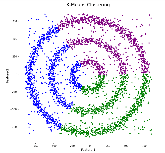
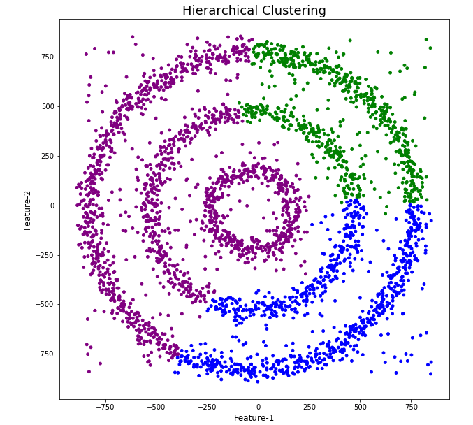
As you can see the results generated by these alternative Clustering algorithms produce very different results to what was produced by DBScan (see image at top of post) and we can easily see which algorithm best fits the dataset used.
Make sure you check out the post on DBScan.
DBScan Clustering in Python
Unsupervised Learning is a common approach for discovering patterns in datasets. The main algorithmic approach in Unsupervised Learning is Clustering, where the data is searched to discover groupings, or clusters, of data. Each of these clusters contain data points which have some set of characteristics in common with each other, and each cluster is distinct and different. There are many challenges with clustering which include trying to interpret the meaning of each cluster and how it is related to the domain in question, what is the “best” number of clusters to use or have, the shape of each cluster can be different (not like the nice clean examples we see in the text books), clusters can be overlapping with a data point belonging to many different clusters, and the difficulty with trying to decide which clustering algorithm to use.
The last point above about which clustering algorithm to use is similar to most problems in Data Science and Machine Learning. The simple answer is we just don’t know, and this is where the phases of “No free lunch” and “All models are wrong, but some models are model that others”, apply. This is where we need to apply the various algorithms to our data, and through a deep process of investigation the outputs, of each algorithm, need to be investigated to determine what algorithm, the parameters, etc work best for our dataset, specific problem being investigated and the domain. This involve the needs for lots of experiments and analysis. This work can take some/a lot of time to complete.
The k-Means clustering algorithm gets a lot of attention and focus for Clustering. It’s easy to understand what it does and to interpret the outputs. But it isn’t perfect and may not describe your data, as it can have different characteristics including shape, densities, sparseness, etc. k-Means focuses on a distance measure, while algorithms like DBScan can look at the relative densities of data. These two different approaches can produce by different results. Careful analysis of the data and the results/outcomes of these algorithms needs some care.
Let’s illustrate the use of DBScan (Density Based Spatial Clustering of Applications with Noise), using the scikit-learn Python package, for a “manufactured” dataset. This example will illustrate how this density based algorithm works (See my other blog post which compares different Clustering algorithms for this same dataset). DBSCAN is better suited for datasets that have disproportional cluster sizes (or densities), and whose data can be separated in a non-linear fashion.
There are two key parameters of DBScan:
- eps: The distance that specifies the neighborhoods. Two points are considered to be neighbors if the distance between them are less than or equal to eps.
- minPts: Minimum number of data points to define a cluster.
Based on these two parameters, points are classified as core point, border point, or outlier:
- Core point: A point is a core point if there are at least minPts number of points (including the point itself) in its surrounding area with radius eps.
- Border point: A point is a border point if it is reachable from a core point and there are less than minPts number of points within its surrounding area.
- Outlier: A point is an outlier if it is not a core point and not reachable from any core points.
The algorithm works by randomly selecting a starting point and it’s neighborhood area is determined using radius eps. If there are at least minPts number of points in the neighborhood, the point is marked as core point and a cluster formation starts. If not, the point is marked as noise. Once a cluster formation starts (let’s say cluster A), all the points within the neighborhood of initial point become a part of cluster A. If these new points are also core points, the points that are in the neighborhood of them are also added to cluster A. Next step is to randomly choose another point among the points that have not been visited in the previous steps. Then same procedure applies. This process finishes when all points are visited.
Let’s setup our data set and visualize it.
import numpy as np
import pandas as pd
import math
import matplotlib.pyplot as plt
import matplotlib
#initialize the random seed
np.random.seed(42) #it is the answer to everything!
#Create a function to create our data points in a circular format
#We will call this function below, to create our dataframe
def CreateDataPoints(r, n):
return [(math.cos(2*math.pi/n*x)*r+np.random.normal(-30,30),math.sin(2*math.pi/n*x)*r+np.random.normal(-30,30)) for x in range(1,n+1)]
#Use the function to create different sets of data, each having a circular format
df=pd.DataFrame(CreateDataPoints(800,1500)) #500, 1000
df=df.append(CreateDataPoints(500,850)) #300, 700
df=df.append(CreateDataPoints(200,450)) #100, 300
# Adding noise to the dataset
df=df.append([(np.random.randint(-850,850),np.random.randint(-850,850)) for i in range(450)])
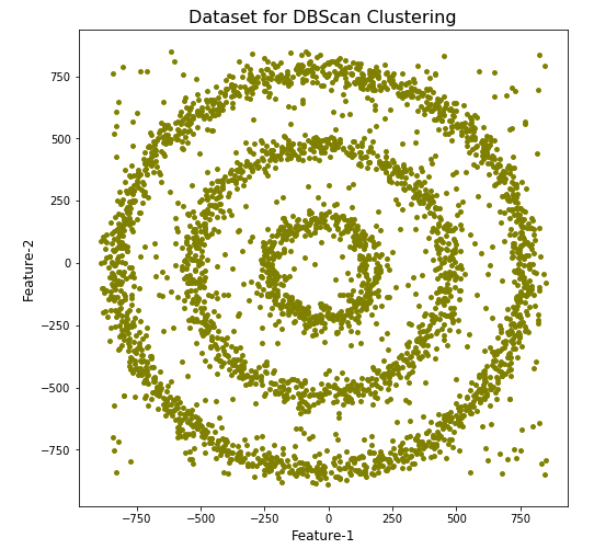
plt.figure(figsize=(8,8))
plt.scatter(df[0],df[1],s=15,color='olive')
plt.title('Dataset for DBScan Clustering',fontsize=16)
plt.xlabel('Feature-1',fontsize=12)
plt.ylabel('Feature-2',fontsize=12)
plt.show()

We can see the dataset we’ve just created has three distinct circular patterns of data. We also added some noisy data too, which can be see as the points between and outside of the circular patterns.
Let’s use the DBScan algorithm, using the default setting, to see what it discovers.
from sklearn.cluster import DBSCAN
#DBSCAN without any parameter optimization and see the results.
dbscan=DBSCAN()
dbscan.fit(df[[0,1]])

df['DBSCAN_labels']=dbscan.labels_

# Plotting resulting clusters
colors=['purple','red','blue','green']
plt.figure(figsize=(8,8))
plt.scatter(df[0],df[1],c=df['DBSCAN_labels'],cmap=matplotlib.colors.ListedColormap(colors),s=15)
plt.title('DBSCAN Clustering',fontsize=16)
plt.xlabel('Feature-1',fontsize=12)
plt.ylabel('Feature-2',fontsize=12)
plt.show()
#Not very useful !
#Everything belongs to one cluster.
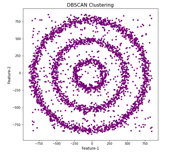
Everything is the one color! which means all data points below to the same cluster. This isn’t very useful and can at first seem like this algorithm doesn’t work for our dataset. But we know it should work given the visual representation of the data. The reason for this occurrence is because the value for epsilon is very small. We need to explore a better value for this. One approach is to use KNN (K-Nearest Neighbors) to calculate the k-distance for the data points and based on this graph we can determine a possible value for epsilon.
#Let's explore the data and work out a better setting
from sklearn.neighbors import NearestNeighbors
neigh = NearestNeighbors(n_neighbors=2)
nbrs = neigh.fit(df[[0,1]])
distances, indices = nbrs.kneighbors(df[[0,1]])

# Plotting K-distance Graph
distances = np.sort(distances, axis=0)
distances = distances[:,1]
plt.figure(figsize=(14,8))
plt.plot(distances)
plt.title('K-Distance - Check where it bends',fontsize=16)
plt.xlabel('Data Points - sorted by Distance',fontsize=12)
plt.ylabel('Epsilon',fontsize=12)
plt.show()
#Let’s plot our K-distance graph and find the value of epsilon

Look at the graph above we can see the main curvature is between 20 and 40. Taking 30 at the mid-point of this we can now use this value for epsilon. The value for the number of samples needs some experimentation to see what gives the best fit.
Let’s now run DBScan to see what we get now.
from sklearn.cluster import DBSCAN
dbscan_opt=DBSCAN(eps=30,min_samples=3)
dbscan_opt.fit(df[[0,1]])

df['DBSCAN_opt_labels']=dbscan_opt.labels_
df['DBSCAN_opt_labels'].value_counts()

# Plotting the resulting clusters
colors=['purple','red','blue','green', 'olive', 'pink', 'cyan', 'orange', 'brown' ]
plt.figure(figsize=(8,8))
plt.scatter(df[0],df[1],c=df['DBSCAN_opt_labels'],cmap=matplotlib.colors.ListedColormap(colors),s=15)
plt.title('DBScan Clustering',fontsize=18)
plt.xlabel('Feature-1',fontsize=12)
plt.ylabel('Feature-2',fontsize=12)
plt.show()

When we look at the dataframe we can see it create many different cluster, beyond the three that we might have been expecting. Most of these clusters contain small numbers of data points. These could be considered outliers and alternative view of this results is presented below, with this removed.
df['DBSCAN_opt_labels']=dbscan_opt.labels_
df['DBSCAN_opt_labels'].value_counts()

 0     1559
 2      898
 3      470
-1      282
 8        6
 5        5
 4        4
 10       4
 11       4
 6        3
 12       3
 1        3
 7        3
 9        3
 13       3
Name: DBSCAN_opt_labels, dtype: int64
The cluster labeled with -1 contains the outliers. Let’s clean this up a little.
df2 = df[df['DBSCAN_opt_labels'].isin([-1,0,2,3])]
df2['DBSCAN_opt_labels'].value_counts()
 0    1559
 2     898
 3     470
-1     282
Name: DBSCAN_opt_labels, dtype: int64

# Plotting the resulting clusters
colors=['purple','red','blue','green', 'olive', 'pink', 'cyan', 'orange']
plt.figure(figsize=(8,8))
plt.scatter(df2[0],df2[1],c=df2['DBSCAN_opt_labels'],cmap=matplotlib.colors.ListedColormap(colors),s=15)
plt.title('DBScan Clustering',fontsize=18)
plt.xlabel('Feature-1',fontsize=12)
plt.ylabel('Feature-2',fontsize=12)
plt.show()

See my other blog post which compares different Clustering algorithms for this same dataset.
Ireland AI Strategy (2021)
Over the past year or more there was been a significant increase in publications, guidelines, regulations/laws and various other intentions relating to these. Artificial Intelligence (AI) has been attracting a lot of attention. Most of this attention has been focused on how to put controls on how AI is used across a wide range of use cases. We have heard and read lots and lots of stories of how AI has been used in questionable and ethical scenarios. These have, to a certain extent, given the use of AI a bit of a bad label. While some of this is justified, some is not, but some allows us to question the ethical use of these technologies. But not all AI, and the underpinning technologies, are bad. Most have been developed for good purposes and as these technologies mature they sometimes get used in scenarios that are less good.
We constantly need to develop new technologies and deploy these in real use scenarios. Ireland has a long history as a leader in the IT industry, with many of the top 100+ IT companies in the world having research and development operations in Ireland, as well as many service suppliers. The Irish government recently released the National AI Strategy (2021).
“The National AI Strategy will serve as a roadmap to an ethical, trustworthy and human-centric design, development, deployment and governance of AI to ensure Ireland can unleash the potential that AI can provide”. “Underpinning our Strategy are three core principles to best embrace the opportunities of AI – adopting a human-centric approach to the application of AI; staying open and adaptable to innovations; and ensuring good governance to build trust and confidence for innovation to flourish, because ultimately if AI is to be truly inclusive and have a positive impact on all of us, we need to be clear on its role in our society and ensure that trust is the ultimate marker of success.” Robert Troy, Minister of State for Trade Promotion, Digital and Company Regulation.
The eight different strands are identified and each sets out how Ireland can be an international leader in using AI to benefit the economy and society.
- Building public trust in AI
- Strand 1: AI and society
- Strand 2: A governance ecosystem that promotes trustworthy AI
- Leveraging AI for economic and societal benefit
- Strand 3: Driving adoption of AI in Irish enterprise
- Strand 4: AI serving the public
- Enablers for AI
- Strand 5: A strong AI innovation ecosystem
- Strand 6: AI education, skills and talent
- Strand 7: A supportive and secure infrastructure for AI
- Strand 8: Implementing the Strategy
Each strand has a clear list of objectives and strategic actions for achieving each strand, at national, EU and at a Global level.
Check out the full document here.

Regulating AI around the World
Continuing my series of blog posts on various ML and AI regulations and laws, this post will look at what some other countries are doing to regulate ML and AI, with a particular focus on facial recognition and more advanced applications of ML. Some of the examples listed below are work-in-progress, while others such as EU AI Regulations are at a more advanced stage with introduction of regulations and laws.
[Note: What is listed below is in addition to various data protection regulations each country or region has implemented in recent years, for example EU GDPR and similar]
Things are moving fast in this area with more countries introducing regulations all the time. The following list is by no means exhaustive but it gives you a feel for what is happening around the world and what will be coming to your country very soon. The EU and (parts of) USA are leading in these areas, it is important to know these regulations and laws will impact on most AI/ML applications and work around the world. If you are processing data about an individual in these geographic regions then these laws affect you and what you can do. It doesn’t matter where you live.
New Zealand
New Zealand along wit the World Economic Forum (WEF) are developing a governance framework for AI regulations. It is focusing on three areas:
- Inclusive national conversation on the use of AI
- Enhancing the understand of AI and it’s application to inform policy making
- Mitigation of risks associated with AI applications
Singapore
The Personal Data Protection Commission has released a framework called ‘Model AI Governance Framework‘, to provide a model on implementing ethical and governance issues when deploying AI application. It supports having explainable AI, allowing for clear and transparent communications on how the AI applications work. The idea is to build understanding and trust in these technological solutions. It consists of four principles:
- Internal Governance Structures and Measures
- Determining the Level of Human Involvement in AI-augmented Decision Making
- Operations Management, minimizing bias, explainability and robustness
- Stakeholder Interaction and Communication.
USA
Progress within the USA has been divided between local state level initiatives, for example California where different regions have implemented their own laws, while at a state level there has been attempts are laws. But California is not along with almost half of the states introducing laws restricting the use of facial recognition and personal data protection. In addition to what is happening at State level, there has been some orders and laws introduced at government level.
- Executive Order on Promoting the Use of Trustworthy Artificial Intelligence in the Federal Government
- This provides guidelines to help Federal Agencies with AI adoption and to foster public trust in the technology. It directs agencies to ensure the design, development, acquisition and use of AI is done in a manner to protects privacy, civil rights, and civil liberties. It includes the following actions:
- Principles for the Use of AI in Government
- Common Policy form Implementing Principles
- Catalogue of Agency Use Cases of AI
- Enhanced AI Implementation Expertise
- This provides guidelines to help Federal Agencies with AI adoption and to foster public trust in the technology. It directs agencies to ensure the design, development, acquisition and use of AI is done in a manner to protects privacy, civil rights, and civil liberties. It includes the following actions:
- Government – Facial Recognition and Biometric Technology Moratorium Act of 2020. Limits the use of biometric surveillance systems such as facial recognition systems by federal and state government entities
USA – Washington State
Many of the States in USA have enacted laws on Facial Recognition and the use of AI. There are too many to list here, but go to this website to explore what each State has done. Taking Washington State as an example, it has enacted a law prohibiting the use of facial recognition technology for ongoing surveillance and limits its use to acquiring evidence of serious criminal offences following authorization of a search warrant.
Canada
The Privacy Commissioner of Canada introduced the Regulatory Framework for AI, and calls for legislation supporting the benefits of AI while upholding privacy of individuals. Recommendations include:
- allow personal information to be used for new purposes towards responsible AI innovation and for societal benefits
- authorize these uses within a rights-based framework that would entrench privacy as a human right and a necessary element for the exercise of other fundamental rights
- create a right to meaningful explanation for automated decisions and a right to contest those decisions to ensure they are made fairly and accurately
- strengthen accountability by requiring a demonstration of privacy compliance upon request by the regulator
- empower the OPC to issue binding orders and proportional financial penalties to incentivize compliance with the law
- require organizations to design AI systems from their conception in a way that protects privacy and human rights
The above list is just a sample of what is happening around the World, and we are sure to see lots more of this over the next few years. There are lots of pros and cons to these regulations and laws. One of the biggest challenges being faced by people with AI and ML technologies is knowing what is and isn’t possible/allowed, as most solutions/applications will be working across many geographic regions
AutoML – using TPOT
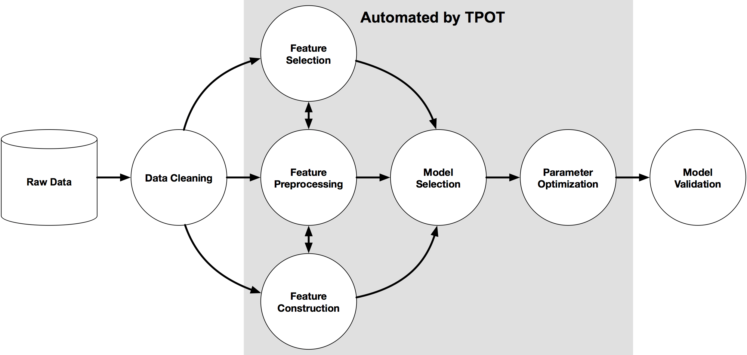
Another popular AutoML library is TPOT, which stands for Tree-Based Pipeline Optimization Tool. The goal of TPOT is to automate the building of ML pipelines by combining a flexible expression tree representation of pipelines with stochastic search algorithms such as genetic programming. TPOT makes use of the Python-based scikit-learn library
Install the TPOT library using
pip3 install tpotHere is an example tree-based pipeline from TPOT. Each circle corresponds to a machine learning operator, and the arrows indicate the direction of the data flow

Let’s build upon my previous blog post on AutomML, by using the same data set, with no modifications, and using the training (X_train, y_train) and test (X_test, y_test) data sets (dataframes), based on the Bank data sets. Check the previous post for the detailed steps on getting to this point.
In a similar way as the autosklean library example, I’m just going to demonstrate using TPOT for a classification problem using TPOTClassifier class. For regression problems, there is the corresponding TPOTRegressor class (not demonstrated in this post).
TPOTClassifier has the following main parameters (there are others):
- generations: Number of iterations to the run pipeline optimization process. The default is 100.
- population_size: Number of individuals to retain in the genetic programming population every generation. The default is 100.
- offspring_size: Number of offspring to produce in each genetic programming generation. The default is 100.
- mutation_rate: Mutation rate for the genetic programming algorithm in the range [0.0, 1.0]. This parameter tells the GP algorithm how many pipelines to apply random changes to every generation. Default is 0.9
- crossover_rate: Crossover rate for the genetic programming algorithm in the range [0.0, 1.0]. This parameter tells the genetic programming algorithm how many pipelines to “breed” every generation.
- scoring: Function used to evaluate the quality of a given pipeline for the classification problem like
accuracy,average_precision,roc_auc,recall, etc. The default isaccuracy. - cv: Cross-validation strategy used when evaluating pipelines. The default is 5.
- random_state: The seed of the pseudo-random number generator used in TPOT. Use this parameter to make sure that TPOT will give you the same results each time you run it against the same data set with that seed.
- verbosity: How much information TPOT communicates while it is running. Default is 0 (zero) TPOT will display nothing. 1=display minimal information, 2=display more information and progress bar, 3=print everything and progress bar.
- n_jobs: Number of processes to use. Default is 1. Use -1 to use all available cores.
Care is needed with some of these settings, for example generations should be set small to begin with, for example set to 5 initially. Also, population_size should also be kept small, for example 5 initially. These initial settings will evaluate 25 piplelines (5×5) configurations before finishing, and for some these settings may need to be adjusted smaller for initial work/investigations. Another parameter to adjust is the ‘verbosity’ setting. The default is 0 which means no details will be displayed. I like to set this to 3, as it gives more details of the outcomes from each pipeline. Adjust higher for more details or lower to fewer details. Another parameter to consider adjusting is ‘max_time_min’ and ‘max_eval_time_min’, but setting these too low can result in no or minimum results.
Load the library, setup the configuration and run. This is very simple to setup
from tpot import TPOTClassifier

#configure settings
tpot = TPOTClassifier(generations=5, population_size=5, verbosity=3, n_jobs=4, scoring='accuracy')

#run TPOT
tpot.fit(X_train, y_train)
As verbosity is set to 3 we get a lot of detail being displayed for each generation. The final output is shown below. What is missing from this is the progress bars which are displayed while TPOT is running
32 operators have been imported by TPOT.


Generation 1 - Current Pareto front scores:

-1	0.8963961891371728	RandomForestClassifier(input_matrix, RandomForestClassifier__bootstrap=True, RandomForestClassifier__criterion=gini, RandomForestClassifier__max_features=0.7000000000000001, RandomForestClassifier__min_samples_leaf=5, RandomForestClassifier__min_samples_split=7, RandomForestClassifier__n_estimators=100)

-2	0.8978183008194085	RandomForestClassifier(ZeroCount(input_matrix), RandomForestClassifier__bootstrap=True, RandomForestClassifier__criterion=gini, RandomForestClassifier__max_features=0.7000000000000001, RandomForestClassifier__min_samples_leaf=5, RandomForestClassifier__min_samples_split=7, RandomForestClassifier__n_estimators=100)
Pipeline encountered that has previously been evaluated during the optimization process. Using the score from the previous evaluation.

Generation 2 - Current Pareto front scores:

-1	0.8974020496851336	RandomForestClassifier(input_matrix, RandomForestClassifier__bootstrap=True, RandomForestClassifier__criterion=gini, RandomForestClassifier__max_features=0.7000000000000001, RandomForestClassifier__min_samples_leaf=8, RandomForestClassifier__min_samples_split=7, RandomForestClassifier__n_estimators=100)

-2	0.8978183008194085	RandomForestClassifier(ZeroCount(input_matrix), RandomForestClassifier__bootstrap=True, RandomForestClassifier__criterion=gini, RandomForestClassifier__max_features=0.7000000000000001, RandomForestClassifier__min_samples_leaf=5, RandomForestClassifier__min_samples_split=7, RandomForestClassifier__n_estimators=100)
_pre_test decorator: _random_mutation_operator: num_test=0 '(slice(None, None, None), 0)' is an invalid key.
Pipeline encountered that has previously been evaluated during the optimization process. Using the score from the previous evaluation.

Generation 3 - Current Pareto front scores:

-1	0.8974020496851336	RandomForestClassifier(input_matrix, RandomForestClassifier__bootstrap=True, RandomForestClassifier__criterion=gini, RandomForestClassifier__max_features=0.7000000000000001, RandomForestClassifier__min_samples_leaf=8, RandomForestClassifier__min_samples_split=7, RandomForestClassifier__n_estimators=100)

-2	0.8978183008194085	RandomForestClassifier(ZeroCount(input_matrix), RandomForestClassifier__bootstrap=True, RandomForestClassifier__criterion=gini, RandomForestClassifier__max_features=0.7000000000000001, RandomForestClassifier__min_samples_leaf=5, RandomForestClassifier__min_samples_split=7, RandomForestClassifier__n_estimators=100)
Skipped pipeline #21 due to time out. Continuing to the next pipeline.
Skipped pipeline #23 due to time out. Continuing to the next pipeline.

Generation 4 - Current Pareto front scores:

-1	0.8974020496851336	RandomForestClassifier(input_matrix, RandomForestClassifier__bootstrap=True, RandomForestClassifier__criterion=gini, RandomForestClassifier__max_features=0.7000000000000001, RandomForestClassifier__min_samples_leaf=8, RandomForestClassifier__min_samples_split=7, RandomForestClassifier__n_estimators=100)

-2	0.8978183008194085	RandomForestClassifier(ZeroCount(input_matrix), RandomForestClassifier__bootstrap=True, RandomForestClassifier__criterion=gini, RandomForestClassifier__max_features=0.7000000000000001, RandomForestClassifier__min_samples_leaf=5, RandomForestClassifier__min_samples_split=7, RandomForestClassifier__n_estimators=100)

Generation 5 - Current Pareto front scores:

-1	0.8983385200075953	RandomForestClassifier(input_matrix, RandomForestClassifier__bootstrap=True, RandomForestClassifier__criterion=gini, RandomForestClassifier__max_features=0.55, RandomForestClassifier__min_samples_leaf=8, RandomForestClassifier__min_samples_split=7, RandomForestClassifier__n_estimators=100)

TPOTClassifier(generations=5, n_jobs=4, population_size=5, scoring='accuracy',
               verbosity=3)
We can now display the ‘best’ model configuration discovered by TPOT.
tpot.fitted_pipeline_


Pipeline(steps=[('normalizer', Normalizer(norm='l1')),
                ('xgbclassifier',
                 XGBClassifier(base_score=0.5, booster='gbtree',
                               colsample_bylevel=1, colsample_bynode=1,
                               colsample_bytree=1, gamma=0, gpu_id=-1,
                               importance_type='gain',
                               interaction_constraints='', learning_rate=0.01,
                               max_delta_step=0, max_depth=8,
                               min_child_weight=7, missing=nan,
                               monotone_constraints='()', n_estimators=100,
                               n_jobs=1, num_parallel_tree=1, random_state=0,
                               reg_alpha=0, reg_lambda=1, scale_pos_weight=1,
                               subsample=0.8, tree_method='exact',
                               validate_parameters=1, verbosity=0))])
In this run of TPOT, on this data set, XGBoost algorithm gave the best results using the parameters and settings listed above. What is interesting, everytime I’ve run TPOT for the same data set, using the same configuration parameters, I get a slightly different outcome.
Next step is to evaluate the ‘best’ model on the holdout data set.
tpot.score(X_test, y_test)


0.9037792344420167
The results achieved are good and are better than some of the other models created by other AutoML libraries.
The final step we can perform is to export the model template. This creates a file containing the template code to create and use the model. This does require some modifications to specify the data set, and the pipeline of data modifications and transformations.
#export the model
tpot.export('.../tpot_Bank_pipeline.py')
The output file contains the following.
import numpy as np
import pandas as pd
from sklearn.model_selection import train_test_split
from sklearn.pipeline import make_pipeline
from sklearn.preprocessing import Normalizer
from xgboost import XGBClassifier

# NOTE: Make sure that the outcome column is labeled 'target' in the data file
tpot_data = pd.read_csv('PATH/TO/DATA/FILE', sep='COLUMN_SEPARATOR', dtype=np.float64)
features = tpot_data.drop('target', axis=1)

training_features, testing_features, training_target, testing_target = \
            train_test_split(features, tpot_data['target'], random_state=None)

# Average CV score on the training set was: 0.8986507248984001
exported_pipeline = make_pipeline(
    Normalizer(norm="l1"),
    XGBClassifier(learning_rate=0.01, max_depth=8, min_child_weight=7, n_estimators=100, n_jobs=1, subsample=0.8, verbosity=0)
)

exported_pipeline.fit(training_features, training_target)
results = exported_pipeline.predict(testing_features)
TPOT does have some issues and limitations. Well it is slow, and part of this is due to the nature of genetic algorithms, every time you run TPOT you may get different results, etc. Some of these issues can be addressed by adjusting some of the parameters, but even still, it doesn’t eliminate all of them. Running on GPU helps a little with timing of each run. TPOT doesn’t remove the need for data cleaning, feature engineering etc, but that is the case with most solutions.
AutoML – using autosklearn in Python
I’ve written some previous posts about AutoML and how to use AutoML with Oracle OML4Py (part 1 and part 2) and AutoML UI.
Building upon these, in this post I’ll demonstrate how to use autosklearn Python Package to do something similar, using the same data set I used in my previous posts.
To install the package run the typical pip command
pip3 install auto-sklearn
I did have some challegenges with installing this package, and this seems to be common, with different people having slightly different issues. These mainly revolved around having to install/update the swiff and pyrfr Python packages. Once done, then autosklearn package installed.
Let’s do a simple test
import autosklearn
print('autosklearn: %s' % autosklearn.__version__)

autosklearn: 0.12.5
Just like in my previous examples, I’m just going to use autosklearn to build a Classification model, as that is what the data set is designed for.
from sklearn.metrics import accuracy_score

# define search
model = autosklearn.classification.AutoSklearnClassifier()
# perform the search
model.fit(X_train, y_train)
The code above is a very basic configuration, and if this is the first time you are going to run this, then DON’T. There are a lot of parameter you can set, with one of them being ‘time_left_for_this_task’. The default value for this parameter is 360, which is one hour. Not a good idea! Set this to being much lower, say for an initial run of 3-5 minutes. This should be enough time for it to build many different models. I like to set the time for this using a multiplier of 60 (seconds). That way you don’t have to do any calculations! Two other parameters to consider setting/changing are
- n_jobs: this is the number of jobs to run in parallel. Default is -1, which uses all processors, or set to to a number, eg. 4
- metric: what evaluation metric to use for the models. For classification we have, accuracy, balanced_accuracy, f1, f1_marco, f1_micro, f1_samples, f1_weighted, roc_auc, precision, precision_macro, precision_micro, precision_samples, precision_weighted, average_percision, recall, recall_macro, recall_micro, recall_samples, recall_weighted and log_loss. For regression problems, r2, mean_squared_error, mean_absolute_error and median_absolute_error
Using these parameters let’s run a search.
# define search
model2 = autosklearn.classification.AutoSklearnClassifier(time_left_for_this_task=2*60,
      n_jobs=-1,
      metric=autosklearn.metrics.accuracy)

# perform the search
model2.fit(X_train, y_train)

Out[]: AutoSklearnClassifier(metric=accuracy, n_jobs=-1, per_run_time_limit=48,
                      time_left_for_this_task=120)
After about 2 minutes we explore the models.
print(model2.show_models())

[(0.520000, SimpleClassificationPipeline({'balancing:strategy': 'none', 'classifier:__choice__': 'random_forest', 'data_preprocessing:categorical_transformer:categorical_encoding:__choice__': 'one_hot_encoding', 'data_preprocessing:categorical_transformer:category_coalescence:__choice__': 'minority_coalescer', 'data_preprocessing:numerical_transformer:imputation:strategy': 'mean', 'data_preprocessing:numerical_transformer:rescaling:__choice__': 'standardize', 'feature_preprocessor:__choice__': 'no_preprocessing', 'classifier:random_forest:bootstrap': 'True', 'classifier:random_forest:criterion': 'gini', 'classifier:random_forest:max_depth': 'None', 'classifier:random_forest:max_features': 0.5, 'classifier:random_forest:max_leaf_nodes': 'None', 'classifier:random_forest:min_impurity_decrease': 0.0, 'classifier:random_forest:min_samples_leaf': 1, 'classifier:random_forest:min_samples_split': 2, 'classifier:random_forest:min_weight_fraction_leaf': 0.0, 'data_preprocessing:categorical_transformer:category_coalescence:minority_coalescer:minimum_fraction': 0.01},
dataset_properties={
  'task': 1,
  'sparse': False,
  'multilabel': False,
  'multiclass': False,
  'target_type': 'classification',
  'signed': False})),
(0.480000, SimpleClassificationPipeline({'balancing:strategy': 'none', 'classifier:__choice__': 'random_forest', 'data_preprocessing:categorical_transformer:categorical_encoding:__choice__': 'no_encoding', 'data_preprocessing:categorical_transformer:category_coalescence:__choice__': 'minority_coalescer', 'data_preprocessing:numerical_transformer:imputation:strategy': 'most_frequent', 'data_preprocessing:numerical_transformer:rescaling:__choice__': 'standardize', 'feature_preprocessor:__choice__': 'feature_agglomeration', 'classifier:random_forest:bootstrap': 'True', 'classifier:random_forest:criterion': 'entropy', 'classifier:random_forest:max_depth': 'None', 'classifier:random_forest:max_features': 0.48846965177813817, 'classifier:random_forest:max_leaf_nodes': 'None', 'classifier:random_forest:min_impurity_decrease': 0.0, 'classifier:random_forest:min_samples_leaf': 1, 'classifier:random_forest:min_samples_split': 5, 'classifier:random_forest:min_weight_fraction_leaf': 0.0, 'data_preprocessing:categorical_transformer:category_coalescence:minority_coalescer:minimum_fraction': 0.01087424610670389, 'feature_preprocessor:feature_agglomeration:affinity': 'cosine', 'feature_preprocessor:feature_agglomeration:linkage': 'complete', 'feature_preprocessor:feature_agglomeration:n_clusters': 17, 'feature_preprocessor:feature_agglomeration:pooling_func': 'median'},
dataset_properties={
  'task': 1,
  'sparse': False,
  'multilabel': False,
  'multiclass': False,
  'target_type': 'classification',
  'signed': False})),
]
In this particular case it has evaluated two models and we can display some basic statistics about this process.
# summarize
print(model2.sprint_statistics())

auto-sklearn results:
  Dataset name: ecd21bb4-912e-11eb-8af6-acde48001122
  Metric: accuracy
  Best validation score: 0.895218
  Number of target algorithm runs: 12
  Number of successful target algorithm runs: 2
  Number of crashed target algorithm runs: 0
  Number of target algorithms that exceeded the time limit: 10
  Number of target algorithms that exceeded the memory limit: 0
It only had time to create and evaluate 2 models, returning the best model. This can use this model to evaluate results from the holdout test data set.
# evaluate best model
y_predictions = model2.predict(X_test)
acc = accuracy_score(y_test, y_predictions)
print("Accuracy: %.3f" % acc)

Accuracy: 0.900
Now change the run time to see how many extra models will be evaluated in the time. The following increases the run time from 2 to 3 minutes. The evaluation metric has been changed to the f1 score.
# define search
model3 = autosklearn.classification.AutoSklearnClassifier(time_left_for_this_task=3*60,
      n_jobs=4,
      metric=autosklearn.metrics.f1) #accuracy)  #roc_auc   f1)
# perform the search
model3.fit(X_train, y_train)

AutoSklearnClassifier(metric=f1, n_jobs=4, per_run_time_limit=72,
                      time_left_for_this_task=180)
The statistics tells us it evaluated 7 models, out of a target of 15.
# summarize
print(model3.sprint_statistics())

auto-sklearn results:
  Dataset name: 752a4fc6-9135-11eb-8af6-acde48001122
  Metric: f1
  Best validation score: 0.473426
  Number of target algorithm runs: 15
  Number of successful target algorithm runs: 7
  Number of crashed target algorithm runs: 0
  Number of target algorithms that exceeded the time limit: 8
  Number of target algorithms that exceeded the memory limit: 0
The output from the ‘show_models’ function is too long to show here, but you should run it to see the details.
There is a package/library called PipelineProfiler, which is a VERY useful tool for inspecting the various models created and evaluated in the above process. It allows us to see, for each model run, what steps and algorithms were part of it, and by clicking on one we get a flow chart of the pipleline. An example is shown below.
import PipelineProfiler

profiler_data= PipelineProfiler.import_autosklearn(model3)
PipelineProfiler.plot_pipeline_matrix(profiler_data)
Listed in 2 categories of “Who’s Who in Data Science & Machine Learning?”
I’ve received notification I’ve been listed in the “Who’s Who in Data Science & Machine Learning?” lists created by Onalytica. I’ve been listed in not just one category but two categories. These are:
- Key Opinion Leaders discussing Data Science & Machine Learning
- Big Data
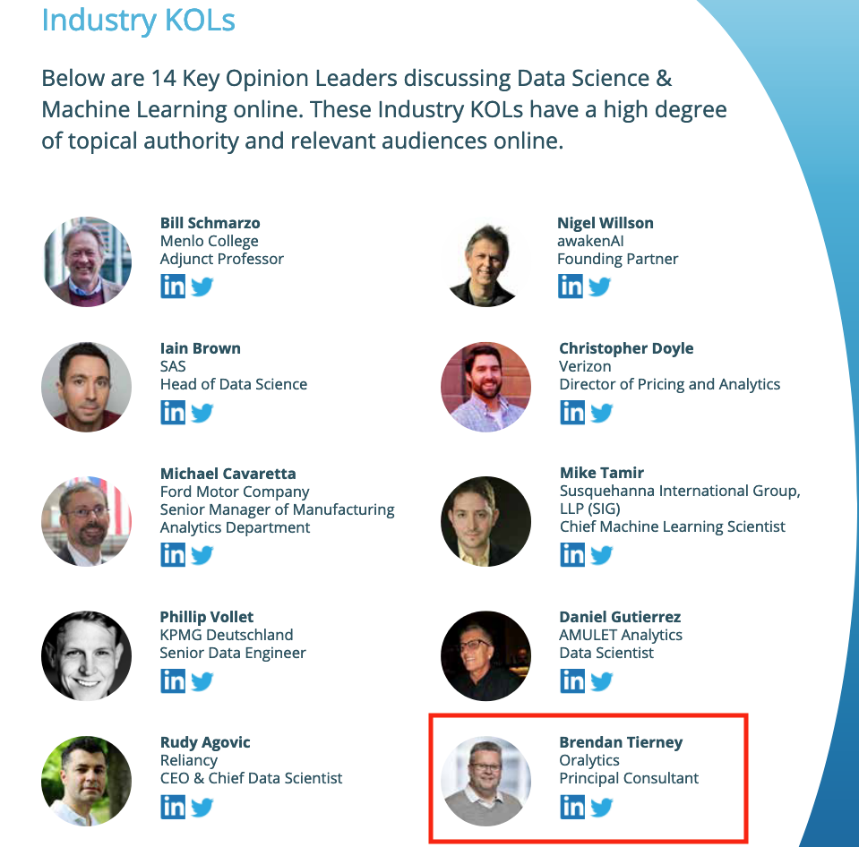
This is what Onalytica says about their report and how the list for each category was put together. “The influential experts are selected using Onalytica’s 4 Rs methodology (Reach, Resonance, Relevance and Reference). Quantitative data is pulled through LinkedIn, Twitter, Personal Blogs, YouTube, Podcast, and Forbes channels, and our qualitative data is pulled by our insights and analytics team, capturing offline influenc”. “All the influential experts featured are categorised by influencer persona, the sector they work in, their role within that sector, and more from our curated database of 1m+ influencers”. “Our Who’s Who lists are created using the Onalytica platform which has a curated database of over 1 million influencers. Our platform allows you to discover, validate and categorise influencers quickly and easily via keyword searches. Our lists are made using carefully created Boolean queries which then rank influencers by resonance, relevance, reach and reference, meaning influencers are not only ranked by themselves, but also by how much other influencers are referring to them. The lists are then validated, and filters are used to split the influencers up into the categories that are seen in the list.”
Check out the full report on “Who’s Who in Data Science & Machine Learning?“
AutoML, what is it good for? It Depends!
Automated Machine Learning (AutoML) seems to be everywhere and every Analytics product and SaaS offering seems to have some element of AutoML built into them. Part of the reason for this is because most of the market analysts, such as Gartner etc., have been rating Machine Learning (ML) products and services based on them having an AutoML feature.

Some of the benefits of AutoML is it will automatically generate a ML model for you without you having to worry about any of the technical details and the various statistical tests to measure if the model is useful. This kind of message has resulted is lots and lots of articles talking about the death of the Data Scientist, as they are no longer needed. We must remember ML is only one of the tools and skills of the data scientist.
This can all sound great. No need to hire these expensive data scientists, I can just use this AutoML software to create a ML model, for my data, and life will be good with all these wonderful predictions. Just think of the money I’ll be making and saving!
Where the fun comes into all of this is when someone issues legal proceedings based on what one of these AutoML models has predicted. The AutoML has made an incorrect prediction. The problem you now face, probably in court, is trying to justify the prediction by saying the machine/computer/algorithm made it, and you have no idea how or what it is doing to make the prediction. Good luck in a court explaining that to a judge and/or jury. Be prepared to hand over lots of money
What is missing is the human in the loop, and in most cases this will be the data scientist or machine learning engineer (or someone else with a really cool job title). Part of their job is to evaluate lots of difference models for you data (remember they will create lots and lots of models and not just one!), determine (from experimentation) what algorithms work best with your data and problem, optimize these models and assess the impact of changing hyperparameters, look at how these ML models are behaving, are there any biases in the model or data, use a wide variety of statistic tests to assess the models, examine how the model works with different sub-parts of the data (customers), look at any potential legal and legislative issues not just in one geographic but across many disparate regions all of which have different legal requirements, etc.
As you can see there are many additional tasks beyond the ML steps needed to create, verify and select a ML to use. All of this is before you look at how it can be deployed in your production systems/architecture and building out you MLOps.
One importing characteristic of having the human in the loop is Explainability. Explainability of the process followed, what models were produced, the effect of tuning and opimizing, possible biases and mitigating steps, etc etc The list goes on and on. This the role of the data scientist and now it might look like a good idea to hire a good data scientist who understands all of this.

Taking a little step back, AutoML is kind of good cool feature/tool. A lot of the main steps of creating all those ML models, tuning them and evaluating them, etc can be very boring work. You do same steps for each model and do it all over again for the next, and so on for the tens or hundreds of models you will be creating. Most data scientists will have scripts in their toolbox (based from their experience) to automatically perform all of these steps and output the results. I mentioned the word experience in the last sentence. It can take a bit of time to build up to this. The AutoML products will do all of this automatically for you hence you don’t have to hire a data scientist to do it (see what I said above about this).
I mentioned above some of the challenges and the need to keep a human in the loop. AutoML can be seen as another tool to assist the data scientist and not to replace them. AutoML can be used to to help the data scientist work towards identifying what ML models to use. But this can be a bit of a challenge to do. It depends on what product or library you use. Some AutoML solutions act as a black box. Kind of like the image at the top of this post. These are simple to use but the draw back is there is not explainability or ability of the data scientist to really assess what is happening at each step. There are AutoML products/solutions that allow you to inspect and monitor what is happening at each step within AutoML. The diagram given able is one example of this. This allows for the human in the loop and allows for explainability. If the data scientist sees some unusual direction being taken by AutoML they can see where and why this is happening and can take corrective action. AutoML isn’t a black box in this scenario.
I mentioned above, AutoML can be another tool for the data scientist to use. Look on AutoML as quick way to see what might be possible. Using the information from each step of AutoML, the data scientist can use this information to guide them towards creating a more suitable and usable ML model, and do so in perhaps a slightly shorter space of time.
Going back to the title of the post ‘AutoML, what is it good for?’, the answer really is ‘It Depends!’, but if you do use it, be careful how you use the models and results beyond doing some simple investigation. And be careful of product offerings saying you don’t need anything else.

You must be logged in to post a comment.