
Big Data
Exploring Apache Iceberg – Part 3 – Parquet Files with Oracle Database
In this post I’ll explore how you can included data in Parquet files in an Oracle Database. This is a little sideways post from my previous posts on Apache Iceberg, as it will only look at using Parquet files, which are a core part of Iceberg tables, but is missing the meta-data layer that Iceberg tables gives.
The previous two posts on Apache Iceberg looked at using PyIceberg Python package to create and to explore the various feature of Iceberg and it’s effects on the data, files and meta-data. Part-1, Part-2.
We can include Parquet files in an Oracle Database by creating an External Table based on those files. Let’s walk through an example. The following example will for an “On-Premises” Database. I’ll have an example later in this post if you are using an Oracle Autonomous Database on Oracle Cloud.
Log into the Database as SYSTEM user, create a directory option to point to the location of the files on the operating system, and then grant privileges to the schama that needs to read that data.
CREATE OR REPLACE DIRECTORY parquet_dir AS '/data/log/parquet';GRANT READ, WRITE ON DIRECTORY parquet_dir TO parquet_user;
It is assumed the directory ‘/data/log/parquet‘ exists and has some parquet files in it.
Connect the schama “parquet_user” and create an External Table that points to the parquet files in the directory
CREATE TABLE parquet_sales_data ( sale_id NUMBER, sale_date DATE, product_id NUMBER, amount NUMBER(10,2), region VARCHAR2(50))ORGANIZATION EXTERNAL ( TYPE ORACLE_BIGDATA DEFAULT DIRECTORY parquet_dir ACCESS PARAMETERS ( com.oracle.bigdata.fileformat = PARQUET ) LOCATION ('sales_*.parquet'))REJECT LIMIT UNLIMITED;
We can not query the parquey data just like any other data in a table.
SELECT region, product, SUM(amount) AS total_salesFROM sales_externalGROUP BY regionORDER BY total_sales DESC;
Care is needed to ensure column name and datatypes match between the table and the parquet file.
If our parquet files are partitioned into directories for different time periods, we can create a Partitioned External Table to handle that data, and we it we get the benefits of partition pruning, etc and better response times.
CREATE TABLE parquet_sales_data ( sale_id NUMBER, sale_date DATE, product_id NUMBER, amount NUMBER(10,2), region VARCHAR2(50))ORGANIZATION EXTERNAL PARALLEL 4 ( TYPE ORACLE_BIGDATA DEFAULT DIRECTORY parquet_dir ACCESS PARAMETERS ( com.oracle.bigdata.fileformat = PARQUET )PARTITION BY LIST (region) ( PARTITION p_emea VALUES ('EMEA') LOCATION (emea_dir:'*.parquet'), PARTITION p_apac VALUES ('APAC') LOCATION (apac_dir:''*.parquet'), PARTITION p_amer VALUES ('AMER') LOCATION (amer_dir:'*.parquet'))REJECT LIMIT UNLIMITED;
For this example, I needed to connect as SYSTEM and create the extra directories to point to the additional directories used. I also added PARALLEL 4 to the table to help speed things up a little more.
Exploring Apache Iceberg using PyIceberg – Part 2
Apache Iceberg, an open-source table format that has become the industry standard for data sharing in modern data architectures. In my previous posts on Apache Iceberg I explored the core features of Iceberg Tables and gave examples of using Python code to create, store, add data, read a table and apply filters to an Iceberg Table. In this post I’ll explore some of the more advanced features of interacting with an Iceberg Table, how to add partitioning and how to moved data to a DuckDB database.
Check out the link at the bottom of this post to download the Notebook containing all the PyIceberg code in this post. I had a similar notebook for all the code examples in my previous post. You should check that our first as the examples in the post and notebook are an extension of those.
This post will cover:
- Partitioning an Iceberg Table
- Schema Evolution
- Row Level Operations
- Advanced Scanning & Query Patterns
- DuckDB and Iceberg Tables
Setup & Conguaration
Before we can start on the core aspects of this post, we need to do some basic setup like importing the necessary Python packages, defining the location of the warehouse and catalog and checking the namespace exists. These were created created in the previous post.
import os, pandas as pd, pyarrow as pafrom datetime import datefrom pyiceberg.catalog.sql import SqlCatalogfrom pyiceberg.schema import Schemafrom pyiceberg.types import ( NestedField, LongType, StringType, DoubleType, DateType)from pyiceberg.partitioning import PartitionSpec, PartitionFieldfrom pyiceberg.transforms import ( MonthTransform, IdentityTransform, BucketTransform)WAREHOUSE = "/Users/brendan.tierney/Dropbox/Iceberg-Demo"os.makedirs(WAREHOUSE, exist_ok=True)catalog = SqlCatalog("local", **{ "uri": f"sqlite:///{WAREHOUSE}/catalog.db", "warehouse": f"file://{WAREHOUSE}",})for ns in ["sales_db"]: if ns not in [n[0] for n in catalog.list_namespaces()]: catalog.create_namespace(ns)
Partitioning an Iceberg Table
Partitioning is how Iceberg physically organises data files on disk to enable partition pruning. Partitioning pruning will automactically skip directorys and files that don’t contain the data you are searching for. This can have a significant improvement of query response times.
The following will create a partition table based on the combination of the fiels order_date and region.
# ── Explicit Iceberg schema (gives us full control over field IDs) ─────schema = Schema( NestedField(field_id=1, name="order_id", field_type=LongType(), required=False), NestedField(field_id=2, name="customer", field_type=StringType(), required=False), NestedField(field_id=3, name="product", field_type=StringType(), required=False), NestedField(field_id=4, name="region", field_type=StringType(), required=False), NestedField(field_id=5, name="order_date", field_type=DateType(), required=False), NestedField(field_id=6, name="revenue", field_type=DoubleType(), required=False),)# ── Partition spec: partition by month(order_date) AND identity(region) ─partition_spec = PartitionSpec( PartitionField( source_id=5, # order_date field_id field_id=1000, transform=MonthTransform(), name="order_date_month", ), PartitionField( source_id=4, # region field_id field_id=1001, transform=IdentityTransform(), name="region", ),)tname = ("sales_db", "orders_partitioned")if catalog.table_exists(tname): catalog.drop_table(tname)
Now we can create the table and inspect the details
table = catalog.create_table( tname, schema=schema, partition_spec=partition_spec,)print("Partition spec:", table.spec())Partition spec: [ 1000: order_date_month: month(5) 1001: region: identity(4)]
We can now add data to the partitioned table.
# Write data — Iceberg routes each row to the correct partition directorydf = pd.DataFrame({ "order_id": [1001, 1002, 1003, 1004, 1005, 1006], "customer": ["Alice", "Bob", "Carol", "Dave", "Eve", "Frank"], "product": ["Laptop", "Phone", "Tablet", "Monitor", "Keyboard", "Webcam"], "region": ["EU", "US", "EU", "APAC", "US", "EU"], "order_date": [date(2024,1,15), date(2024,1,20), date(2024,2,3), date(2024,2,20), date(2024,3,5), date(2024,3,12)], "revenue": [1299.99, 1798.00, 549.50, 1197.00, 399.95, 258.00],})table.append(pa.Table.from_pandas(df))
We can inspect the directories and files created. I’ve only include a partical listing below but it should be enough for you to get and idea of what Iceberg as done.
# Verify partition directories were created!find {WAREHOUSE}/sales_db/orders_partitioned/data -type f/Users/brendan.tierney/Dropbox/Iceberg-Demo/sales_db/orders_partitioned/data/region=APAC/order_date_day=2024-04-05/00000-4-0542db6c-f67f-4a26-9012-59d8267b5005.parquet/Users/brendan.tierney/Dropbox/Iceberg-Demo/sales_db/orders_partitioned/data/region=APAC/order_date_day=2024-02-20/00000-2-0542db6c-f67f-4a26-9012-59d8267b5005.parquet/Users/brendan.tierney/Dropbox/Iceberg-Demo/sales_db/orders_partitioned/data/order_date_month=2024-01/region=EU/00000-0-e9ad65a0-c088-46fc-a537-12a6b60b38c5.parquet/Users/brendan.tierney/Dropbox/Iceberg-Demo/sales_db/orders_partitioned/data/order_date_month=2024-01/region=EU/00000-0-1f976101-f836-4db3-bf4a-c0e0cf7dd4c6.parquet/Users/brendan.tierney/Dropbox/Iceberg-Demo/sales_db/orders_partitioned/data/order_date_month=2024-01/region=EU/00000-0-4233dad6-ef48-4ad5-95c9-5842e641fc0f.parquet/Users/brendan.tierney/Dropbox/Iceberg-Demo/sales_db/orders_partitioned/data/order_date_month=2024-01/region=EU/00000-0-b0a10298-d2a6-45b4-a541-9a459e478496.parquet/Users/brendan.tierney/Dropbox/Iceberg-Demo/sales_db/orders_partitioned/data/order_date_month=2024-01/region=US/00000-1-b0a10298-d2a6-45b4-a541-9a459e478496.parquet/Users/brendan.tierney/Dropbox/Iceberg-Demo/sales_db/orders_partitioned/data/order_date_month=2024-01/region=US/00000-1-4233dad6-ef48-4ad5-95c9-5842e641fc0f.parquet/Users/brendan.tierney/Dropbox/Iceberg-Demo/sales_db/orders_partitioned/data/order_date_month=2024-01/region=US/00000-1-1f976101-f836-4db3-bf4a-c0e0cf7dd4c6.parquet/Users/brendan.tierney/Dropbox/Iceberg-Demo/sales_db/orders_partitioned/data/order_date_month=2024-01/region=US/00000-1-e9ad65a0-c088-46fc-a537-12a6b60b38c5.parquet/Users/brendan.tierney/Dropbox/Iceberg-Demo/sales_db/orders_partitioned/data/region=EU/order_date_day=2024-02-03/00000-1-0542db6c-f67f-4a26-9012-59d8267b5005.parquet/Users/brendan.tierney/Dropbox/Iceberg-Demo/sales_db/orders_partitioned/data/region=EU/order_date_day=2024-01-15/00000-0-0542db6c-f67f-4a26-9012-59d8267b5005.parquet/Users/brendan.tierney/Dropbox/Iceberg-Demo/sales_db/orders_partitioned/data/region=EU/order_date_day=2024-04-01/00000-3-0542db6c-f67f-4a26-9012-59d8267b5005.parquet/Users/brendan.tierney/Dropbox/Iceberg-Demo/sales_db/orders_partitioned/data/order_date_month=2024-02/region=APAC/00000-3-b0a10298-d2a6-45b4-a541-9a459e478496.parquet/Users/brendan.tierney/Dropbox/Iceberg-Demo/sales_db/orders_partitioned/data/order_date_month=2024-02/region=APAC/00000-3-e9ad65a0-c088-46fc-a537-12a6b60b38c5.parquet/Users/brendan.tierney/Dropbox/Iceberg-Demo/sales_db/orders_partitioned/data/order_date_month=2024-02/region=APAC/00000-3-4233dad6-ef48-4ad5-95c9-5842e641fc0f.parquet/Users/brendan.tierney/Dropbox/Iceberg-Demo/sales_db/orders_partitioned/data/order_date_month=2024-02/region=APAC/00000-3-1f976101-f836-4db3-bf4a-c0e0cf7dd4c6.parquet
We can change the partictioning specification without rearranging or reorganising the data
from pyiceberg.transforms import DayTransform# Iceberg can change the partition spec without rewriting old data.# Old files keep their original partitioning; new files use the new spec.with table.update_spec() as update: # Upgrade month → day granularity for more recent data update.remove_field("order_date_month") update.add_field( source_column_name="order_date", transform=DayTransform(), partition_field_name="order_date_day", )print("Updated spec:", table.spec())
I’ll leave you to explore the additional directories, files and meta-data files.
#find all files starting from this directory!find {WAREHOUSE}/sales_db/orders_partitioned/data -type f
Schema Evolution
Iceberg tracks every schema version with a numeric ID and never silently breaks existing readers. You can add, rename, and drop columns, change types (safely), and reorder fields, all with zero data rewriting.
#Add new columnsfrom pyiceberg.types import FloatType, BooleanType, TimestampTypeprint("Before:", table.schema())with table.update_schema() as upd: # Add optional columns — old files return NULL for these upd.add_column("discount_pct", FloatType(), "Discount percentage applied") upd.add_column("is_returned", BooleanType(), "True if the order was returned") upd.add_column("updated_at", TimestampType())print("After:", table.schema())Before: table { 1: order_id: optional long 2: customer: optional string 3: product: optional string 4: region: optional string 5: order_date: optional date 6: revenue: optional double}After: table { 1: order_id: optional long 2: customer: optional string 3: product: optional string 4: region: optional string 5: order_date: optional date 6: revenue: optional double 7: discount_pct: optional float (Discount percentage applied) 8: is_returned: optional boolean (True if the order was returned) 9: updated_at: optional timestamp}
We can rename columns. A column rename is a meta-data only change. The Parquet files are untouched. Older readers will still see the previous versions of the column name, whicl new readers will see the new column name.
#rename a columnwith table.update_schema() as upd: upd.rename_column("discount_pct", "discount_percent")print("Updated:", table.schema())Updated: table { 1: order_id: optional long 2: customer: optional string 3: product: optional string 4: region: optional string 5: order_date: optional date 6: revenue: optional double 7: discount_percent: optional float (Discount percentage applied) 8: is_returned: optional boolean (True if the order was returned) 9: updated_at: optional timestamp}
Similarly when dropping a column, it is a meta-data change
#drop a columnwith table.update_schema() as upd: upd.delete_column("updated_at")print("Updated:", table.schema())Updated: table { 1: order_id: optional long 2: customer: optional string 3: product: optional string 4: region: optional string 5: order_date: optional date 6: revenue: optional double 7: discount_percent: optional float (Discount percentage applied) 8: is_returned: optional boolean (True if the order was returned)}
We can see all the different changes or versions of the Iceberg Table schema.
import json, globmeta_files = sorted(glob.glob( f"{WAREHOUSE}/sales_db/orders_partitioned/metadata/*.metadata.json"))with open(meta_files[-1]) as f: meta = json.load(f)print(f"Total schema versions: {len(meta['schemas'])}")for s in meta["schemas"]: print(f" schema-id={s['schema-id']} fields={[f['name'] for f in s['fields']]}")Total schema versions: 4 schema-id=0 fields=['order_id', 'customer', 'product', 'region', 'order_date', 'revenue'] schema-id=1 fields=['order_id', 'customer', 'product', 'region', 'order_date', 'revenue', 'discount_pct', 'is_returned', 'updated_at'] schema-id=2 fields=['order_id', 'customer', 'product', 'region', 'order_date', 'revenue', 'discount_percent', 'is_returned', 'updated_at'] schema-id=3 fields=['order_id', 'customer', 'product', 'region', 'order_date', 'revenue', 'discount_percent', 'is_returned']
Agian if you inspect the directories and files in the warehouse, you’ll see the impact of these changes at the file system level.
#find all files starting from this directory!find {WAREHOUSE}/sales_db/orders_partitioned/data -type f
Row Level Operations
Iceberg v2 introduces two delete file formats that enable row-level mutations without rewriting entire data files immediately — writes stay fast, and reads merge deletes on the fly.
Operations Iceberg Mechanism Write cost Read cost Append New data files only Low Low Delete rows Position or equality delete files Low Medium Update rows Delete + new data file Medium Medium (copy-on-write or merge-on-read) Overwrite Atomic swap of data files Medium Low (replace partition).
from pyiceberg.expressions import EqualTo, In# Delete all orders from the APAC regiontable.delete(EqualTo("region", "APAC"))print(table.scan().to_pandas()) order_id customer product region order_date revenue discount_percent \0 1001 Alice Laptop EU 2024-01-15 1299.99 NaN 1 1002 Bob Phone US 2024-01-20 1798.00 NaN 2 1003 Carol Tablet EU 2024-02-03 549.50 NaN 3 1005 Eve Keyboard US 2024-03-05 399.95 NaN 4 1006 Frank Webcam EU 2024-03-12 258.00 NaN is_returned 0 None 1 None 2 None 3 None 4 None
Also
# Delete specific order IDstable.delete(In("order_id", [1001, 1003]))# Verify — deleted rows are gone from the logical viewdf_after = table.scan().to_pandas()print(f"Rows after delete: {len(df_after)}")print(df_after[["order_id", "customer", "region"]])Rows after delete: 3 order_id customer region0 1002 Bob US1 1005 Eve US2 1006 Frank EU
We can see partiton pruning in action with a scan EqualTo(“region”, “EU”) will skip all data files in region=US/ and region=APAC/ directories entirely — zero bytes read from those files.
Advanced Scanning & Query Processing
The full expression API (And, Or, Not, In, NotIn, StartsWith, IsNull), time travel by snapshot ID, incremental reads between two snapshots for CDC pipelines, and streaming via Arrow RecordBatchReader for out-of-memory processing.
PyIceberg’s scan API supports rich predicate pushdown, snapshot-based time travel, incremental reads between snapshots, and streaming via Arrow record batches.
Let’s start by adding some data back into the table.
df3 = pd.DataFrame({ "order_id": [1001, 1003, 1004, 1006, 1007], "customer": ["Alice", "Carol", "Dave", "Frank", "Grace"], "product": ["Laptop", "Tablet", "Monitor", "Headphones", "Webcam"], "order_date": [ date(2024, 1, 15), date(2024, 2, 3), date(2024, 2, 20), date(2024, 4, 1), date(2024, 4, 5)], "region": ["EU", "EU", "APAC", "EU", "APAC"], "revenue": [1299.99, 549.50, 1197, 498.00, 129.00]})#Add the datatable.append(pa.Table.from_pandas(df3))
Let’s try a query with several predicates.
from pyiceberg.expressions import ( And, Or, Not, EqualTo, NotEqualTo, GreaterThan, GreaterThanOrEqual, LessThan, LessThanOrEqual, In, NotIn, IsNull, IsNaN, StartsWith,)# EU or US orders, revenue > 500, product is not "Keyboard"df_complex = table.scan( row_filter=And( Or( EqualTo("region", "EU"), EqualTo("region", "US"), ), GreaterThan("revenue", 500.0), NotEqualTo("product", "Keyboard"), ), selected_fields=("order_id", "customer", "product", "region", "revenue"),).to_pandas()print(df_complex) order_id customer product region revenue0 1001 Alice Laptop EU 1299.991 1003 Carol Tablet EU 549.502 1002 Bob Phone US 1798.00
Now let’s try a NOT predicate
df_not_in = table.scan( row_filter=Not(In("region", ["US", "APAC"]))).to_pandas()print(df_not_in) order_id customer product region order_date revenue \0 1001 Alice Laptop EU 2024-01-15 1299.99 1 1003 Carol Tablet EU 2024-02-03 549.50 2 1006 Frank Headphones EU 2024-04-01 498.00 3 1006 Frank Webcam EU 2024-03-12 258.00 discount_percent is_returned 0 NaN None 1 NaN None 2 NaN None 3 NaN None
Now filter data with data starting with certain values.
df_starts = table.scan( row_filter=StartsWith("product", "Lap") # matches "Laptop", "Laptop Pro").to_pandas()print(df_starts) order_id customer product region order_date revenue discount_percent \0 1001 Alice Laptop EU 2024-01-15 1299.99 NaN is_returned 0 None
Using the LIMIT function.
df_sample = table.scan(limit=3).to_pandas()print(df_sample) order_id customer product region order_date revenue discount_percent \0 1001 Alice Laptop EU 2024-01-15 1299.99 NaN 1 1003 Carol Tablet EU 2024-02-03 549.50 NaN 2 1004 Dave Monitor APAC 2024-02-20 1197.00 NaN is_returned 0 None 1 None 2 None
We can also perform data streaming.
# Process very large tables without loading everything into memory at oncescan = table.scan(selected_fields=("order_id", "revenue"))total_revenue = 0.0total_rows = 0# to_arrow_batch_reader() returns an Arrow RecordBatchReaderfor batch in scan.to_arrow_batch_reader(): df_chunk = batch.to_pandas() total_revenue += df_chunk["revenue"].sum() total_rows += len(df_chunk)print(f"Total rows: {total_rows}")print(f"Total revenue: ${total_revenue:,.2f}")Total rows: 8Total revenue: $6,129.44
DuckDB and Iceberg Tables
We can register an Iceberg scan plan as a DuckDB virtual table. PyIceberg handles metadata; DuckDB reads the Parquet files.
conn = duckdb.connect()# Expose the scan plan as an Arrow dataset DuckDB can queryscan = table.scan()arrow_dataset = scan.to_arrow() # or to_arrow_batch_reader()conn.register("orders", arrow_dataset)# Full SQL on the tableresult = conn.execute(""" SELECT region, COUNT(*) AS order_count, ROUND(SUM(revenue), 2) AS total_revenue, ROUND(AVG(revenue), 2) AS avg_revenue, ROUND(MAX(revenue) - MIN(revenue), 2) AS revenue_range FROM orders GROUP BY region ORDER BY total_revenue DESC""").df()print(result) region order_count total_revenue avg_revenue revenue_range0 EU 4 2605.49 651.37 1041.991 US 2 2197.95 1098.97 1398.052 APAC 2 1326.00 663.00 1068.00
DuckDB has a native Iceberg extension that reads Parquet files directly.
import duckdb, globconn = duckdb.connect()conn.execute("INSTALL iceberg; LOAD iceberg;")# Enable version guessing for Iceberg tablesconn.execute("SET unsafe_enable_version_guessing = true;")# Point DuckDB at the Iceberg table root directorytable_path = f"{WAREHOUSE}/sales_db/orders_partitioned"df_duck = conn.execute(f""" SELECT * FROM iceberg_scan('{table_path}', allow_moved_paths = true) WHERE revenue > 500 ORDER BY revenue DESC""").df()print(df_duck) order_id customer product region order_date revenue discount_percent \0 1002 Bob Phone US 2024-01-20 1798.00 NaN 1 1001 Alice Laptop EU 2024-01-15 1299.99 NaN 2 1004 Dave Monitor APAC 2024-02-20 1197.00 NaN 3 1003 Carol Tablet EU 2024-02-03 549.50 NaN is_returned 0 <NA> 1 <NA> 2 <NA> 3 <NA>
We can access the data using the time travel Iceberg feature.
# Time travel via DuckDBsnap_id = table.history()[0].snapshot_iddf_tt = conn.execute(f""" SELECT * FROM iceberg_scan( '{table_path}', snapshot_from_id = {snap_id}, allow_moved_paths = true )""").df()print(f"Time travel rows: {len(df_tt)}")Time travel rows: 6
Exploring Apache Iceberg using PyIceberg – Part 1
Apache Iceberg, an open-source table format that has become the industry standard for data sharing in modern data architectures. In a previous post I explored the core feature of Apache Iceberg and compared it with related technologies such as Apache Hudi and Delta Lake.
In this post we’ll look at some of the inital steps to setup and explore Iceberg tables using Python. I’ll have follow-on posts which will explore more advanced features of Apache Iceberg, again using Python. In this post, we’ll explore the following:
- Environmental setup
- Create an Iceberg Table from a Pandas dataframae
- Explore the Iceberg Table and file system
- Appending data and Time Travel
- Read an Iceberg Table into a Pandas dataframe
- Filtered scans with push-down predicates
Check out the link at the bottom of this post to download the Notebook containing all the PyIceberg code.
Environmental setup
Before we can get started with Apache Iceberg, we need to install it in our environment. I’m going with using Python for these blog posts and that means we need to install PyIceberg. In addition to this package, we also need to install pyiceberg-core. This is needed for some additional feature and optimisations of Iceberg.
pip install "pyiceberg[pyiceberg-core]"
This is a very quick install.
Next we need to do some environmental setup, like importing various packages used in the example code, setuping up some directories on the OS where the Iceberg files will be stored, creating a Catalog and a Namespace.
# Import other packages for this Demo Notebookimport pyarrow as paimport pandas as pdfrom datetime import dateimport osfrom pyiceberg.catalog.sql import SqlCatalog#define location for the WAREHOUSE, where the Iceberg files will be locatedWAREHOUSE = "/Users/brendan.tierney/Dropbox/Iceberg-Demo"#create the directory, True = if already exists, then don't report an erroros.makedirs(WAREHOUSE, exist_ok=True)#create a local Catalogcatalog = SqlCatalog( "local", **{ "uri": f"sqlite:///{WAREHOUSE}/catalog.db", "warehouse": f"file://{WAREHOUSE}", })#create a namespace (a bit like a database schema)NAMESPACE = "sales_db"if NAMESPACE not in [ns[0] for ns in catalog.list_namespaces()]: catalog.create_namespace(NAMESPACE)
That’s the initial setup complete.
Create an Iceberg Table from a Pandas dataframe
We can not start creating tables in Iceberg. To do this, the following code examples will initially create a Pandas dataframe, will convert it from table to columnar format (as the data will be stored in Parquet format in the Iceberg table), and then create and populate the Iceberg table.
#create a Pandas DF with some basic data# Create a sample sales DataFramedf = pd.DataFrame({ "order_id": [1001, 1002, 1003, 1004, 1005], "customer": ["Alice", "Bob", "Carol", "Dave", "Eve"], "product": ["Laptop", "Phone", "Tablet", "Monitor", "Keyboard"], "quantity": [1, 2, 1, 3, 5], "unit_price": [1299.99, 899.00, 549.50, 399.00, 79.99], "order_date": [ date(2024, 1, 15), date(2024, 1, 16), date(2024, 2, 3), date(2024, 2, 20), date(2024, 3, 5)], "region": ["EU", "US", "EU", "APAC", "US"]})# Compute total revenue per orderdf["revenue"] = df["quantity"] * df["unit_price"]print(df)print(df.dtypes) order_id customer product quantity unit_price order_date region \0 1001 Alice Laptop 1 1299.99 2024-01-15 EU 1 1002 Bob Phone 2 899.00 2024-01-16 US 2 1003 Carol Tablet 1 549.50 2024-02-03 EU 3 1004 Dave Monitor 3 399.00 2024-02-20 APAC 4 1005 Eve Keyboard 5 79.99 2024-03-05 US revenue 0 1299.99 1 1798.00 2 549.50 3 1197.00 4 399.95 order_id int64customer objectproduct objectquantity int64unit_price float64order_date objectregion objectrevenue float64dtype: object
That’s the Pandas dataframe created. Now we can convert it to columnar format using PyArrow.
#Convert pandas DataFrame → PyArrow Table # PyIceberg writes via Arrow (columnar format), so this step is requiredarrow_table = pa.Table.from_pandas(df)print("Arrow schema:")print(arrow_table.schema)Arrow schema:order_id: int64customer: stringproduct: stringquantity: int64unit_price: doubleorder_date: date32[day]region: stringrevenue: double-- schema metadata --pandas: '{"index_columns": [{"kind": "range", "name": null, "start": 0, "' + 1180
Now we can define the Iceberg table along with the namespace for it.
#Create an Iceberg table from the Arrow schemaTABLE_NAME = (NAMESPACE, "orders")table = catalog.create_table( TABLE_NAME, schema=arrow_table.schema,)tableorders( 1: order_id: optional long, 2: customer: optional string, 3: product: optional string, 4: quantity: optional long, 5: unit_price: optional double, 6: order_date: optional date, 7: region: optional string, 8: revenue: optional double),partition by: [],sort order: [],snapshot: null
The table has been defined in Iceberg and we can see there are no partitions, snapshots, etc. The Iceberg table doesn’t have any data. We can Append the Arrow table data to the Iceberg table.
#add the data to the tabletable.append(arrow_table)#table.append() adds new data files without overwriting existing ones. #Use table.overwrite() to replace all data in a single atomic operation.
We can look at the file system to see what has beeb written.
print(f"Table written to: {WAREHOUSE}/sales_db/orders/")print(f"Snapshot ID: {table.current_snapshot().snapshot_id}")Table written to: /Users/brendan.tierney/Dropbox/Iceberg-Demo/sales_db/orders/Snapshot ID: 3939796261890602539
Explore the Iceberg Table and File System
And Iceberg Table is just a collection of files on the file system, organised into a set of folders. You can look at these using your file system app, or use a terminal window, or in the examples below are from exploring those directories and files from a Jupyter Notebook.
Let’s start at the Warehouse level. This is the topic level that was declared back when the Environment was being setup. Check that out above in the first section.
!ls -l {WAREHOUSE}-rw-r--r--@ 1 brendan.tierney staff 20480 28 Feb 15:26 catalog.dbdrwxr-xr-x@ 3 brendan.tierney staff 96 28 Feb 12:59 sales_db
We can see the catalog file and a directiory for our ‘sales_db’ namespace. When you explore the contents of this file you will find two directorys. These contain the ‘metadata’ and the ‘data’ files. The following list the files found in the ‘data’ directory containing the data and these are stored in parquet format.
!ls -l {WAREHOUSE}/sales_db/orders/data-rw-r--r--@ 1 brendan.tierney staff 3179 28 Feb 15:22 00000-0-357c029e-b420-459b-8248-b1caf3c030ce.parquet-rw-r--r--@ 1 brendan.tierney staff 3307 28 Feb 15:23 00000-0-3fae55d7-1229-448c-9ffb-ae33c77003a3.parquet-rw-r--r--@ 1 brendan.tierney staff 3179 28 Feb 15:03 00000-0-4ec1ef74-cd24-412e-a35f-bcf3d745bf42.parquet-rw-r--r--@ 1 brendan.tierney staff 3179 28 Feb 15:23 00000-0-984ed6d2-4067-43c4-8c11-5f5a96febd24.parquet-rw-r--r-- 1 brendan.tierney staff 3307 28 Feb 15:26 00000-0-a61264e8-b361-490e-90f7-105a33f20dec.parquet-rw-r--r--@ 1 brendan.tierney staff 3307 28 Feb 15:22 00000-0-ac913dfe-548c-4cb3-99aa-4f1332e02248.parquet-rw-r--r--@ 1 brendan.tierney staff 3307 28 Feb 13:00 00000-0-b3fa23ec-79c6-48da-ba81-ba35f25aa7ad.parquet-rw-r--r--@ 1 brendan.tierney staff 3179 28 Feb 15:25 00000-0-d534a298-adab-4744-baa1-198395cc93bd.parquet-rw-r--r--@ 1 brendan.tierney staff 3307 28 Feb 15:21 00000-0-ef5dd6d8-84c0-4860-828e-86e4e175a9eb.parquet-rw-r--r--@ 1 brendan.tierney staff 3179 28 Feb 15:21 00000-0-f108db1c-39f9-4e2b-b825-3e580cccc808.parquet
I’ll leave you to explore the ‘metadata’ directory.
Read the Iceberg Table back into our Environment
To load an Iceberg table into your environment, you’ll need to load the Catalog and then load the table. We have already have the Catalog setup from a previous step, but tht might not be the case in your typical scenario. The following sets up the Catalog and loads the Iceberg table.
#Re-load the catalog and table (as you would in a new session)catalog = SqlCatalog( "local", **{ "uri": f"sqlite:///{WAREHOUSE}/catalog.db", "warehouse": f"file://{WAREHOUSE}", })table2 = catalog.load_table(("sales_db", "orders"))
When we inspect the structure of the Iceberg table we get the names of the columns and the datatypes.
print("--- Iceberg Schema ---")print(table2.schema())--- Iceberg Schema ---table { 1: order_id: optional long 2: customer: optional string 3: product: optional string 4: quantity: optional long 5: unit_price: optional double 6: order_date: optional date 7: region: optional string 8: revenue: optional double}
An Iceberg table can have many snapshots for version control. As we have only added data to the Iceberg table, we should only have one snapshot.
#Snapshot history print("--- Snapshot History ---")for snap in table2.history(): print(snap)--- Snapshot History ---snapshot_id=3939796261890602539 timestamp_ms=1772292384231
We can also inspect the details of the snapshot.
#Current snapshot metadata snap = table2.current_snapshot()print("--- Current Snapshot ---")print(f" ID: {snap.snapshot_id}")print(f" Operation: {snap.summary.operation}")print(f" Records: {snap.summary.get('total-records')}")print(f" Data files: {snap.summary.get('total-data-files')}")print(f" Size bytes: {snap.summary.get('total-files-size')}")--- Current Snapshot --- ID: 3939796261890602539 Operation: Operation.APPEND Records: 5 Data files: 1 Size bytes: 3307
The above shows use there was 5 records added using an Append operation.
An Iceberg table can be partitioned. When we created this table we didn’t specify a partition key, but in an example in another post I’ll give an example of partitioning this table
#Partition spec & sort order print("--- Partition Spec ---")print(table.spec()) # unpartitioned by default--- Partition Spec ---[]
We can also list the files that contain the data for our Iceberg table.
#List physical data files via scanprint("--- Data Files ---")for task in table.scan().plan_files(): print(f" {task.file.file_path}") print(f" record_count={task.file.record_count}, " f"file_size={task.file.file_size_in_bytes} bytes")--- Data Files --- file:///Users/brendan.tierney/Dropbox/Iceberg-Demo/sales_db/orders/data/00000-0-a61264e8-b361-490e-90f7-105a33f20dec.parquet record_count=5, file_size=3307 bytes
Appending Data and Time Travel
Iceberg tables facilitates changes to the schema and data, and to be able to view the data at different points in time. This is refered to as Time Travel. Let’s have a look at an example of this by adding some additional data to the Iceberg table.
# Get and Save the first snapshot id before writing moresnap_v1 = table.current_snapshot().snapshot_id# New batch of orders - 2 new ordersdf2 = pd.DataFrame({ "order_id": [1006, 1007], "customer": ["Frank", "Grace"], "product": ["Headphones", "Webcam"], "quantity": [2, 1], "unit_price": [249.00, 129.00], "order_date": [date(2024, 4, 1), date(2024, 4, 5)], "region": ["EU", "APAC"], "revenue": [498.00, 129.00],})#Add the datatable.append(pa.Table.from_pandas(df2))
We can list the snapshots.
#Get the new snapshot id and check if different to previoussnap_v2 = table.current_snapshot().snapshot_idprint(f"v1 snapshot: {snap_v1}")print(f"v2 snapshot: {snap_v2}")v1 snapshot: 3939796261890602539v2 snapshot: 8666063993760292894
and we can see how see how many records are in each Snapshot, using Time Travel.
#Time travel: read the ORIGINAL 5-row tabledf_v1 = table.scan(snapshot_id=snap_v1).to_pandas()print(f"Snapshot v1 — {len(df_v1)} rows")#Current snapshot has all 7 rowsdf_v2 = table.scan().to_pandas()print(f"Snapshot v2 — {len(df_v2)} rows")Snapshot v1 — 5 rowsSnapshot v2 — 7 rows
If you inspect the file system, in the data and metadata dirctories, you will notices some additional files.
!ls -l {WAREHOUSE}/sales_db/orders/data!ls -l {WAREHOUSE}/sales_db/orders/metadata
Read an Iceberg Table into a Pandas dataframe
To load the Iceberg table into a Pandas dataframe we can
pd_df = table2.scan().to_pandas()
or we can use the Pandas package fuction
df = pd.read_iceberg("orders", "catalog")
Filtered scans with push-down predicates
PyIceberg provides a fluent scan API. You can read the full table or push down filters, column projections, and row limits — all evaluated at the file level.
Filtered Scan with Push Down Predicates
from pyiceberg.expressions import ( EqualTo, GreaterThanOrEqual, And)# Only EU orders with revenue above €1000df_filtered = ( table2.scan( row_filter=And( EqualTo("region", "EU"), GreaterThanOrEqual("revenue", 1000.0), ) ).to_pandas() )print(df_filtered) order_id customer product quantity unit_price order_date region revenue0 1001 Alice Laptop 1 1299.99 2024-01-15 EU 1299.99
Column Projection – select specific columns
# Only fetch the columns you need — saves I/Odf_slim = ( table2.scan(selected_fields=("order_id", "customer", "revenue")) .to_pandas() )print(df_slim) order_id customer revenue0 1001 Alice 1299.991 1002 Bob 1798.002 1003 Carol 549.503 1004 Dave 1197.004 1005 Eve 399.95
We can also use Arrow for more control.
arrow_result = table2.scan().to_arrow()print(arrow_result.schema)df_from_arrow = arrow_result.to_pandas(timestamp_as_object=True)print(df_from_arrow.head())
order_id: int64
customer: string
product: string
quantity: int64
unit_price: double
order_date: date32[day]
region: string
revenue: double
   order_id customer   product  quantity  unit_price  order_date region  \
0      1001    Alice    Laptop         1     1299.99  2024-01-15     EU
1      1002      Bob     Phone         2      899.00  2024-01-16     US
2      1003    Carol    Tablet         1      549.50  2024-02-03     EU
3      1004     Dave   Monitor         3      399.00  2024-02-20   APAC
4      1005      Eve  Keyboard         5       79.99  2024-03-05     US

   revenue
0  1299.99
1  1798.00
2   549.50
3  1197.00
4   399.95
I’ve put all of the above into a Juputer Notebook. You can download this from here, and you can use it for your explorations of Apache Iceberg.
Check out my next post of Apache Iceberg to see my Python code on explore some additional, and advanced features of Apache Iceberg.
Listed in 2 categories of “Who’s Who in Data Science & Machine Learning?”
I’ve received notification I’ve been listed in the “Who’s Who in Data Science & Machine Learning?” lists created by Onalytica. I’ve been listed in not just one category but two categories. These are:
- Key Opinion Leaders discussing Data Science & Machine Learning
- Big Data
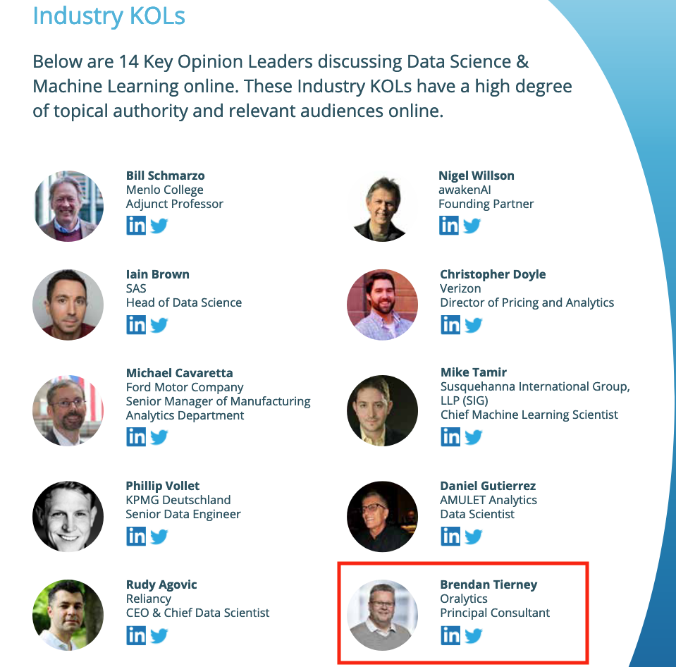
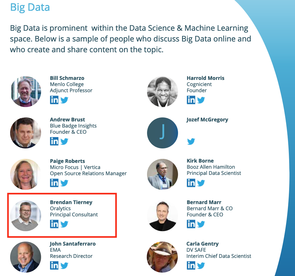
This is what Onalytica says about their report and how the list for each category was put together. “The influential experts are selected using Onalytica’s 4 Rs methodology (Reach, Resonance, Relevance and Reference). Quantitative data is pulled through LinkedIn, Twitter, Personal Blogs, YouTube, Podcast, and Forbes channels, and our qualitative data is pulled by our insights and analytics team, capturing offline influenc”. “All the influential experts featured are categorised by influencer persona, the sector they work in, their role within that sector, and more from our curated database of 1m+ influencers”. “Our Who’s Who lists are created using the Onalytica platform which has a curated database of over 1 million influencers. Our platform allows you to discover, validate and categorise influencers quickly and easily via keyword searches. Our lists are made using carefully created Boolean queries which then rank influencers by resonance, relevance, reach and reference, meaning influencers are not only ranked by themselves, but also by how much other influencers are referring to them. The lists are then validated, and filters are used to split the influencers up into the categories that are seen in the list.”
Check out the full report on “Who’s Who in Data Science & Machine Learning?“
Data Science (The MIT Press Essential Knowledge series) – available in English, Korean and Chinese
Back in the middle of 2018 MIT Press published my Data Science book, co-written with John Kelleher. It book was published as part of their Essentials Series.
During the few months it was available in 2018 it became a best seller on Amazon, and one of the top best selling books for MIT Press. This happened again in 2019. Yes, two years running it has been a best seller!
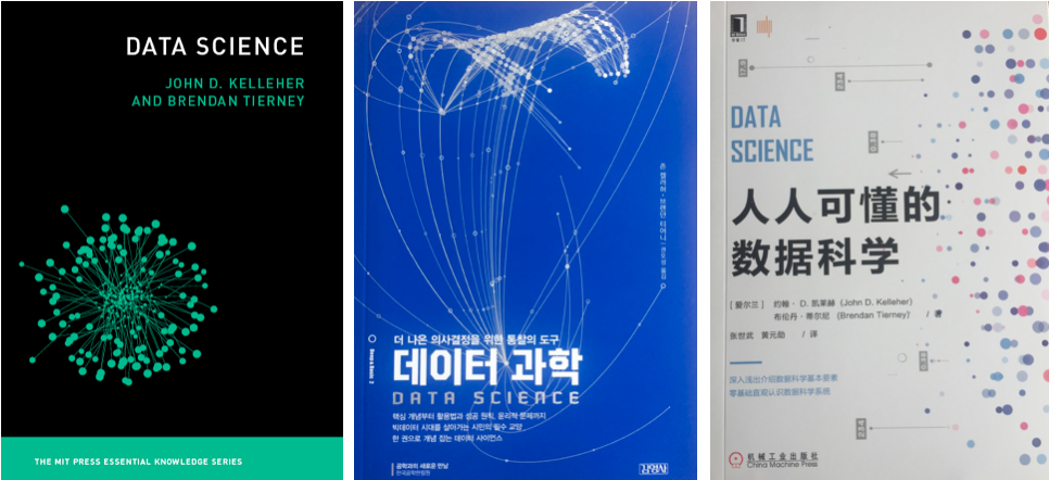
2020 kicks off with the book being translated into Korean and Chinese. Here are the covers of these translated books.


The Japanese and Turkish translations will be available in a few months!
Go get the English version of the book on Amazon in print, Kindle and Audio formats.
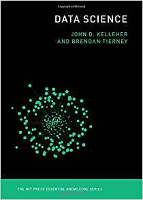
This book gives a concise introduction to the emerging field of data science, explaining its evolution, relation to machine learning, current uses, data infrastructure issues and ethical challenge the goal of data science is to improve decision making through the analysis of data. Today data science determines the ads we see online, the books and movies that are recommended to us online, which emails are filtered into our spam folders, even how much we pay for health insurance.
Go check it out.
Examples of using Machine Learning on Video and Photo in Public
Over the past 18 months or so most of the examples of using machine learning have been on looking at images and identifying objects in them. There are the typical examples of examining pictures looking for a Cat or a Dog, or some famous person, etc. Most of these examples are very noddy, although they do illustrate important examples.
But what if this same technology was used to monitor people going about their daily lives. What if pictures and/or video was captured of you as you walked down the street or on your way to work or to a meeting. These pictures and videos are being taken of you without you knowing.
And this raises a wide range of Ethical concerns. There are the ethics of deploying such solutions in the public domain, but there are also ethical concerns for the data scientists, machine learner, and other people working on these projects. “Just because we can, doesn’t mean we should”. People need to decide, if they are working on one of these projects, if they should be working on it and if not what they can do.
Ethics are the principals of behavior based on ideas of right and wrong. Ethical principles often focus on ideas such as fairness, respect, responsibility, integrity, quality, transparency and trust. There is a lot in that statement on Ethics, but we all need to consider that is right and what is wrong. But instead of wrong, what is grey-ish, borderline scenarios.
Here are some examples that might fall into the grey-ish space between right and wrong. Why they might fall more towards the wrong is because most people are not aware their image is being captured and used, not just for a particular purpose at capture time, but longer term to allow for better machine learning models to be built.
Can you imagine walking down the street with a digital display in front of you. That display is monitoring you, and others, and then presents personalized adverts on the digital display aim specifically at you. A classify example of this is in the film Minority Report. This is no longer science fiction.

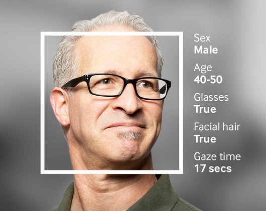
This is happening at the Westfield shopping center in London and in other cities across UK and Europe. These digital advertisement screens are monitoring people, identifying their personal characteristics and then customizing the adverts to match in with the profile of the people walking past. This solutions has been developed and rolled out by Ocean Out Door. They are using machine learning to profile the individual people based on gender, age, facial hair, eye wear, mood, engagement, attention time, group size, etc. They then use this information to:
- Optimisation – delivering the appropriate creative to the right audience at the right time.
- Visualise – Gaze recognition to trigger creative or an interactive experience
- AR Enabled – Using the HD cameras to create an augmented reality mirror or window effect, creating deep consumer engagement via the latest technology
- Analytics – Understanding your brand’s audience, post campaign analysis and creative testing
Face Plus Plus can monitor people walking down the street and do similar profiling, and can bring it to another level where by they can identify what clothing you are wearing and what the brand is. Image if you combine this with location based services. An example of this, imagine you are walking down the high street or a major retail district. People approach you trying to entice you into going into a particular store, and they offer certain discounts. But you are with a friend and the store is not interested in them.

The store is using video monitoring, capturing details of every person walking down the street and are about to pass the store. The video is using machine/deep learning to analyze you profile and what brands you are wearing. The store as a team of people who are deployed to stop and engage with certain individuals, just because they make the brands or interests of the store and depending on what brands you are wearing can offer customized discounts and offers to you.
How comfortable would you be with this? How comfortable would you be about going shopping now?
For me, I would not like this at all, but I can understand why store and retail outlets are interested, as they are all working in a very competitive market trying to maximize every dollar or euro they can get.
Along side the ethical concerns, we also have some legal aspects to consider. Some of these are a bit in the grey-ish area, as some aspects of these kind of scenarios are slightly addresses by EU GDPR and the EU Artificial Intelligence guidelines. But what about other countries around the World. Then it comes to training and deploying these facial models, they are dependent on having a good training data set. This means they needs lots and lots of pictures of people and these pictures need to be labelled with descriptive information about the person. For these public deployments of facial recognition systems, then will need more and more training samples/pictures. This will allow the models to improve and evolve over time. But how will these applications get these new pictures? They claim they don’t keep any of the images of people. They only take the picture, use the model on it, and then perform some action. They claim they do not keep the images! But how can they improve and evolve their solution?
I’ll have another blog post giving more examples of how machine/deep learning, video and image captures are being used to monitor people going about their daily lives.
Ethics in the AI, Machine Learning, Data Science, etc Era
Ethics is one of those topics that everyone has a slightly different definition or view of what it means. The Oxford English dictionary defines ethics as, ‘Moral principles that govern a person’s behaviour or the conducting of an activity‘.
As you can imagine this topic can be difficult to discuss and has many, many different aspects.
In the era of AI, Machine Learning, Data Science, etc the topic of Ethics is finally becoming an important topic. Again there are many perspective on this. I’m not going to get into these in this blog post, because if I did I could end up writing a PhD dissertation on it.
But if you do work in the area of AI, Machine Learning, Data Science, etc you do need to think about the ethical aspects of what you do. For most people, you will be working on topics where ethics doesn’t really apply. For example, examining log data, looking for trends, etc
But when you start working of projects examining individuals and their behaviours then you do need to examine the ethical aspects of such work. Everyday we experience adverts, web sites, marketing, etc that has used AI, Machine Learning and Data Science to delivery certain product offerings to us.
Just because we can do something, doesn’t mean we should do it.

One particular area that I will not work on is Location Based Advertising. Imagine walking down a typical high street with lots and lots of retail stores. Your phone vibrates and on the screen there is a message. The message is a special offer or promotion for one of the shops a short distance ahead of you. You are being analysed. Your previous buying patterns and behaviours are being analysed, Your location and direction of travel is being analysed. Some one, or many AI applications are watching you. This is not anything new and there are lots of examples of this from around the world.

But what if this kind of Location Based Advertising was taken to another level. What if the shops had cameras that monitored the people walking up and down the street. What if those cameras were analysing you, analysing what clothes you are wearing, analysing the brands you are wearing, analysing what accessories you have, analysing your body language, etc. They are trying to analyse if you are the kind of person they want to sell to. They then have staff who will come up to you, as you are walking down the street, and will have customised personalised special offers on products in their store, just for you.
See the segment between 2:00 and 4:00 in this video. This gives you an idea of what is possible.
Are you Ok with this?
As an AI, Machine Learning, Data Science professional, are you Ok with this?
The technology exists to make this kind of Location Based Marketing possible. This will be an increasing ethical consideration over the coming years for those who work in the area of AI, Machine Learning, Data Science, etc
Just because we can, doesn’t mean we should!
Lessor known Apache Machine Learning Languages
Machine learning is a very popular topic in recent times, and we keep hearing about languages such as R, Python and Spark. In addition to these we have commercially available machine learning languages and tools from SAS, IBM, Microsoft, Oracle, Google, Amazon, etc., etc. Everyone want a slice of the machine learning market!
The Apache Foundation supports the development of new open source projects in a number of areas. One such area is machine learning. If you have read anything about machine learning you will have come across Spark, and maybe you might believe that everyone is using it. Sadly this isn’t true for lots of reasons, but it is very popular. Spark is one of the project support by the Apache Foundation.
But are there any other machine learning projects being supported under the Apache Foundation that are an alternative to Spark? The follow lists the alternatives and lessor know projects: (most of these are incubator/retired/graduated Apache projects)
| Flink | Flink is an open source system for expressive, declarative, fast, and efficient data analysis. Stratosphere combines the scalability and programming flexibility of distributed MapReduce-like platforms with the efficiency, out-of-core execution, and query optimization capabilities found in parallel databases. Flink was originally known as Stratosphere when it entered the Incubator.
(graduated) |
| HORN | HORN is a neuron-centric programming APIs and execution framework for large-scale deep learning, built on top of Apache Hama.
(Retired) |
| HiveMail | Hivemall is a library for machine learning implemented as Hive UDFs/UDAFs/UDTFs
Apache Hivemall offers a variety of functionalities: regression, classification, recommendation, anomaly detection, k-nearest neighbor, and feature engineering. It also supports state-of-the-art machine learning algorithms such as Soft Confidence Weighted, Adaptive Regularization of Weight Vectors, Factorization Machines, and AdaDelta. Apache Hivemall offers a variety of functionalities: regression, classification, recommendation, anomaly detection, k-nearest neighbor, and feature engineering. It also supports state-of-the-art machine learning algorithms such as Soft Confidence Weighted, Adaptive Regularization of Weight Vectors, Factorization Machines, and AdaDelta. (incubator) |
| MADlib | Apache MADlib is an open-source library for scalable in-database analytics. It provides data-parallel implementations of mathematical, statistical and machine learning methods for structured and unstructured data. Key features include: Operate on the data locally in-database. Do not move data between multiple runtime environments unnecessarily; Utilize best of breed database engines, but separate the machine learning logic from database specific implementation details; Leverage MPP shared nothing technology, such as the Greenplum Database and Apache HAWQ (incubating), to provide parallelism and scalability.
(graduated) |
| MXNet | A Flexible and Efficient Library for Deep Learning . MXNet provides optimized numerical computation for GPUs and distributed ecosystems, from the comfort of high-level environments like Python and R MXNet automates common workflows, so standard neural networks can be expressed concisely in just a few lines of code.
(incubator) |
| OpenNLP | OpenNLP is a machine learning based toolkit for the processing of natural language text. OpenNLP supports the most common NLP tasks, such as tokenization, sentence segmentation, part-of-speech tagging, named entity extraction, chunking, parsing, language detection and coreference resolution.
(graduated) |
| PredictionIO | PredictionIO is an open source Machine Learning Server built on top of state-of-the-art open source stack, that enables developers to manage and deploy production-ready predictive services for various kinds of machine learning tasks.
(graduated) |
| SAMOA | SAMOA provides a collection of distributed streaming algorithms for the most common data mining and machine learning tasks such as classification, clustering, and regression, as well as programming abstractions to develop new algorithms that run on top of distributed stream processing engines (DSPEs). It features a pluggable architecture that allows it to run on several DSPEs such as Apache Storm, Apache S4, and Apache Samza.
(incubator) |
| SINGA | SINGA is a distributed deep learning platform. An intuitive programming model based on the layer abstraction is provided, which supports a variety of popular deep learning models. SINGA architecture supports both synchronous and asynchronous training frameworks. Hybrid training frameworks can also be customized to achieve good scalability. SINGA provides different neural net partitioning schemes for training large models.
(incubator) |
| Storm | Storm is a distributed, fault-tolerant, and high-performance realtime computation system that provides strong guarantees on the processing of data. Storm makes it easy to reliably process unbounded streams of data, doing for realtime processing what Hadoop did for batch processing. Storm is simple, can be used with any programming language.
(graduated) |
| SystemML | SystemML provides declarative large-scale machine learning (ML) that aims at flexible specification of ML algorithms and automatic generation of hybrid runtime plans ranging from single node, in-memory computations, to distributed computations such as Apache Hadoop MapReduce and Apache Spark.
(graduated) |

I will have a closer look that the following SQL based machine learning languages in a lager blog post:
– MADlib
– Storm

You must be logged in to post a comment.