
Machine Learning
Why Choose Apache Iceberg for Data Interoperability?
Modern data platforms increasingly separate compute from storage, using object stores as durable data lakes while scaling processing engines. Traditional “data lakes” built on Parquet files and Hive-style partitioning have limitations around atomicity, schema evolution, metadata scalability, and multi-engine interoperability. Apache Iceberg addresses these challenges by defining a high-performance table format with transactional guarantees, scalable metadata structures, and engine-agnostic semantics.
Apache Iceberg, an open-source table format that has become the industry standard for data sharing in modern data architectures. Let’s have a look at some of the key features, some of its limitations and a brief look at some of the alternatives.
What is Apache Iceberg and Why Do We Need It? Apache Iceberg is not a storage engine or a compute engine; it’s a table format. It acts as a metadata layer that sits between your physical data files (Parquet, ORC, Avro) and your compute engines.
Before Iceberg, data lakes managed tables as directories of files. To find data, an engine had to list all files in a directory—a slow operation on cloud storage. There was no guarantee of data consistency; a reader might see a partially written file from a running job. Iceberg solves this by tracking individual data files in a persistent tree of metadata. This effectively brings semi-database level reliability, with ACID transactions and snapshot isolation, together with the flexible, low-cost world of object storage.
Iceberg has several important features that bridge the gap between data lakes and traditional warehouses like Oracle:
- ACID Transactions: Iceberg ensures that readers never see partial or uncommitted data. Every write operation creates a new, immutable snapshot. Commits are atomic, meaning they either fully succeed or fully fail. This is the same level of integrity that database administrators have come to expect from Oracle Database for decades.
- Reliable Schema Evolution: In the past, adding or renaming a column in a data lake could require a complete rewrite of your data. Iceberg supports full schema evolution—adding, dropping, updating, or renaming columns—as a metadata operation. It ensures that “zombie” data or schema mismatches never crash your production pipelines.
- Hidden Partitioning: This is a massive usability improvement. Instead of forcing users to know the physical directory structure (e.g.,
WHERE year=2026), Iceberg handles partitioning transparently. You can partition by a timestamp, and Iceberg handles the logic. This makes the data lake feel more like a standard SQL table in a relational Database, where the physical storage details are abstracted away from the analyst. - Time Travel and Rollback: Because Iceberg maintains a history of table snapshots, you can query the data as it existed at any point in history. This is invaluable for auditing, reproducing machine learning models, or quickly rolling back accidental bad writes without needing to restore from a massive tape backup.
While the benefits of Apache Iceberg Tables are critical for its adaption, there are also some limitations:
- Metadata Overhead: The metadata layer adds complexity. For extremely small, high-frequency “single-row” writes, the overhead of managing metadata files can be significant compared to a highly tuned RDBMS.
- Tooling Maturity: While major players like AWS, Snowflake, Oracle, etc have adopted it, support across the entire data ecosystem is still evolving. You may occasionally encounter older tools that don’t natively understand Iceberg tables.
- Write Latency: Every commit involves writing new manifest and metadata files. While this is fine for batch and micro-batch processing, it may not replace the sub-second latency required for OLTP (Online Transactional Processing) workloads where relational Database still reign supreme.
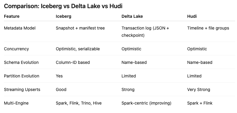
Alternatives to Apache Iceberg tables include Delta Lake (from Databricks) and Apache Hudi. While Delta Lake is highly optimized for the Spark ecosystem and offers a rich feature set, its governance has historically been closely tied to Databricks. Apache Hudi is optimized in streaming ingestion and near-real-time upsert use cases due to its unique indexing and log-merge capabilities. etc it can take some time to consolidate the data change logs. Apache Iceberg is often the choice for organizations seeking maximum interoperability. Its design allows diverse engines, from Spark and Trino to Snowflake and Oracle, to interact with the same data without vendor lock-in and with minimum data copying.
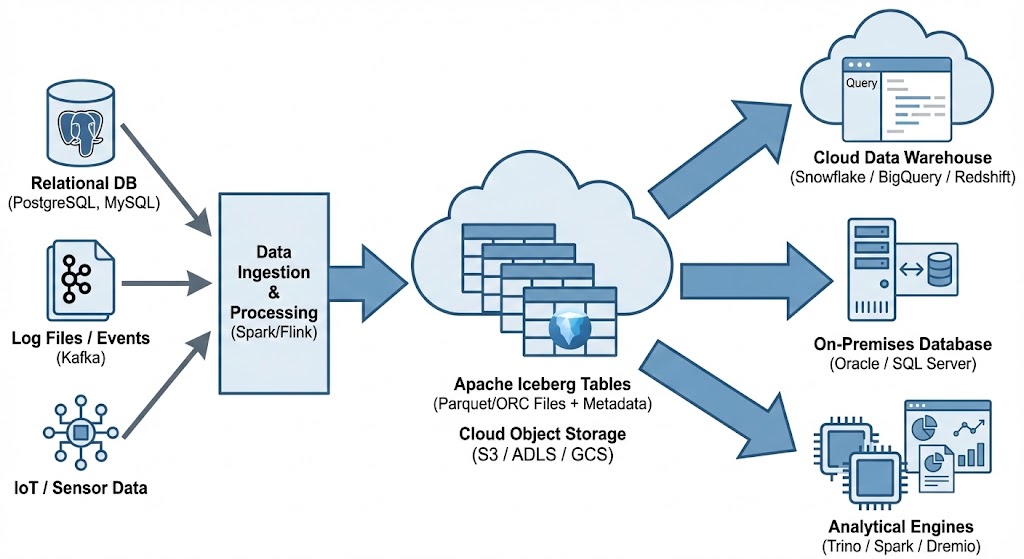
One of Apache Iceberg’s greatest strengths is its ability to act as a central, interoperable layer for data sharing across different platforms. By standardizing on Iceberg, you break down silos. Data ingested once into your data lake becomes immediately available to multiple consuming systems without complex ETL pipelines. Data from various sources is ingested and stored as Apache Iceberg tables in cloud object storage. From there, it can be seamlessly queried by cloud data warehouses like Snowflake and Oracle, etc, and synced to on-premises databases, like Oracle and others, or accessed by various analytical engines for BI and data science.
Creating Test Data in your Database using Faker
A some point everyone needs some test data for their database. There area a number of ways of doing this, and in this post I’ll walk through using the Python library Faker to create some dummy test data (that kind of looks real) in my Oracle Database. I’ll have another post using the GenAI in-database feature available in the Oracle Autonomous Database. So keep an eye out for that.
Faker is one of the available libraries in Python for creating dummy/test data that kind of looks realistic. There are several more. I’m not going to get into the relative advantages and disadvantages of each, so I’ll leave that task to yourself. I’m just going to give you a quick demonstration of what is possible.
One of the key elements of using Faker is that we can set a geograpic location for the data to be generated. We can also set multiples of these and by setting this we can get data generated specific for that/those particular geographic locations. This is useful for when testing applications for different potential markets. In my example below I’m setting my local for USA (en_US).
Here’s the Python code to generate the Test Data with 15,000 records, which I also save to a CSV file.
import pandas as pd
from faker import Faker
import random
from datetime import date, timedelta

#####################
NUM_RECORDS = 15000
LOCALE = 'en_US'

#Initialise Faker
Faker.seed(42)
fake = Faker(LOCALE)

#####################

#Create a function to generate the data
def create_customer_record():
    #Customer Gender
    gender = random.choice(['Male', 'Female', 'Non-Binary'])
    #Customer Name
    if gender == 'Male':
        name = fake.name_male()
    elif gender == 'Female':
        name = fake.name_female()
    else:
        name = fake.name()

    #Date of Birth
    dob = fake.date_of_birth(minimum_age=18, maximum_age=90)

    #Customer Address and other details
    address = fake.street_address()
    email = fake.email()
    city = fake.city()
    state = fake.state_abbr()
    zip_code = fake.postcode()
    full_address = f"{address}, {city}, {state} {zip_code}"
    phone_number = fake.phone_number()

    #Customer Income
    #  - annual income between $30,000 and $250,000
    income = random.randint(300, 2500) * 100

    #Credit Rating
    credit_rating = random.choices(['A', 'B', 'C', 'D'], weights=[0.40, 0.30, 0.20, 0.10], k=1)[0]

    #Credit Card and Banking details
    card_type = random.choice(['visa', 'mastercard', 'amex'])
    credit_card_number = fake.credit_card_number(card_type=card_type)
    routing_number = fake.aba()
    bank_account = fake.bban()

    return {
        'CUSTOMERID': fake.unique.uuid4(), # Unique identifier
        'CUSTOMERNAME': name,
        'GENDER': gender,
        'EMAIL': email,
        'DATEOFBIRTH': dob.strftime('%Y-%m-%d'),
        'ANNUALINCOME': income,
        'CREDITRATING': credit_rating,
        'CUSTOMERADDRESS': full_address,
        'ZIPCODE': zip_code,
        'PHONENUMBER': phone_number,
        'CREDITCARDTYPE': card_type.capitalize(),
        'CREDITCARDNUMBER': credit_card_number,
        'BANKACCOUNTNUMBER': bank_account,
        'ROUTINGNUMBER': routing_number,
    }

#Generate the Demo Data
print(f"Generating {NUM_RECORDS} customer records...")
data = [create_customer_record() for _ in range(NUM_RECORDS)]
print("Sample Data Generation complete")

#Convert to Pandas DataFrame
df = pd.DataFrame(data)

print("\n--- DataFrame Sample (First 10 Rows) : sample of columns ---")
# Display relevant columns for verification
display_cols = ['CUSTOMERNAME', 'GENDER', 'DATEOFBIRTH', 'PHONENUMBER', 'CREDITCARDNUMBER', 'CREDITRATING', 'ZIPCODE']
print(df[display_cols].head(10).to_markdown(index=False))

print("\n--- DataFrame Information ---")
print(f"Total Rows: {len(df)}")
print(f"Total Columns: {len(df.columns)}")
print("Data Types:")
print(df.dtypes)
The output from the above code gives the following:
Generating 15000 customer records...
Sample Data Generation complete

--- DataFrame Sample (First 10 Rows) : sample of columns ---
| CUSTOMERNAME     | GENDER     | DATEOFBIRTH   | PHONENUMBER            |   CREDITCARDNUMBER | CREDITRATING   |   ZIPCODE |
|:-----------------|:-----------|:--------------|:-----------------------|-------------------:|:---------------|----------:|
| Allison Hill     | Non-Binary | 1951-03-02    | 479.540.2654           |   2271161559407810 | A              |     55488 |
| Mark Ferguson    | Non-Binary | 1952-09-28    | 724.523.8849x696       |    348710122691665 | A              |     84760 |
| Kimberly Osborne | Female     | 1973-08-02    | 001-822-778-2489x63834 |   4871331509839301 | B              |     70323 |
| Amy Valdez       | Female     | 1982-01-16    | +1-880-213-2677x3602   |   4474687234309808 | B              |     07131 |
| Eugene Green     | Male       | 1983-10-05    | (442)678-4980x841      |   4182449353487409 | A              |     32519 |
| Timothy Stanton  | Non-Binary | 1937-10-13    | (707)633-7543x3036     |    344586850142947 | A              |     14669 |
| Eric Parker      | Male       | 1964-09-06    | 577-673-8721x48951     |   2243200379176935 | C              |     86314 |
| Lisa Ball        | Non-Binary | 1971-09-20    | 516.865.8760           |    379096705466887 | A              |     93092 |
| Garrett Gibson   | Male       | 1959-07-05    | 001-437-645-2991       |    349049663193149 | A              |     15494 |
| John Petersen    | Male       | 1978-02-14    | 367.683.7770           |   2246349578856859 | A              |     11722 |

--- DataFrame Information ---
Total Rows: 15000
Total Columns: 14
Data Types:
CUSTOMERID           object
CUSTOMERNAME         object
GENDER               object
EMAIL                object
DATEOFBIRTH          object
ANNUALINCOME          int64
CREDITRATING         object
CUSTOMERADDRESS      object
ZIPCODE              object
PHONENUMBER          object
CREDITCARDTYPE       object
CREDITCARDNUMBER     object
BANKACCOUNTNUMBER    object
ROUTINGNUMBER        object
Having generated the Test data, we now need to get it into the database. There a various ways of doing this. As we are already using Python I’ll illustrate getting the data into the Database below. An alternative option is to use SQL Command Line (SQLcl) and the LOAD feature in that tool.
Here’s the Python code to load the data. I’m using the oracledb python library.
### Connect to Database
import oracledb

p_username = "..."
p_password = "..."

#Give OCI Wallet location and details
try:
    con = oracledb.connect(user=p_username, password=p_password, dsn="adb26ai_high",
                       config_dir="/Users/brendan.tierney/Dropbox/Wallet_ADB26ai",
                       wallet_location="/Users/brendan.tierney/Dropbox/Wallet_ADB26ai",
                       wallet_password=p_walletpass)
except Exception as e:
    print('Error connecting to the Database')
    print(f'Error:{e}')

print(con)
### Create Customer Table
drop_table = 'DROP TABLE IF EXISTS demo_customer'
cre_table = '''CREATE TABLE DEMO_CUSTOMER (
CustomerID VARCHAR2(50) PRIMARY KEY,
CustomerName VARCHAR2(50),
Gender VARCHAR2(10),
Email VARCHAR2(50),
DateOfBirth DATE,
AnnualIncome NUMBER(10,2),
CreditRating VARCHAR2(1),
CustomerAddress VARCHAR2(100),
ZipCode VARCHAR2(10),
PhoneNumber VARCHAR2(50),
CreditCardType VARCHAR2(10),
CreditCardNumber VARCHAR2(30),
BankAccountNumber VARCHAR2(30),
RoutingNumber VARCHAR2(10) )'''
cur = con.cursor()
print('--- Dropping DEMO_CUSTOMER table ---')
cur.execute(drop_table)
print('--- Creating DEMO_CUSTOMER table ---')
cur.execute(cre_table)
print('--- Table Created ---')### Insert Data into Table
insert_data = '''INSERT INTO DEMO_CUSTOMER values (:1, :2, :3, :4, :5, :6, :7, :8, :9, :10, :11, :12, :13, :14)'''
print("--- Inserting records ---")
cur.executemany(insert_data, df )
con.commit()
print("--- Saving to CSV ---")
df.to_csv('/Users/brendan.tierney/Dropbox/DEMO_Customer_data.csv', index=False)
print("- Finished -")### Close Connections to DB
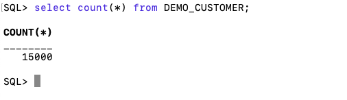
con.close()and to prove the records got inserted we can connect to the schema using SQLcl and check.
Where to find Blogs on Oracle Database
A regular question I get asked is, “is there a list of Oracle-related Blogs?” and “what people/blogs should I follow to learn more about Oracle Database?” This typically gets asked by people in the early stages of their careers and even by those who have been around for a while.
You could ask these questions to twenty different (experienced) people, and you’d get largely the same answers with some variations. These variations would be down to their preferences on how certain people cover certain topics. This comes down to experience of following lots of people and learning over time.
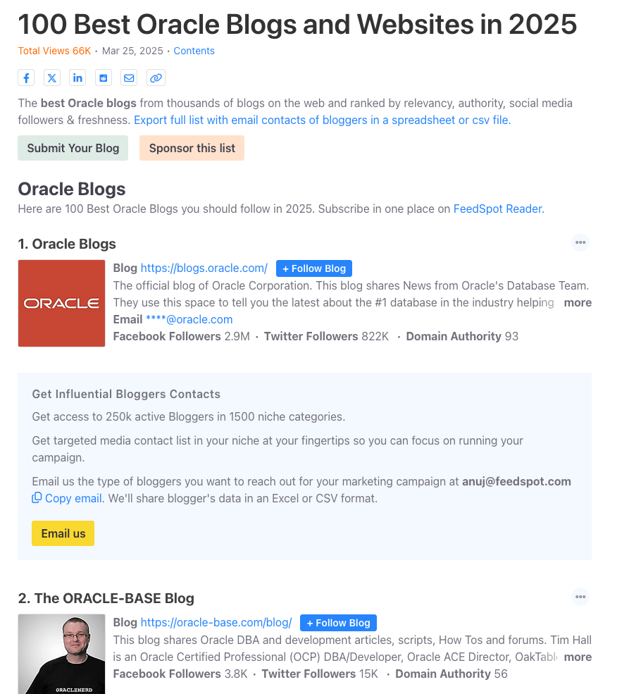
But where can people get started quickly with a list of 100 blogs. Feedspot is one such place where you can find such a place and subscribe for update emails when new blog posts are written.
Go check out the list. You might discover some new bloggers and content.
Using Cohere to Generate Vector Embeddings
When using Vector Databases or Vector Embedding features in most (modern, multi-model) Databases, you can gain additional insights. The Vector Embeddings can be utilised for semantic searches, where you can find related data or information based on the values of the Vectors. One of the challenges is generating suitable vectors. There are a lot of options available for generating these Vector Embeddings. In this post, I’ll illustrate how to generate these using Cohere, and in a future post, I’ll illustrate using OpenAI. There are advantages and disadvantages to using these solutions. I’ll point out some of these for each solution (Cohere and OpenAI), using their Python API library.
The first step is to install the Cohere Python library
pip install cohereNext, you need to create an account with Cohere. This will allow you to get an API key. You can get a Trial API key, but you will be restricted to the number of calls you are allowed. As with most free or trial keys these allow you to do a limited number of calls. This is commonly referred to as Rate Limiting. The trial key for the embedding models allows you to have up to 40 calls per minute. This is very very limited and each call is very slow. (I’ll discuss related issues about OpenAI rate limiting in another post)
The dataset I’ll be using is the Wine Reviews 130K (dropbox link). This is widely available on many sites. I want to create Vector Embeddings for the ‘Description’ field in this dataset which contains a review of each wine. There are some columns with no values, and these need to be handled. For each wine review, I’ll create a SQL INSERT statement and print this out to a file. This file will contain an INSERT statement for each wine review, including the vector embedding.
Here’s the code, (you’ll need to enter an API key and change the directory for the data file)
import numpy as np
import os
import time
import pandas as pd
import cohere

co = cohere.Client(api_key="...")

data_file = ".../VectorDatabase/winemag-data-130k-v2.csv"
df = pd.read_csv(data_file)

print_every = 200
rate_limit = 1000 #Cohere limits to 40 API calls per minute

print("Input file :", data_file)
v_file = os.path.splitext(data_file)[0]+'.cohere'
print(v_file)

#Open file with write (over-writes previous file)
f=open(v_file,"w")
for index,row in df.head(rate_limit).iterrows():
    phrases=list(row['description'])
    model="embed-english-v3.0"
    input_type="search_query"
    #####
    res = co.embed(texts=phrases,
                model=model,
                input_type=input_type) #,
#                embedding_types=['float'])

    v_embedding = str(res.embeddings[0])
    tab_insert="INSERT into WINE_REVIEWS_130K VALUES ("+str(row["Seq"])+"," \
        +'"'+str(row["description"])+'",' \
        +'"'+str(row["designation"])+'",' \
        +str(row["points"])+"," \
        +'"'+str(row["province"])+'",' \
        +str(row["price"])+"," \
        +'"'+str(row["region_1"])+'",' \
        +'"'+str(row["region_2"])+'",' \
        +'"'+str(row["taster_name"])+'",' \
        +'"'+str(row["taster_twitter_handle"])+'",' \
        +'"'+str(row["title"])+'",' \
        +'"'+str(row["variety"])+'",' \
        +'"'+str(row["winery"])+'",' \
        +"'"+v_embedding+"'"+");\n"

    f.write(tab_insert)
    if (index%print_every == 0):
        print(f'Processed {index} vectors ', time.strftime("%H:%M:%S", time.localtime()))

#Close vector file
f.close()
print(f"Finished writing file with Vector data [{index+1} vectors]", time.strftime("%H:%M:%S", time.localtime()))
The vector generated has 1024 dimensions. At this time there isn’t a parameter to change/reduce the number of dimensions.
The output file can now be run in your database, assuming you’ve created a table called WINE_REVIEWS_130K and has a column with the appropriate data type (e.g. VECTOR)
Warnings: When using the Cohere API you are limited to maximum of 40 calls per minute. I’ve found this to be incorrect and it was more like 38 calls (for me). I also found the ‘per minute’ to be incorrect. I had to wait several minutes and up to five minutes before I could attempt another run.
In an attempt to overcome this, I create a production API key. This involved giving some payment details, and this in theory should remove the ‘per minute’ rate limit, among other things. Unfortunately, for me this was not a good experience, as I had to make multiple attempts to run for 1000 records before I could have a successful outcome. I experienced multiple Server 500 errors and other errors that related to Cohere server problems.
I wasn’t able to process more that 600 records before the errors occurred and I wasn’t able to generate for a larger percentage of the dataset.
An additional issue is with the response time from Cohere. It was taking approx. 5 minutes to process 200 API calls.
So overall a rather poor experience. I then switched to OpenAI and had a slightly different experience. Check out that post for more details.
EU AI Act: Key Dates and Impact on AI Developers
The official text of the EU AI Act has been published in the EU Journal. This is another landmark point for the EU AI Act, as these regulations are set to enter into force on 1st August 2024. If you haven’t started your preparations for this, you really need to start now. See the timeline for the different stages of the EU AI Act below.
The EU AI Act is a landmark piece of legislation and similar legislation is being drafted/enacted in various geographic regions around the world. The EU AI Act is considered the most extensive legal framework for AI developers, deployers, importers, etc and aims to ensure AI systems introduced or currently being used in the EU internal market (even if they are developed and located outside of the EU) are secure, compliant with existing and new laws on fundamental rights and align with EU principles.
The key dates are:
- 2 February 2025: Prohibitions on Unacceptable Risk AI
- 2 August 2025: Obligations come into effect for providers of general purpose AI models. Appointment of member state competent authorities. Annual Commission review of and possible legislative amendments to the list of prohibited AI.
- 2 February 2026: Commission implements act on post market monitoring
- 2 August 2026: Obligations go into effect for high-risk AI systems specifically listed in Annex III, including systems in biometrics, critical infrastructure, education, employment, access to essential public services, law enforcement, immigration and administration of justice. Member states to have implemented rules on penalties, including administrative fines. Member state authorities to have established at least one operational AI regulatory sandbox. Commission review, and possible amendment of, the list of high-risk AI systems.
- 2 August 2027: Obligations go into effect for high-risk AI systems not prescribed in Annex III but intended to be used as a safety component of a product. Obligations go into effect for high-risk AI systems in which the AI itself is a product and the product is required to undergo a third-party conformity assessment under existing specific EU laws, for example, toys, radio equipment, in vitro diagnostic medical devices, civil aviation security and agricultural vehicles.
- By End of 2030: Obligations go into effect for certain AI systems that are components of the large-scale information technology systems established by EU law in the areas of freedom, security and justice, such as the Schengen Information System.
Here is the link to the official text in the EU Journal publication.

OCI Vision – Image model based on Object Detection
If you look back over recent blog posts you’ll see I’ve posted a few on using OCI Vision for image processing, image classification and object detection. This is another post to the series and looks to build an object detection model for images. In a previous post, I showed how to prepare an image dataset using OCI Data Labeling and using the bounding box method to outline particular objects in the image. In my examples, this involved drawing a bounding box around a Cat or a Dog in an image. After doing that the next step is to create an object detection model in OCI Vision and to test to see how well it works.
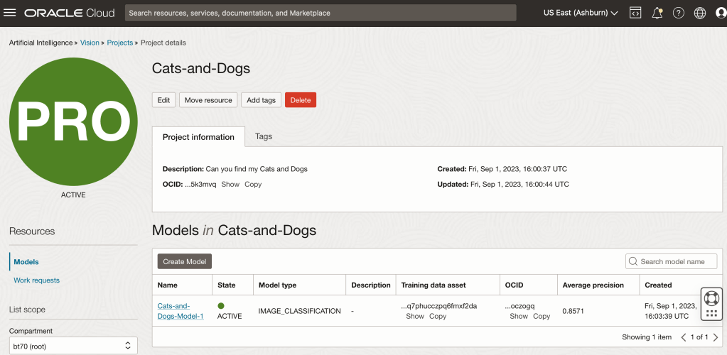
Let’s start with the OCI Vision project I created previously (see previous post).
We can add a new model to this existing project. Click on the Create Model button
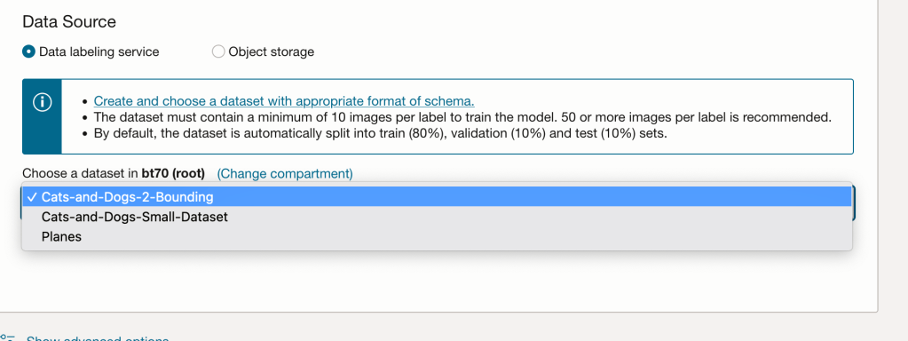
In the Create and Train model setup, select the newly defined dataset setup for object detection using bounding boxes. Then Create the model.
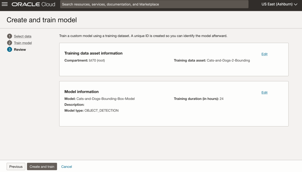
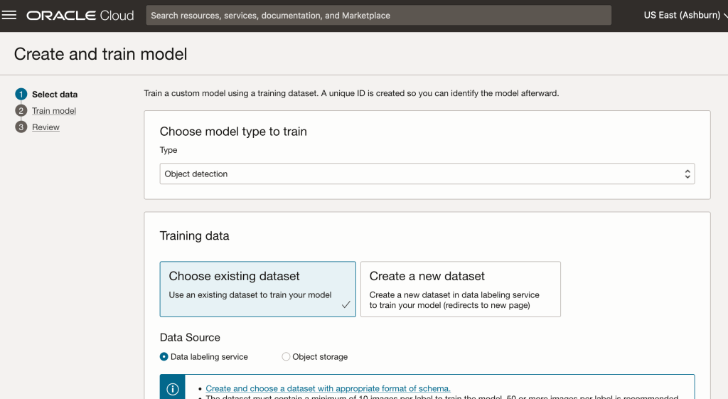
For my model, I selected the option to run for a maximum of 24 hours. It didn’t take that long and was finished in a little over an hour. The dataset is small as it only consists of 100 images.

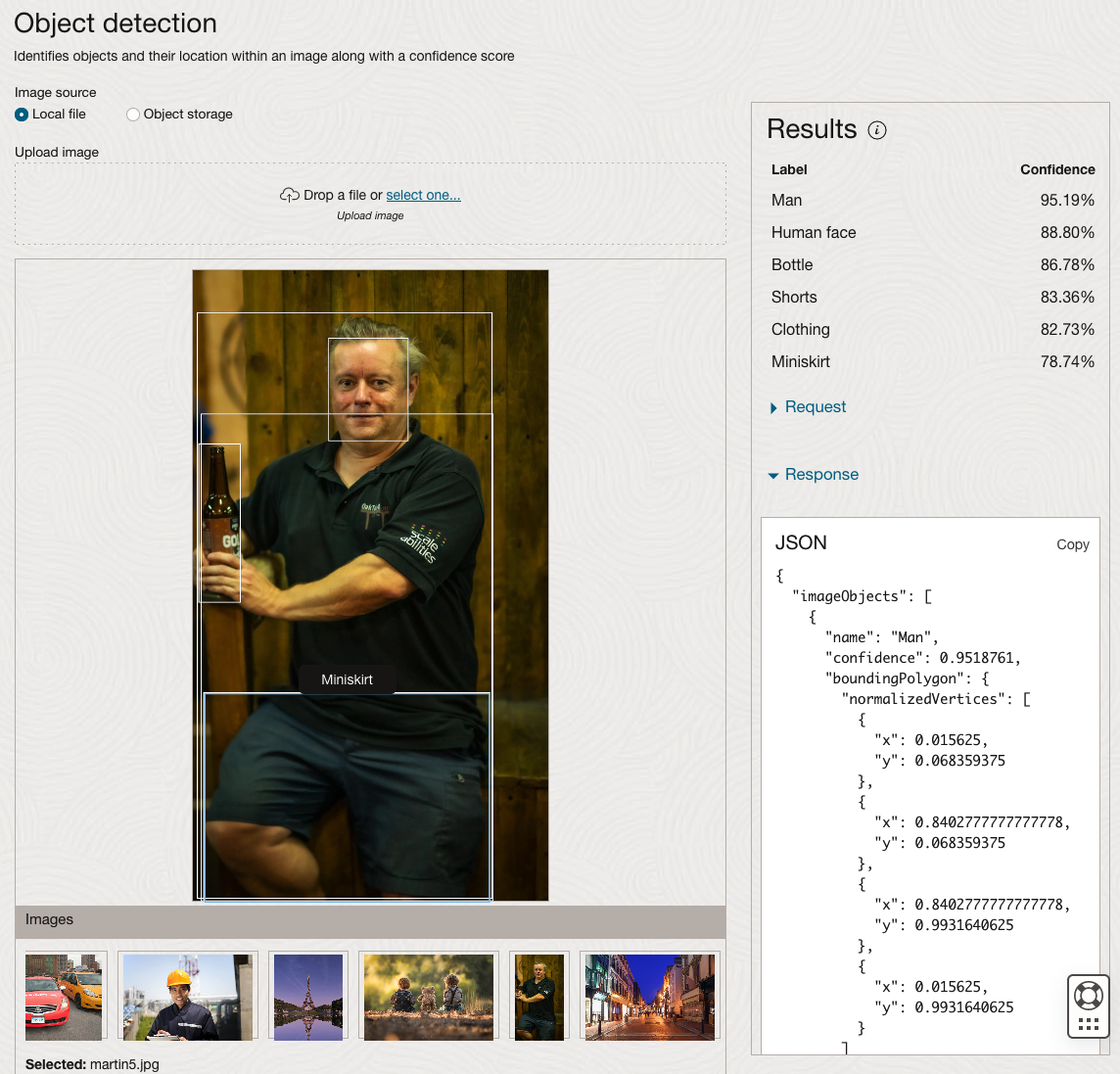
After the model was created, click into the model to view the details. This screen also allows you to upload images. The model will be applied to the images and any objects will be identified on the image and the label displayed to the right of the image. Here are a few of the images used to evaluate and these are the same images used to evaluate the previously created image classification model.
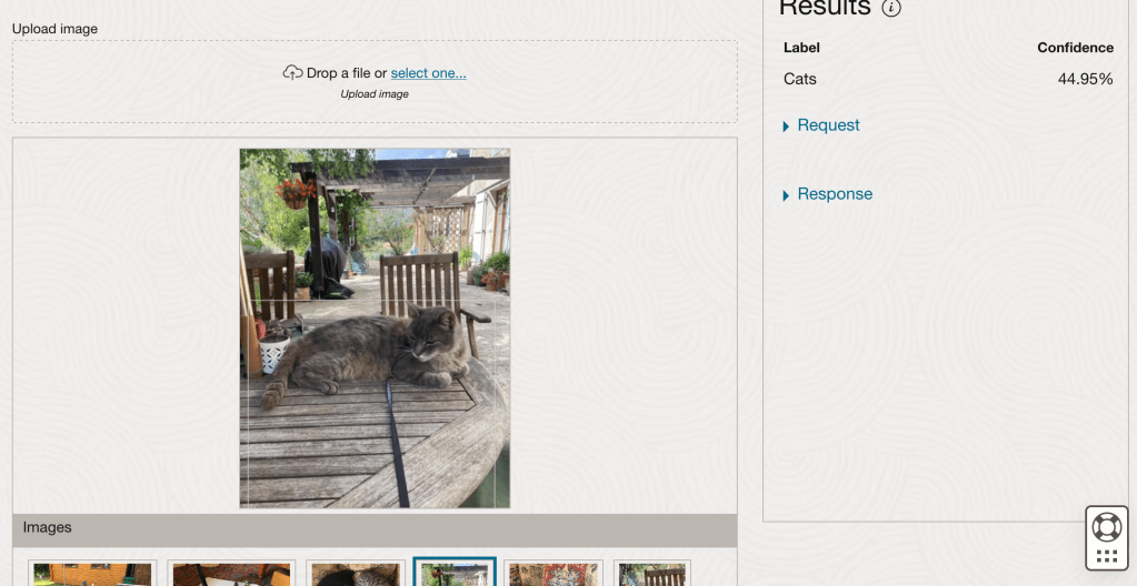
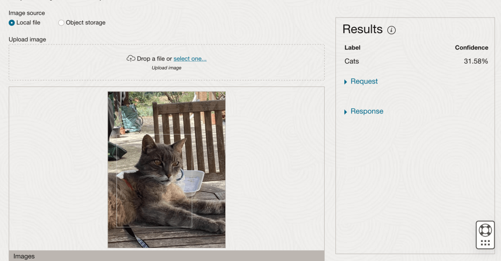
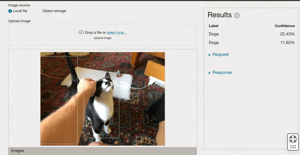
If you look closely at these images we can see the object box drawn on the images. For the image on the right, we can see there are two boxes drawn, one for the front part of the cat, then for the tail of the cat. I
OCI Vision – Creating a Custom Model for Cats and Dogs
In this post, I’ll build on the previous work on preparing data, to using this dataset as input to building a Custom AI Vision model. In the previous post, the dataset was labelled into images containing Cats and Dogs. The following steps takes you through creating the Customer AI Vision model and to test this model using some different images of Cats.
Open the OCI Vision page. On the bottom left-hand side of the menu you will see Projects. Click on this to open the Projects page for creating a Custom AI Vision model.
On the Create Projects page, click on the Create Project button. A pop-up window will appear. Enter the name for the model and click on the Create Project bottom at the bottom of the pop-up.
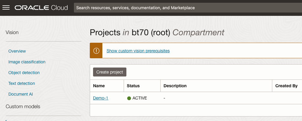
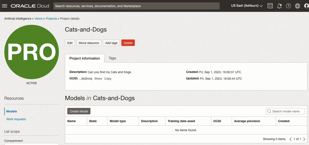
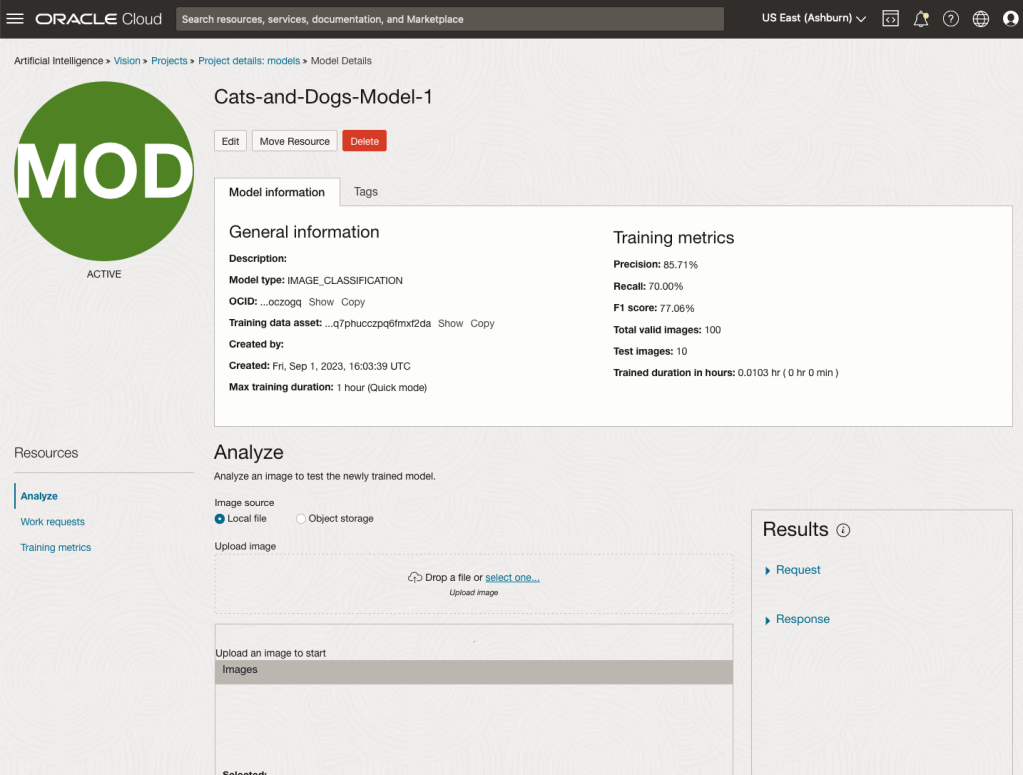
After the Project has been created, click on the project name from the list. This will open the Project specific page. A project can contain multiple models and they will be listed here. For the Cats-and-Dogs project we and to create our model. Click on the Create Model button.
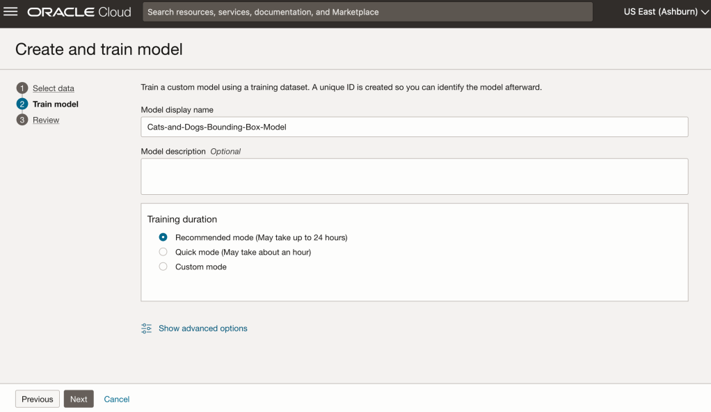
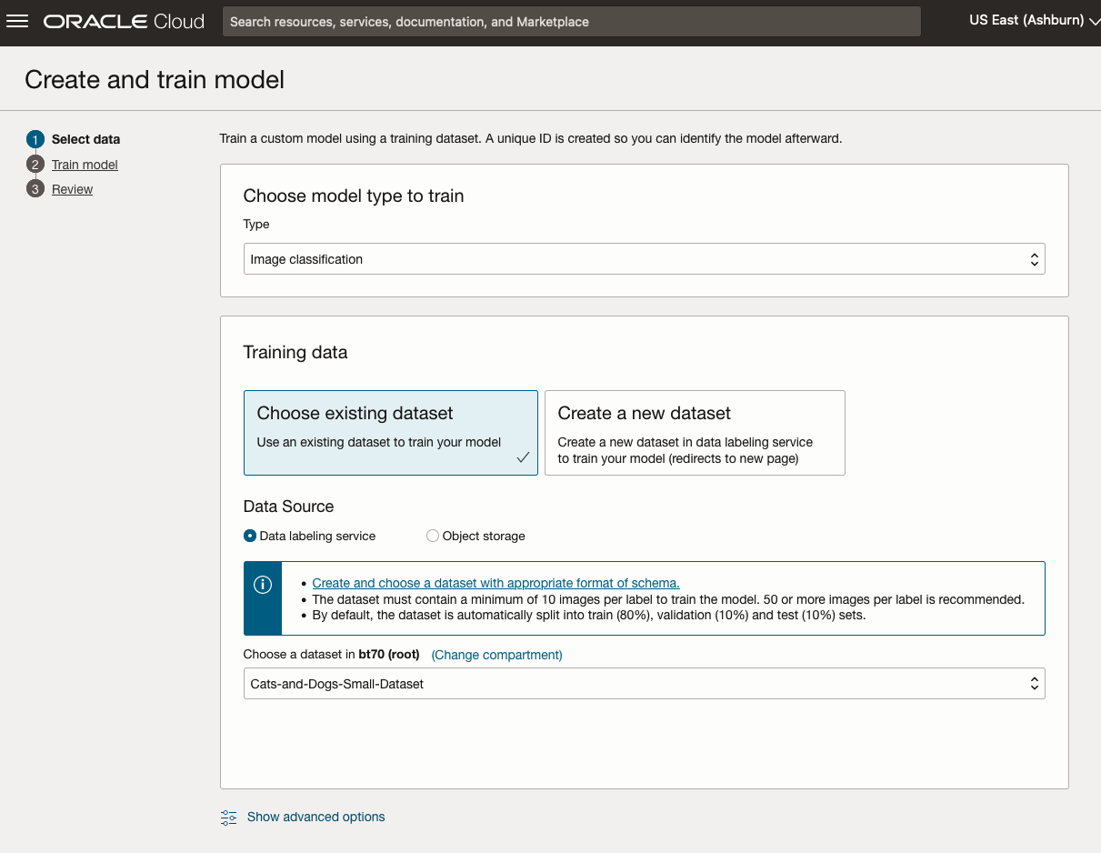
Next, you can define some of the settings for the Model. These include what dataset to use, or upload a new one, define what data labelling to use and the training duration. For this later setting, you can decide how much time you’d like to allocate to creating the custom model. Maybe consider selecting Quick mode, as that will give you a model within a few minutes (or up to an hour), whereas the other options can allow the model process to run for longer and hopefully those will create a more accurate model. As with all machine learning type models, you need to take some time to test which configuration works best for your scenario. In the following, the Quick mode option is selected. When read, click Create Model.

It can take a little bit of time to create the model. We selected the Quick mode, which has a maximum of one hour. In my scenario, the model build process was completed after four minutes. The Precentage Complete is updated during the build allowing you to monitor it’s progress.

When the model is completed, you can test it using the Model page. Just click on the link for the model and you’ll get a page like the one to the right.
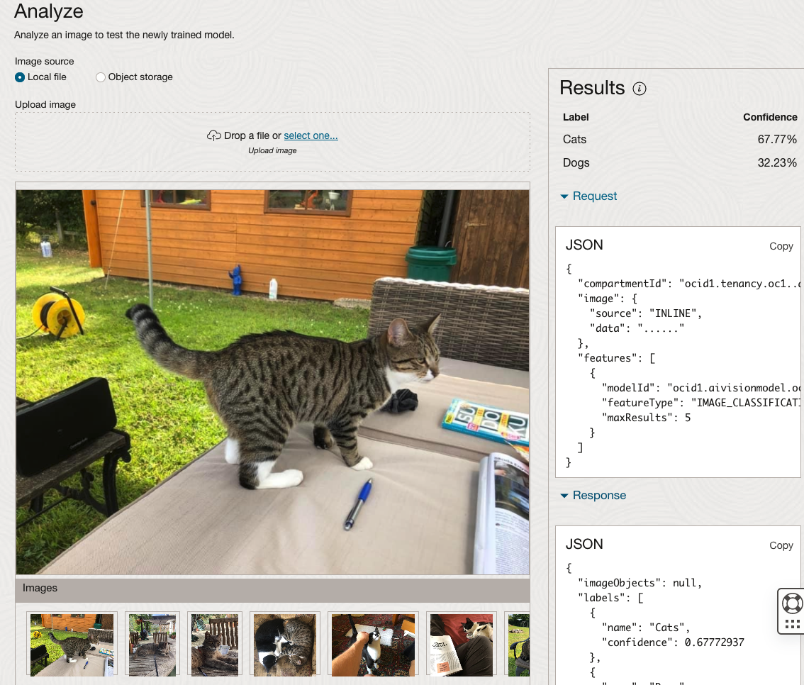
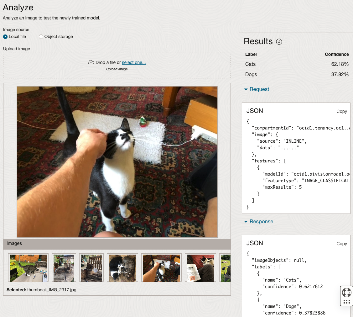
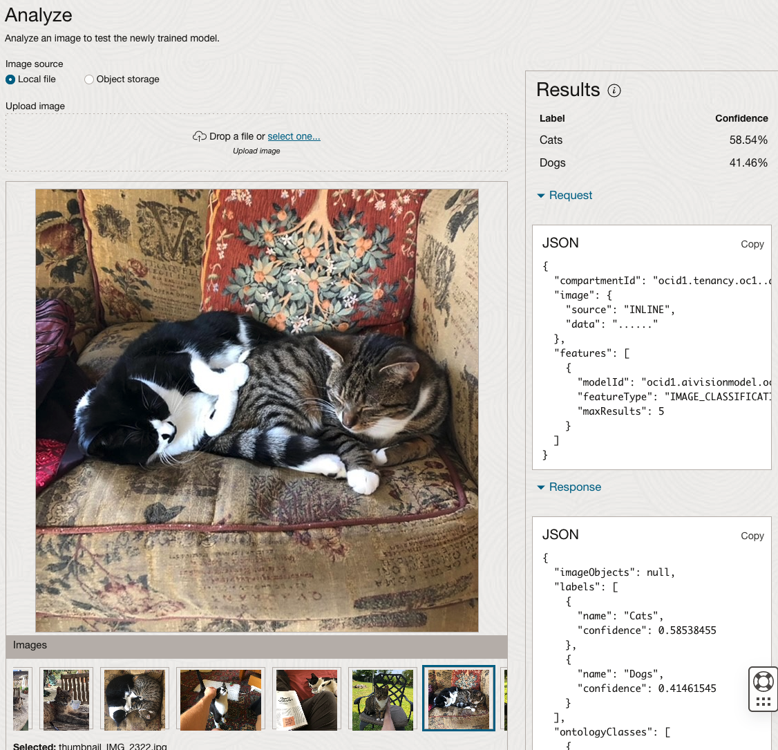
The bottom half of this page allows you to upload and evaluate images. The following images are example images of cats (do you know the owner) and the predictions and information about these are displayed on the screen. Have a look at the following to see which images scored better than others for identifying a Cat.
OCI:Vision – AI for image processing – the Basics
Every cloud service provides some form of AI offering. Some of these can range from very basic features right up to a mediocre level. Only a few are delivering advanced AI services in a useful way.
Oracle AI Services have been around for about a year now, and with all new products or cloud services, a little time is needed to let it develop from an MVP (minimum viable produce) to something that’s more mature, feature-rich, stable and reliable. Oracle’s OCI AI Services come with some pre-training models and to create your own custom models based on your own training datasets.
Oracle’s OCI AI Services include:
- Digital Assistant
- Language
- Speech
- Vision
- Document Understand
- Anomaly Detection
- Forecasting
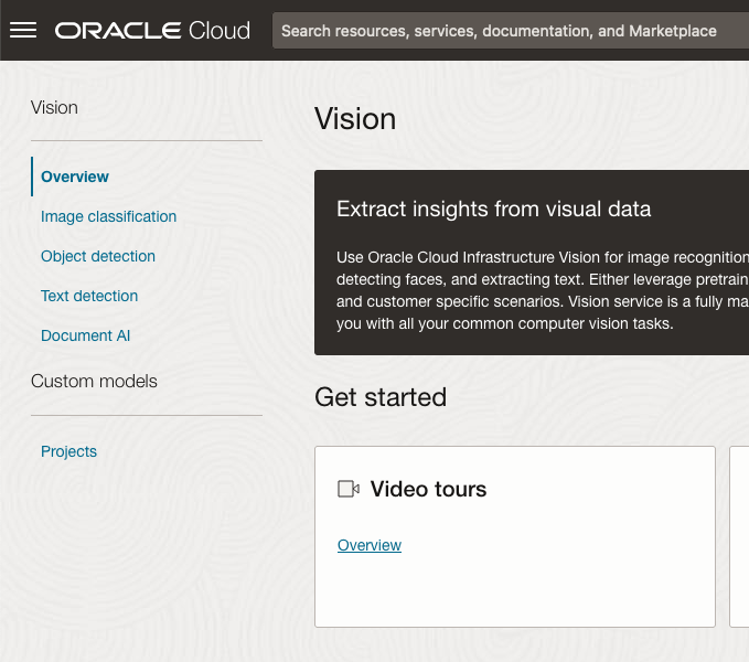
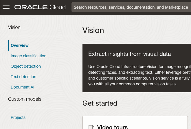
In this post, we’ll explore OCI Vision, and what the capabilities are available with their pre-trained models. To demonstrate this their online/webpage application will be used to demonstrate what it does and what it creates and identifies. You can access the Vision AI Services from the menu as shown in the following image.
From the main AI Vision webpage, we can see on the menu (on left-hand side of the page), we have three main Vision related options. These are Image Classification, Object Detection and Document AI. These are pre-trained models that perform slightly different tasks.
Let’s start with Image Classification and explore what is possible. Just Click on the link.
Note: The Document AI feature will be moving to its own cloud Service in 2024, so it will disappear from them many but will appear as a new service on the main Analytics & AI webpage (shown above).
The webpage for each Vision feature comes with a couple of images for you to examine to see how it works. But a better way to explore the capabilities of each feature is to use your own images or images you have downloaded. Here are examples.
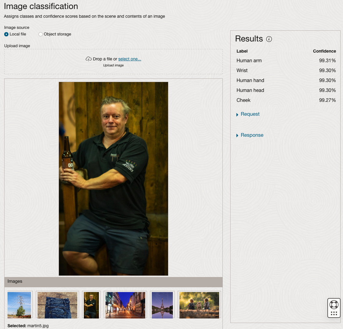
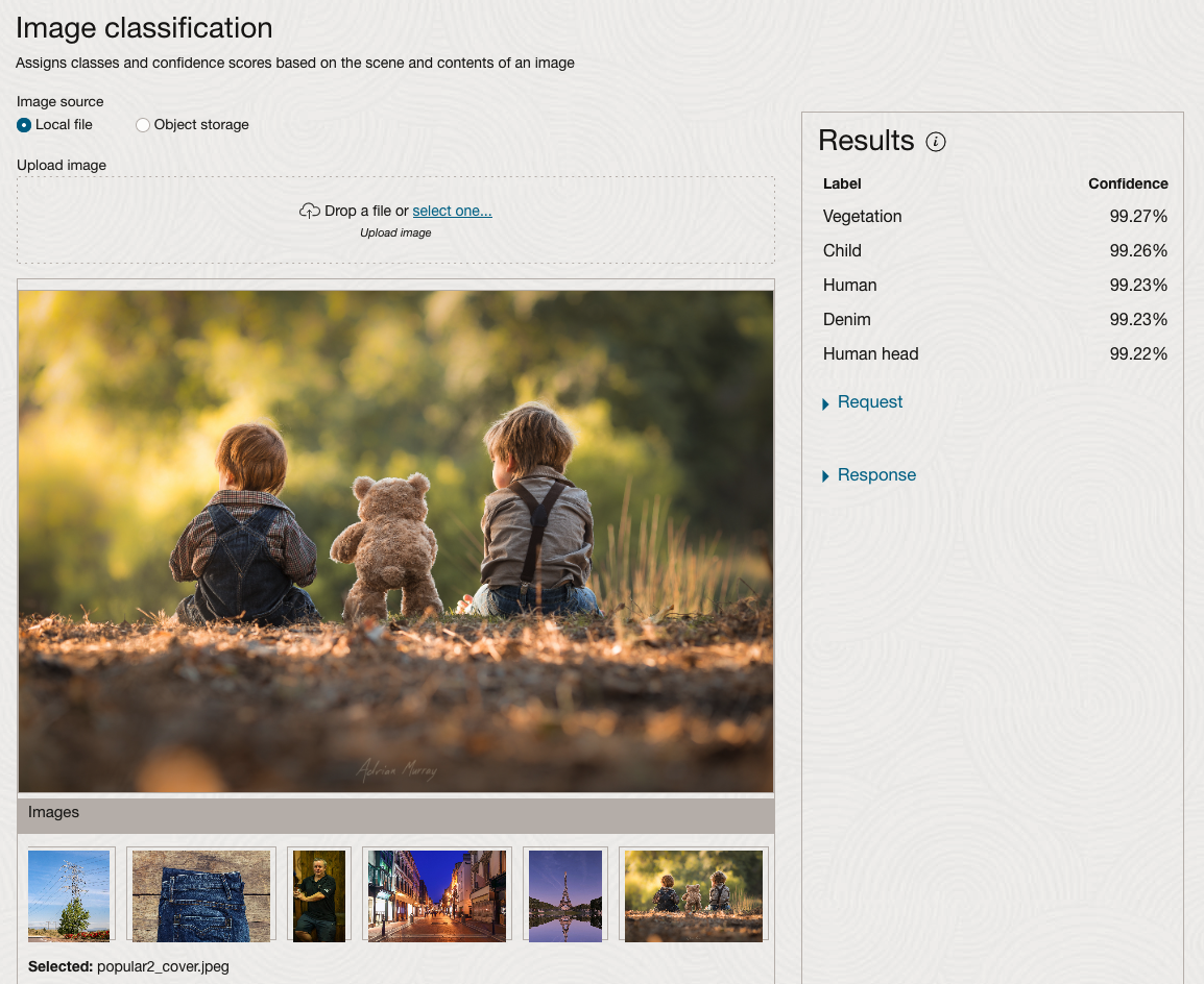
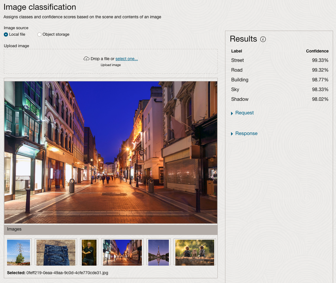
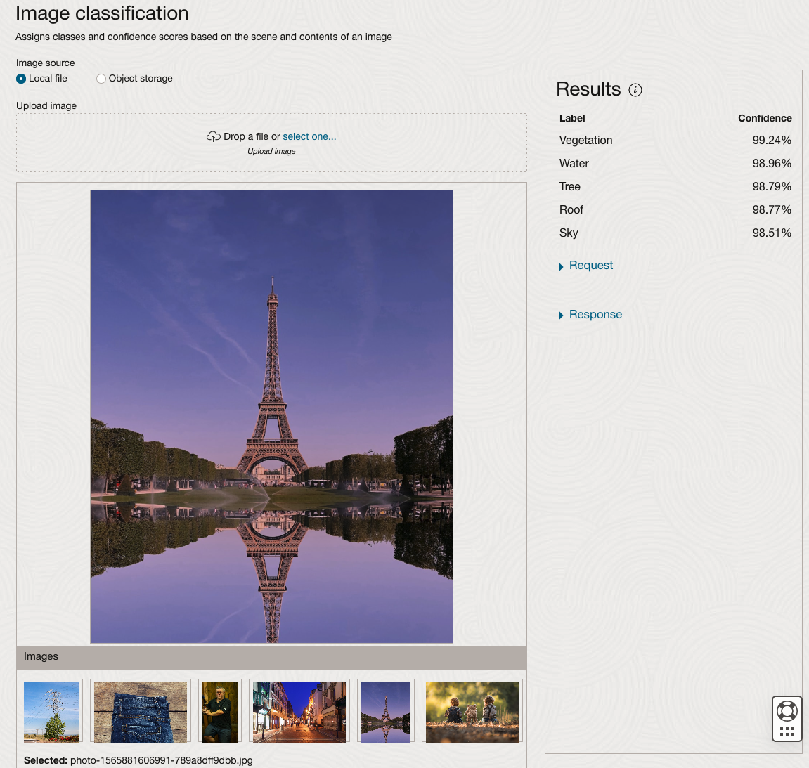
We can see the pre-trained model assigns classes and confidence for each image based on the main components it has identified in the image. For example with the Eiffel Tower image, the model has identified Water, Trees, Sky, Vegetation and Roof (of build). But it didn’t do so well with identifying the main object in the image as being a tower, or building of some form. Where with the streetscape image it was able to identify Street, Road, Building, Sky and Shadow.
Just under the Result section, we see two labels that can be expanded. One of these is the Response which contains JSON structure containing the labels, and confidences it has identified. This is what the pre-trained model returns and if you were to use Python to call this pre-trained model, it is this JSON object that you will get returned. You can then use the information contained in the JSON object to perform additional tasks for the image.
As you can see the webpage for OCI Vision and other AI services gives you a very simple introduction to what is possible, but it over simplifies the task and a lot of work is needed outside of this page to make the use of these pre-trained models useful.
Moving onto the Object Detection feature (left-hand menu) and using the pre-trained model on the same images, we get slightly different results.
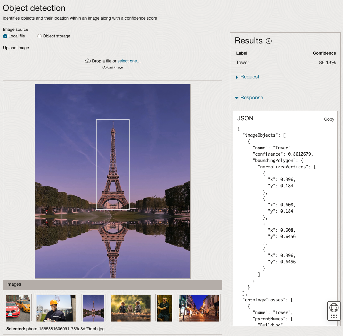
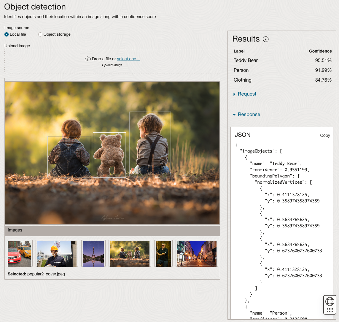
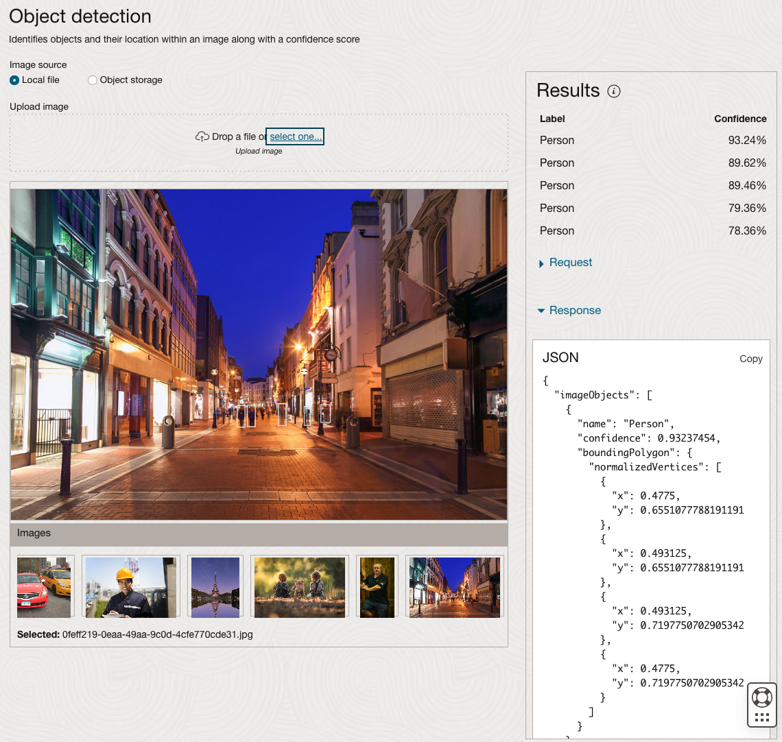
The object detection pre-trained model works differently as it can identify different things in the image. For example, with the Eiffel Tower image, it identifies a Tower in the image. In a similar way to the previous example, the model returns a JSON object with the label and also provides the coordinates for a bounding box for the objects detected. In the street scape image, it has identified five people. You’ll probably identify many more but the model identified five. Have a look at the other images and see what it has identified for each.
As I mentioned above, using these pre-trained models are kind of interesting, but are of limited use and do not really demonstrate the full capabilities of what is possible. Look out of additional post which will demonstrate this and steps needed to create and use your own custom model.
EU AI Act adopts OECD Definition of AI
Over the recent months, the EU AI Act has been making progress through the various hoop in the EU. Various committees and working groups have examined different parts of the AI Act and how it will impact the wider population. Their recommendations have been added to the EU Act and it has now progressed to the next stage for ratification in the EU Parliament which should happen in a few months time.
There are lots of terms within the EU AI Act which needed defining, with the most crucial one being the definition of AI, and this definition underpins the entire act, and all the other definitions of terms throughout the EU AI Act. Back in March of this year, the various political groups working on the EU AI Act reached an agreement on the definition of AI (Artificial Intelligence). The EI AI Act adopts, or is based on, the OECD definition of AI.
“Artificial intelligence system’ (AI system) means a machine-based system that is designed to operate with varying levels of autonomy and that can, for explicit or implicit objectives, generate output such as predictions, recommendations, or decisions influencing physical or virtual environments”

The working groups wanted the AI definition to be closely aligned with the work of international organisations working on artificial intelligence to ensure legal certainty, harmonisation and wide acceptance. The wording includes reference to predictions includes content, this is to ensure generative AI models like ChatGPT are included in the regulation.
Other definitions included are, significant risk, biometric authentication and identification.
“‘Significant risk’ means a risk that is significant in terms of its severity, intensity, probability of occurrence, duration of its effects, and its ability to affect an individual, a plurality of persons or to affect a particular group of persons,” the document specifies.
Remote biometric verification systems were defined as AI systems used to verify the identity of persons by comparing their biometric data against a reference database with their prior consent. That is distinguished by an authentication system, where the persons themselves ask to be authenticated.
On biometric categorisation, a practice recently added to the list of prohibited use cases, a reference was added to inferring personal characteristics and attributes like gender or health.
Machine Learning App Migration to Oracle Cloud VM
Over the past few years, I’ve been developing a Stock Market prediction algorithm and made some critical refinements to it earlier this year. As with all analytics, data science, machine learning and AI projects, testing is vital to ensure its performance, accuracy and sustainability. Taking such a project out of a lab environment and putting it into a production setting introduces all sorts of different challenges. Some of these challenges include being able to self-manage its own process, logging, traceability, error and event management, etc. Automation is key and implementing all of these extra requirements tasks way more code and time than developing the actual algorithm. Typically, the machine learning and algorithms code only accounts for less than five percent of the actual code, and in some cases, it can be less than one percent!
I’ve come to the stage of deploying my App to a production-type environment, as I’ve been running it from my laptop and then a desktop for over a year now. It’s now 100% self-managing so it’s time to deploy. The environment I’ve chosen is using one of the Virtual Machines (VM) available on the Oracle Free Tier. This means it won’t cost me a cent (dollar or more) to run my App 24×7.
My App has three different components which use a core underlying machine learning predictions engine. Each is focused on a different set of stock markets. These marks operate in the different timezone of US markets, European Markets and Asian Markets. Each will run on a slightly different schedule than the rest.
The steps outlined below take you through what I had to do to get my App up and running the VM (Oracle Free Tier). It took about 20 minutes to complete everything
The first thing you need to do is create a ssh key file. There are a number of ways of doing this and the following is an example.
ssh-keygen -t rsa -N "" -b 2048 -C "myOracleCloudkey" -f myOracleCloudkey
This key file will be used during the creation of the VM and for logging into the VM.
Log into your Oracle Cloud account and you’ll find the Create Instances Compute i.e. create a virtual machine/

Complete the Create Instance form and upload the ssh file you created earlier. Then click the Create button. This assumes you have networking already created.

It will take a minute or two for the VM to be created and you can monitor the progress.
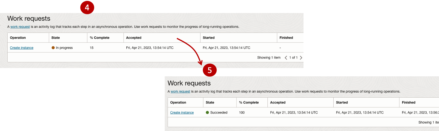
After it has been created you need to click on the start button to start the VM.
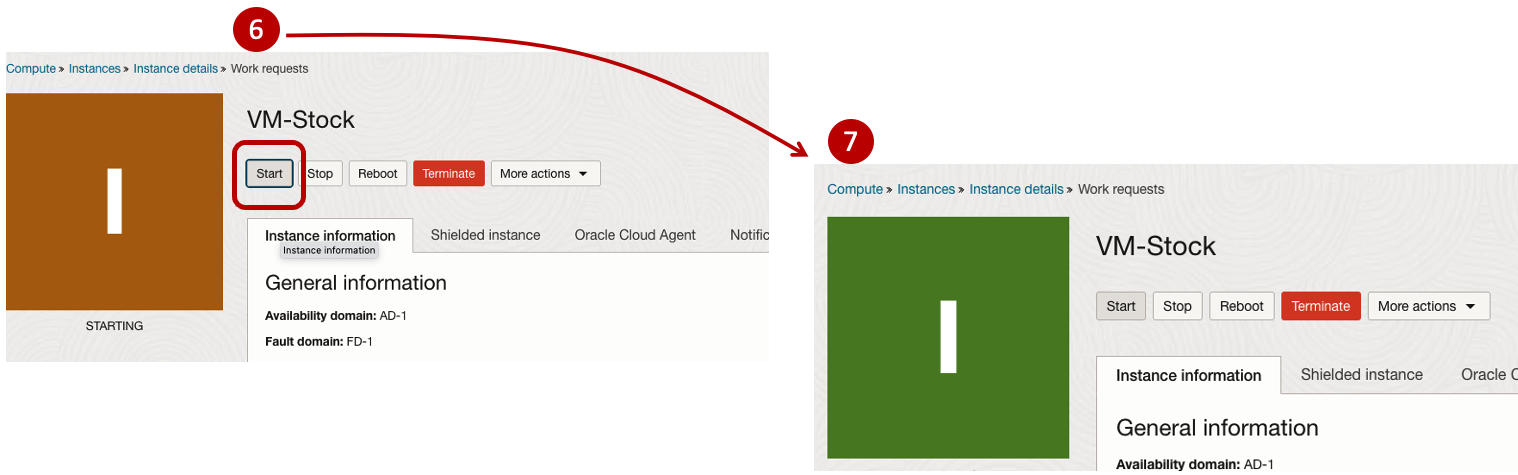
After it has started you can now log into the VM from a terminal window, using the public IP address
ssh -i myOracleCloudKey opc@xxx.xxx.xxx.xxxAfter you’ve logged into the VM it’s a good idea to run an update.
[opc@vm-stocks ~]$ sudo yum -y update
Last metadata expiration check: 0:13:53 ago on Fri 21 Apr 2023 14:39:59 GMT.
Dependencies resolved.
========================================================================================================================
 Package                         Arch       Version                                          Repository            Size
========================================================================================================================
Installing:
 kernel-uek                      aarch64    5.15.0-100.96.32.el8uek                          ol8_UEKR7            1.4 M
 kernel-uek-core                 aarch64    5.15.0-100.96.32.el8uek                          ol8_UEKR7             47 M
 kernel-uek-devel                aarch64    5.15.0-100.96.32.el8uek                          ol8_UEKR7             19 M
 kernel-uek-modules              aarch64    5.15.0-100.96.32.el8uek                          ol8_UEKR7             59 M
Upgrading:
 NetworkManager                  aarch64    1:1.40.0-6.0.1.el8_7                             ol8_baseos_latest    2.1 M
 NetworkManager-config-server    noarch     1:1.40.0-6.0.1.el8_7                             ol8_baseos_latest    141 k
 NetworkManager-libnm            aarch64    1:1.40.0-6.0.1.el8_7                             ol8_baseos_latest    1.9 M
 NetworkManager-team             aarch64    1:1.40.0-6.0.1.el8_7                             ol8_baseos_latest    156 k
 NetworkManager-tui              aarch64    1:1.40.0-6.0.1.el8_7                             ol8_baseos_latest    339 k
...
...
The VM is now ready to setup and install my App. The first step is to install Python, as all my code is written in Python.
[opc@vm-stocks ~]$ sudo yum install -y python39
Last metadata expiration check: 0:20:35 ago on Fri 21 Apr 2023 14:39:59 GMT.
Dependencies resolved.
========================================================================================================================
 Package                         Architecture  Version                                        Repository           Size
========================================================================================================================
Installing:
 python39                        aarch64       3.9.13-2.module+el8.7.0+20879+a85b87b0         ol8_appstream        33 k
Installing dependencies:
 python39-libs                   aarch64       3.9.13-2.module+el8.7.0+20879+a85b87b0         ol8_appstream       8.1 M
 python39-pip-wheel              noarch        20.2.4-7.module+el8.6.0+20625+ee813db2         ol8_appstream       1.1 M
 python39-setuptools-wheel       noarch        50.3.2-4.module+el8.5.0+20364+c7fe1181         ol8_appstream       497 k
Installing weak dependencies:
 python39-pip                    noarch        20.2.4-7.module+el8.6.0+20625+ee813db2         ol8_appstream       1.9 M
 python39-setuptools             noarch        50.3.2-4.module+el8.5.0+20364+c7fe1181         ol8_appstream       871 k
Enabling module streams:
 python39                                      3.9

Transaction Summary
========================================================================================================================
Install  6 Packages

Total download size: 12 M
Installed size: 47 M
Downloading Packages:
(1/6): python39-pip-20.2.4-7.module+el8.6.0+20625+ee813db2.noarch.rpm                    23 MB/s | 1.9 MB     00:00
(2/6): python39-pip-wheel-20.2.4-7.module+el8.6.0+20625+ee813db2.noarch.rpm             5.5 MB/s | 1.1 MB     00:00
...
...
Next copy the code to the VM, setup the environment variables and create any necessary directories required for logging. The final part of this is to download the connection Wallett for the Database. I’m using the Python library oracledb, as this requires no additional setup.
Then install all the necessary Python libraries used in the code, for example, pandas, matplotlib, tabulate, seaborn, telegram, etc (this is just a subset of what I needed). For example here is the command to install pandas.
pip3.9 install pandasAfter all of that, it’s time to test the setup to make sure everything runs correctly.
The final step is to schedule the App/Code to run. Before setting the schedule just do a quick test to see what timezone the VM is running with. Run the date command and you can see what it is. In my case, the VM is running GMT which based on the current time locally, the VM was showing to be one hour off. Allowing for this adjustment and for day-light saving time, the time +/- markets openings can be set. The following example illustrates setting up crontab to run the App, Monday-Friday, between 13:00-22:00 and at 5-minute intervals. Open crontab and edit the schedule and command. The following is an example
> contab -e

*/5 13-22 * * 1-5 python3.9 /home/opc/Stocks.py >Stocks.txt
For some stock market trading apps, you might want it to run more frequently (than every 5 minutes) or less frequently depending on your strategy.
After scheduling the components for each of the Geographic Stock Market areas, the instant messaging of trades started to appear within a couple of minutes. After a little monitoring and validation checking, it was clear everything was running as expected. It was time to sit back and relax and see how this adventure unfolds.
For anyone interested, the App does automated trading with different brokers across the markets, while logging all events and trades to an Oracle Autonomous Database (Free Tier = no cost), and sends instant messages to me notifying me of the automated trades. All I have to do is Nothing, yes Nothing, only to monitor the trade notifications. I mentioned earlier the importance of testing, and with back-testing of the recent changes/improvements (as of the date of post), the App has given a minimum of 84% annual return each year for the past 15 years. Most years the return has been a lot more!
Preparing images for #DeepLearning by removing background
There are a number of methods available for preparing images for input to a variety of purposes. For example, for input to deep learning, other image processing models/applications/systems, etc. But sometimes you just need a quick tool to perform a certain task. An example of this is I regularly have to edit images to extract just a certain part of it, or to filter out all the background colors and/or objects etc. There are a a variety of tools available to help you with this kind of task. For me, I’m a Mac user, so I use the instant alpha feature available in some of the Mac products. But what if you are not a Mac user, what can you use.
I’ve recently come across a very useful Python library that takes all or most of the hard work out of doing such tasks, and has proved to be extremely useful for some demos and projects I’ve been working on. The Python library I’m using is remgb (Remove Background). It isn’t perfect, but it does a pretty good job and only in a small number of modified images, did I need to do some additional processing.
Let’s get started with setting things up to use remgb. I did encounter some minor issues installing it, and I’ve give the workarounds below, just in case you encounter the same.
pip3 install remgbThis will install lots of required libraries and will check for compatibility with what you have installed. The first time I ran the install it generated some errors. It also suggested I update my version of pip, which I did, then uninstalled the remgb library and installed again. No errors this time.
When I ran the code below, I got some errors about accessing a document on google drive or it had reached the maximum number of views/downloads. The file it is trying to access is an onix model. If you click on the link, you can download the file. Create a directory called .u2net (in your home directory) and put the onix file into it. Make sure the directory is readable. After doing that everything runs smoothly for me.
The code I’ve given below is typical of what I’ve been doing on some projects. I have a folder with lots of images where I want to remove the background and only keep the key foreground object. Then save the modified images to another directory. It is these image that can be used in products like Amazon Rekognition, Oracle AI Services, and lots of other similar offerings.
from rembg import remove
from PIL import Image
import os
from colorama import Fore, Back, Style
sourceDir = '/Users/brendan.tierney/Dropbox/4-Datasets/F1-Drivers/'
destDir = '/Users/brendan.tierney/Dropbox/4-Datasets/F1-Drivers-NewImages/'
print('Searching = ', sourceDir)
files = os.listdir(sourceDir)
for file in files:
try:
inputFile = sourceDir + file
outputFile = destDir + file
with open(inputFile, 'rb') as i:
print(Fore.BLACK + '..reading file : ', file)
input = i.read()
print(Fore.CYAN + '...removing background...')
output = remove(input)
try:
with open(outputFile, 'wb') as o:
print(Fore.BLUE + '.....writing file : ', outputFile)
o.write(output)
except:
print(Fore.RED + 'Error writing file :', outputFile)
except:
print(Fore.RED + 'Error processing file :', file)
print(Fore.BLACK + '---')
print(Fore.BLACK + 'Finished processing all files')
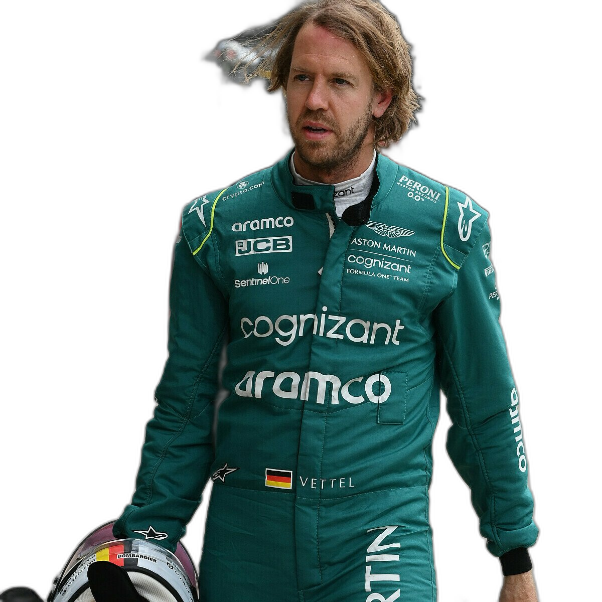
print(Fore.BLACK + '---')For this demonstration I’ve used images of the F1 drivers for 2022. I had collected five images of each driver with different backgrounds including, crowds, pit-lane, giving media interviews, indoor and outdoor images.
Generally the results were very good. Here are some results with the before and after.


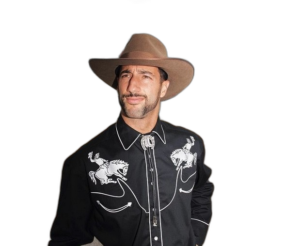


As you can see from these image there are some where a shadow remains and the library wasn’t able to remove it. The following images gives some additional examples of this. The first is with Bottas and his car, where the car wasn’t removed. The second driver is Vettel where the library captures his long hair and keeps it in the filtered image.


Postgres on Docker
Prostgres is one of the most popular databases out there, being used in Universities, open source projects and also widely used in the corporate marketplace. I’ve written a previous post on running Oracle Database on Docker. This post is similar, as it will show you the few simple steps to have a persistent Postgres Database running on Docker.
The first step is go to Docker Hub and locate the page for Postgres. You should see something like the following. Click through to the Postgres page.

There are lots and lots of possible Postgres images to download and use. The simplest option is to download the latest image using the following command in a command/terminal window. Make sure Docker is running on your machine before running this command.
docker pull postgresAlthough, if you needed to install a previous release, you can do that.

After the docker image has been downloaded, you can now import into Docker and create a container.
docker run --name postgres -p 5432:5432 -e POSTGRES_USER=postgres -e POSTGRES_PASSWORD=pgPassword -e POSTGRES_DB=postgres -d postgresImportant: I’m using Docker on a Mac. If you are using Windows, the format of the parameter list is slightly different. For example, remove the = symbol after POSTGRES_DB
If you now check with Docker you’ll see Postgres is now running on post 5432.

Next you will need pgAdmin to connect to the Postgres Database and start working with it. You can download and install it, or run another Docker container with pgAdmin running in it.
First, let’s have a look at installing pgAdmin. Download the image and run, accepting the initial requirements. Just let it run and finish installing.


When pgAdmin starts it looks for you to enter a password. This can be anything really, but one that you want to remember. For example, I set mine to pgPassword.
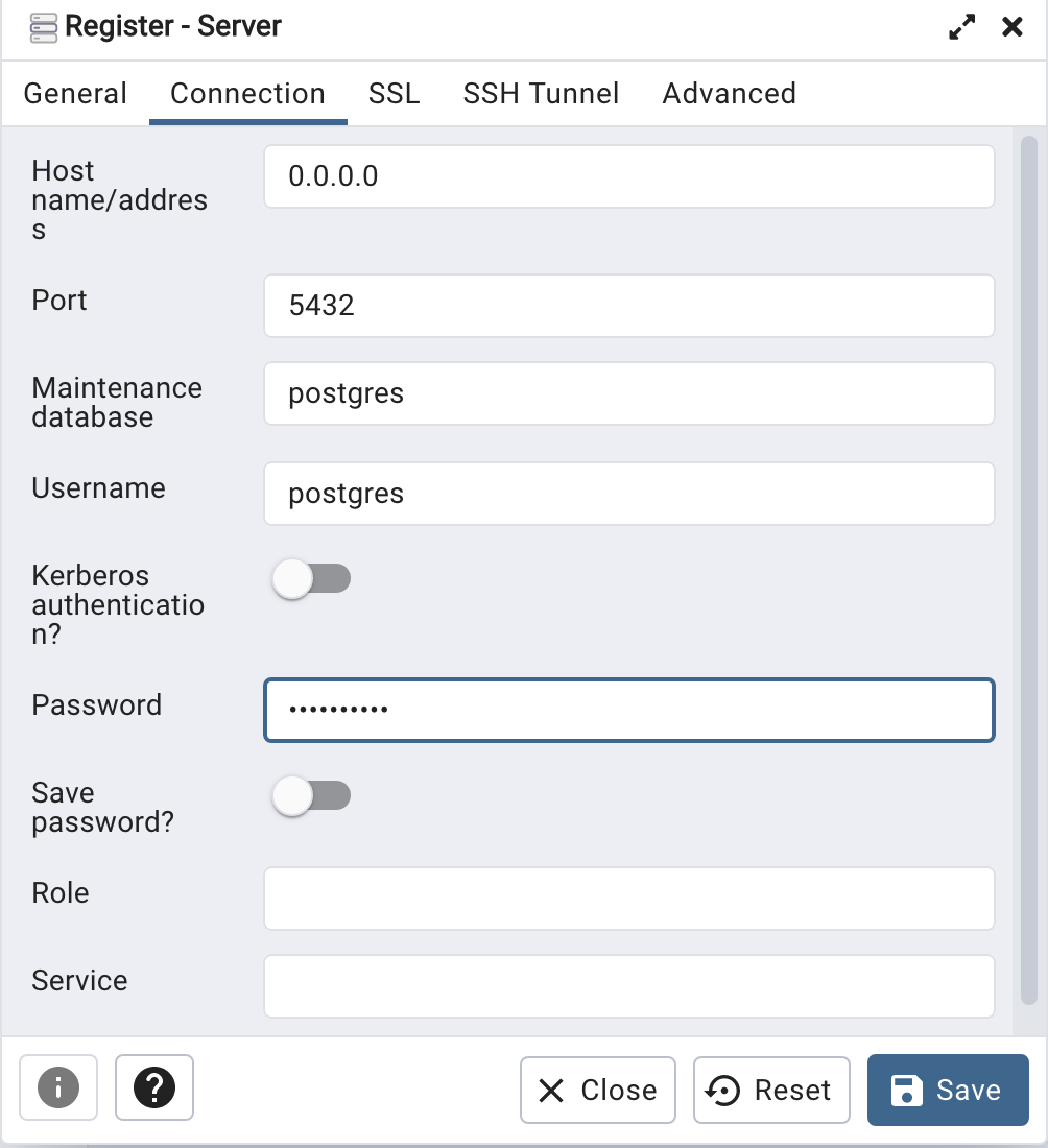
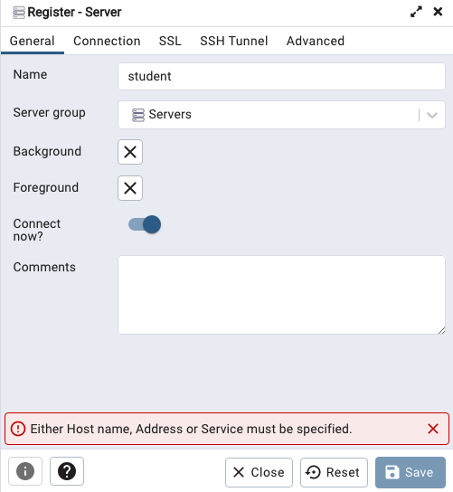
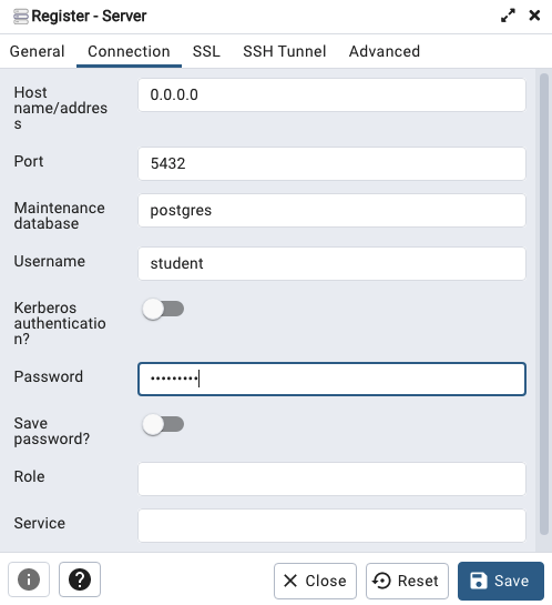
Then create (or Register) a connection to your Postgres Database. Enter the details you used when creating the docker image including username=postgres, password=pgPassword and IP address=0.0.0.0.
The IP address on your machine might be a little different, and to check what it is, run the following
docker ps -a


When your (above) connection works, the next step is to create another schema/user in the database. The reason we need to do this is because the user we connected to above (postgres) is an admin user. This user/schema should never be used for database development work.
Let’s setup a user we can use for our development work called ‘student’. To do this, right click on the ‘postgres’ user connection and open the query tool.
Then run the following.

After these two commands have been run successfully we can now create a connection to the postgres database, open the query tool and you’re now all set to write some SQL.


You must be logged in to post a comment.