
Uncategorized
GoLang: Inserting records into Oracle Database using goracle
In this blog post I’ll give some examples of how to process data for inserting into a table in an Oracle Database. I’ve had some previous blog posts on how to setup and connecting to an Oracle Database, and another on retrieving data from an Oracle Database and the importance of setting the Array Fetch Size.
When manipulating data the statements can be grouped (generally) into creating new data and updating existing data.
When working with this kind of processing we need to avoid the creation of the statements as a concatenation of strings. This opens the possibility of SQL injection, plus we are not allowing the optimizer in the database to do it’s thing. Prepared statements allows for the reuse of execution plans and this in turn can speed up our data processing and applications.
In a previous blog post I gave a simple example of a prepared statement for querying data and then using it to pass in different values as a parameter to this statement.
dbQuery, err := db.Prepare("select cust_first_name, cust_last_name, cust_city from sh.customers where cust_gender = :1")
if err != nil {
    fmt.Println(err)
    return
}
defer dbQuery.Close()

rows, err := dbQuery.Query('M')
if err != nil {
    fmt.Println(".....Error processing query")
    fmt.Println(err)
    return
}
defer rows.Close()

var CustFname, CustSname,CustCity string
for rows.Next() {
    rows.Scan(&CustFname, &CustSname, &CustCity)
    fmt.Println(CustFname, CustSname, CustCity)
}
For prepared statements for inserting data we can follow a similar structure. In the following example a table call LAST_CONTACT is used. This table has columns:
- CUST_ID
- CON_METHOD
- CON_MESSAGE
_, err := db.Exec("insert into LAST_CONTACT(cust_id, con_method, con_message) VALUES(:1, :2, :3)", 1, "Phone", "First contact with customer")
if err != nil {
    fmt.Println(".....Error Inserting data")
    fmt.Println(err)
    return
}
an alternative is the following and allows us to get some additional information about what was done and the result from it. In this example we can get the number records processed.
stmt, err := db.Prepare("insert into LAST_CONTACT(cust_id, con_method, con_message) VALUES(:1, :2, :3)")
if err != nil {
    fmt.Println(err)
    return
}

res, err := dbQuery.Query(1, "Phone", "First contact with customer")
if err != nil {
    fmt.Println(".....Error Inserting data")
    fmt.Println(err)
    return
}

rowCnt := res.RowsAffected()
fmt.Println(rowCnt, " rows inserted.")
A similar approach can be taken for updating and deleting records
Managing Transactions
With transaction, a number of statements needs to be processed as a unit. For example, in double entry book keeping we have two inserts. One Credit insert and one debit insert. To do this we can define the start of a transaction using db.Begin() and the end of the transaction with a Commit(). Here is an example were we insert two contact details.
// start the transaction
transx, err := db.Begin()
if err != nil {
    fmt.Println(err)
    return
}

// Insert first record
_, err := db.Exec("insert into LAST_CONTACT(cust_id, con_method, con_message) VALUES(:1, :2, :3)", 1, "Email", "First Email with customer")
if err != nil {
    fmt.Println(".....Error Inserting data - first statement")
    fmt.Println(err)
    return
}
// Insert second record
_, err := db.Exec("insert into LAST_CONTACT(cust_id, con_method, con_message) VALUES(:1, :2, :3)", 1, "In-Person", "First In-Person with customer")
if err != nil {
    fmt.Println(".....Error Inserting data - second statement")
    fmt.Println(err)
    return
}

// complete the transaction
err = transx.Commit()
if err != nil {
    fmt.Println(".....Error Committing Transaction")
    fmt.Println(err)
    return
}
Embedding Transformation Data Pipeline into ML Model using Oracle Data Mining
I’ve written several blog posts about how to use the DBMS_DATA_MINING.TRANSFORM function to create various data transformations and how to apply these to your data. All of these steps can be simple enough to following and re-run in a lab environment. But the real value with data science and machine learning comes when you deploy the models into production and have the ML models scoring data as it is being produced, and your applications acting upon these predictions immediately, and not some hours or days later when the data finally arrives in the lab environment.
It would be useful to be able to bundle all the transformations into the same process the create the model. The transformations and model become one, together. If this is possible, then that greatly simplifies how the ML model can be deployed into production. It then becomes a simple function or REST call. We need to keep this simple (KISS).
Using the examples from my previous blog posts performing various data transformations, the following example shows how you can bundle these up into one defined set of transformations and then embed these transformations as part of the ML model. To do this we need to define a list of transformations. We can do this using:
xform_list IN TRANSFORM_LIST DEFAULT NULL
Where TRANSFORM_LIST has the following structure:
TRANFORM_REC IS RECORD (
     attribute_name       VARCHAR2(4000),
     attribute_subname    VARCHAR2(4000),
     expression           EXPRESSION_REC,
     reverse_expression   EXPRESSION_REC,
     attribute_spec       VARCHAR2(4000));
You can use the DBMS_DATA_MINING.SET_TRANSFORM function to defined the transformations. The following example illustrates the transformation of converting the BOOKKEEPING_APPLICATION attribute from a number data type to a character data type.
DECLARE
   transform_stack   dbms_data_mining_transform.TRANSFORM_LIST;
BEGIN
   dbms_data_mining_transform.SET_TRANSFORM(transform_stack,
                                  'BOOKKEEPING_APPLICATION',
                                  NULL,
                                  'to_char(BOOKKEEPING_APPLICATION)',
                                  'to_number(BOOKKEEPING_APPLICATION)',
                                  NULL);
END;
Alternatively you can use the SET_EXPRESSION function and then create the transformation using it.
You can Stack the transforms together. Using the above example you could express a number of transformations and have these stored in the TRANSFORM_STACK variable. You can then pass this variable into your CREATE_MODEL procedure and have these transformations embedded in your ML model.
DECLARE
   transform_stack   dbms_data_mining_transform.TRANSFORM_LIST;
BEGIN
   -- Define the transformation list
   dbms_data_mining_transform.SET_TRANSFORM(transform_stack,
                                  'BOOKKEEPING_APPLICATION',
                                  NULL,
                                  'to_char(BOOKKEEPING_APPLICATION)',
                                  'to_number(BOOKKEEPING_APPLICATION)',
                                  NULL);

   -- Create the data mining model
   DBMS_DATA_MINING.CREATE_MODEL(
      model_name           => 'DEMO_TRANSFORM_MODEL',
      mining_function      => dbms_data_mining.classification,
      data_table_name      => 'MINING_DATA_BUILD_V',
      case_id_column_name  => 'cust_id',
      target_column_name   => 'affinity_card',
      settings_table_name  => 'demo_class_dt_settings',
      xform_list           => transform_stack);
END;
My previous blog posts showed how to create various types of transformations. These transformations were then used to create a view of the data set that included these transformations. To embed these transformations in the ML Model we need to use the STACK function. The following examples illustrate the stacking of the transformations created in the previous blog posts. These transformations are added (or stacked) to a transformation list and then added to the CREATE_MODEL function, embedding these transformations in the model.
DECLARE
   transform_stack   dbms_data_mining_transform.TRANSFORM_LIST;
BEGIN
   -- Stack the missing numeric transformations
   dbms_data_mining_transform.STACK_MISS_NUM (
          miss_table_name   => 'TRANSFORM_MISSING_NUMERIC',
          xform_list        => transform_stack);

   -- Stack the missing categorical transformations
   dbms_data_mining_transform.STACK_MISS_CAT (
          miss_table_name   => 'TRANSFORM_MISSING_CATEGORICAL',
          xform_list        => transform_stack);

   -- Stack the outlier treatment for AGE
   dbms_data_mining_transform.STACK_CLIP (
          clip_table_name   => 'TRANSFORM_OUTLIER',
          xform_list        => transform_stack);

   -- Stack the normalization transformation
   dbms_data_mining_transform.STACK_NORM_LIN (
          norm_table_name   => 'MINING_DATA_NORMALIZE',
          xform_list        => transform_stack);

   -- Create the data mining model
   DBMS_DATA_MINING.CREATE_MODEL(
      model_name           => 'DEMO_STACKED_MODEL',
      mining_function      => dbms_data_mining.classification,
      data_table_name      => 'MINING_DATA_BUILD_V',
      case_id_column_name => 'cust_id',
      target_column_name   => 'affinity_card',
      settings_table_name => 'demo_class_dt_settings',
      xform_list           => transform_stack);
END;
To view the embedded transformations in your data mining model you can use the GET_MODEL_TRANSFORMATIONS function.
SELECT TO_CHAR(expression)
FROM TABLE (dbms_data_mining.GET_MODEL_TRANSFORMATIONS('DEMO_STACKED_MODEL'));
TO_CHAR(EXPRESSION)
--------------------------------------------------------------------------------
(CASE  WHEN (NVL("AGE",38.892)<18) THEN 18 WHEN (NVL("AGE",38.892)>70) THEN 70 E
LSE NVL("AGE",38.892) END -18)/52

NVL("BOOKKEEPING_APPLICATION",.880667)
NVL("BULK_PACK_DISKETTES",.628)
NVL("FLAT_PANEL_MONITOR",.582)
NVL("HOME_THEATER_PACKAGE",.575333)
NVL("OS_DOC_SET_KANJI",.002)
NVL("PRINTER_SUPPLIES",1)
(CASE  WHEN (NVL("YRS_RESIDENCE",4.08867)<1) THEN 1 WHEN (NVL("YRS_RESIDENCE",4.
08867)>8) THEN 8 ELSE NVL("YRS_RESIDENCE",4.08867) END -1)/7

NVL("Y_BOX_GAMES",.286667)
NVL("COUNTRY_NAME",'United States of America')
NVL("CUST_GENDER",'M')
NVL("CUST_INCOME_LEVEL",'J: 190,000 - 249,999')
NVL("CUST_MARITAL_STATUS",'Married')
NVL("EDUCATION",'HS-grad')
NVL("HOUSEHOLD_SIZE",'3')
NVL("OCCUPATION",'Exec.')
Transforming Outliers in Oracle Data Mining
In previous posts I’ve shown how to use the DBMS_DATA_MINING.TRANSFORM function to transform data is various ways including, normalization and missing data. In this post I’ll build upon these to show how to outliers can be handled.
The following example will show you how you can transform data to identify outliers and transform them. In the example, Winsorsizing transformation is performed where the outlier values are replaced by the nearest value that is not an outlier.
The transformation process takes place in three stages. For the first stage a table is created to contain the outlier transformation data. The second stage calculates the outlier transformation data and store these in the table created in stage 1. One of the parameters to the outlier procedure requires you to list the attributes you do not the transformation procedure applied to (this is instead of listing the attributes you do want it applied to). The third stage is to create a view (MINING_DATA_V_2) that contains the data set with the outlier transformation rules applied. The input data set to this stage can be the output from a previous transformation process (e.g. DATA_MINING_V).
BEGIN
   -- Clean-up : Drop the previously created tables
   BEGIN
      execute immediate 'drop table TRANSFORM_OUTLIER';
   EXCEPTION
      WHEN others THEN
         null;
   END;

   -- Stage 1 : Create the table for the transformations
   -- Perform outlier treatment for: AGE and YRS_RESIDENCE
   --
   DBMS_DATA_MINING_TRANSFORM.CREATE_CLIP (
      clip_table_name => 'TRANSFORM_OUTLIER');

   -- Stage 2 : Transform the categorical attributes
   --   Exclude the number attributes you do not want transformed
   DBMS_DATA_MINING_TRANSFORM.INSERT_CLIP_WINSOR_TAIL (
      clip_table_name => 'TRANSFORM_OUTLIER',
      data_table_name => 'MINING_DATA_V',
      tail_frac       => 0.025,
      exclude_list    => DBMS_DATA_MINING_TRANSFORM.COLUMN_LIST (
                          'affinity_card',
                          'bookkeeping_application',
                          'bulk_pack_diskettes',
                          'cust_id',
                          'flat_panel_monitor',
                          'home_theater_package',
                          'os_doc_set_kanji',
                          'printer_supplies',
                          'y_box_games'));

   -- Stage 3 : Create the view with the transformed data
   DBMS_DATA_MINING_TRANSFORM.XFORM_CLIP(
      clip_table_name => 'TRANSFORM_OUTLIER',
      data_table_name => 'MINING_DATA_V',
      xform_view_name => 'MINING_DATA_V_2');
END;
The view MINING_DATA_V_2 will now contain the data from the original data set transformed to process missing data for numeric and categorical data (from previous blog post), and also has outlier treatment for the AGE attribute.
Examples of Machine Learning with Facial Recognition
In a previous blog post I gave some examples of how facial images recognition and videos are being used in our daily lives. In this post I want to extend this with some additional examples. There are ethical issues around this and in some of these examples their usage has stopped. What is also interesting is the reaction on various social media channels about this. People don’t like it and and happen that some of these have stopped.
But how widespread is this technology? Based on these known examples, and this list is by no means anywhere near complete, but gives an indication of the degree of it’s deployment and how widespread it is.
Dubai is using facial recognition to measure customer satisfaction at four of the Roads and Transport Authority Customer Happiness Centers. They analyze the faces of their customers and rank their level of happiness. They can use this to generate alerts when the happiness levels falls below certain levels.

Various department stores are using facial recognition throughout the stores and at checkout. These are being used to delivery personalized adverts to users on either in-store screen or on personalized screens on the shopping trolley. And can be used to verify a person’s age if they are buying alcohol or other products. Tesco’s have previously used face-scanning cameras at tills in petrol stations to target advertisements at customers depending on their age and approximate age.
Some retail stores are using ML to monitor you, monitor what items you pick up and what you pay for at the checkout, identifying any differences and what steps to take next.
In a slight variation of facial recognition, some stores are using similar technology to monitor stock levels, monitor how people interact with different products (e.g pick up one product and then relate it with a similar product), and optimized location of products. Walmart has been a learner in the are of AI and Machine Learning in the retail section for some time now.
The New York Metropolitan Transport Authority has been using facial capture and recognition at several site across the city. Their proof of concept location was at the Robert F Kennedy Bridge. The company supplying the technology claimed 80% accuracy at predicting the person, through a widescreen while the car was traveling at low speed. These images can then be matched against government databases, such as driver license authorities, police databases and terrorist databases. The problem with this project was that it did not achieve one single positive match (within acceptable parameters) during the initial period of the project.

There are some reports that similar technology is being use on the New York Subway system in Time Square to help with identifying fare dodgers.
How about using facial recognition at boarding gates for your new flight instead of showing your passport or other official photo id. JetBlue and other airlines are now using this technology. Some airports have been using this for many many years.

San Francisco City government took steps in May 2019 to ban the use of facial recognition across all city functions. Other cities like Oakland and Sommerville in Massachusetts have implemented similar bans with other cities likely to follow. But it doesn’t ban the use by private companies.

What about using this technology to automatically monitor and manage staff. Manage staff, as in to decide who should be fired and who should be reallocated elsewhere. It is reported that Amazon is using facial and other recognition systems to monitor staff productivity in their warehouses.

A point I highlighted in my previous post was how are these systems/applications able to get enough images as training samples for their models. This is considering that most of the able systems/applications say they don’t keep any of the images they capture.
How many of us take pictures and post them on Facebook, Instagram, Snapchat, Twitter, etc. By doing this, you are making those images available to these companies to training their machine learning model. To do this they scrap the images for these sites and then have to manually label them with descriptive information. It is a combination of the image and descriptive information that is used by the machine learning algorithms to learn and build a model that suits their needs. See the MIT Technology Review article for more details and example on this topic.

There are also reports of some mobile phone apps that turn on your mobile phone camera. The apps will detect if the phone is possibly mounted on the dashboard of a car, and then takes pictures of the inside of the car and also pictures of where you are driving. Similar reports exists about many apps and voice activated devices.
So be careful what you post on social media or anywhere else online, and be careful of what apps you have on your mobile phone!
There is a general backlash to the use of this technology, and with more people becoming aware of what is happening, we need to more aware of what when and where this technology is being used.
Transforming Missing Data using Oracle Data Mining
In a previous post I showed how you can normalize data using the in-database machine learning feature using the DBMS_DATA_MINING.TRANSFORM function. This same function can be used to perform many more data transformations with standardized routines. When it comes to missing data, where you have some case records where the value for an attribute is missing you have a number of options open to you. The first is to evaluate the degree of missing values for the attribute for the data set as a whole. If it is very high, you may want to remove that attribute from the data set. But in scenarios when you have a small number or percentage of missing values you will want to find an appropriate or an approximate value. Such calculations can involve the use of calculating the mean or mode.
To build this up using DBMS_DATA_MINING.TRANSFORM function, we need to follow a simple three stage process. The first stage creates a table that will contain the details of the transformations. The second stage defines and runs the transformation function to calculate the replacement values and finally, the third stage, to create the necessary records in the table created in the previous stage. These final two stages need to be followed for both numerical and categorical attributes. For the final stage you can create a new view that contains the data from the original table and has the missing data rules generated in the second stage applied to it. The following example illustrates these two stages for numerical and categorical attributes in the MINING_DATA_BUILD_V data set.
-- Transform missing data for numeric attributes
-- Stage 1 : Clean up, if previous run
--    transformed missing data for numeric and categorical
--    attributes.
BEGIN
   --
   -- Clean-up : Drop the previously created tables
   --
   BEGIN
      execute immediate 'drop table TRANSFORM_MISSING_NUMERIC';
   EXCEPTION
      WHEN others THEN
         null;
   END;

   BEGIN
      execute immediate 'drop table TRANSFORM_MISSING_CATEGORICAL';
   EXCEPTION
      WHEN others THEN
         null;
   END;
Now for stage 2 to define the functions to calculate the missing values for Numerical and Categorical variables.
-- Stage 2 : Perform the transformations
--    Exclude any attributes you don't want transformed
--      e.g. the case id and the target attribute

   --
   -- Transform the numeric attributes
   --
   dbms_data_mining_transform.CREATE_MISS_NUM (
      miss_table_name => 'TRANSFORM_MISSING_NUMERIC');

   dbms_data_mining_transform.INSERT_MISS_NUM_MEAN (
    miss_table_name => 'TRANSFORM_MISSING_NUMERIC',
    data_table_name => 'MINING_DATA_BUILD_V',
    exclude_list    => DBMS_DATA_MINING_TRANSFORM.COLUMN_LIST (
                       'affinity_card',
                       'cust_id'));

   --
   -- Transform the categorical attributes
   --
   dbms_data_mining_transform.CREATE_MISS_CAT (
      miss_table_name => 'TRANSFORM_MISSING_CATEGORICAL');

   dbms_data_mining_transform.INSERT_MISS_CAT_MODE (
      miss_table_name => 'TRANSFORM_MISSING_CATEGORICAL',
      data_table_name => 'MINING_DATA_BUILD_V',
      exclude_list    => DBMS_DATA_MINING_TRANSFORM.COLUMN_LIST (
                         'affinity_card',
                         'cust_id'));
END;
When the above code completes the two transformation tables, TRANSFORM_MISSING_NUMERIC and TRANSFORM_MISSING_CATEGORICAL, will exist in your schema.
Querying these two tables shows the table attributes along with the value to be used to relate the missing value. For example the following illustrates the missing data transformations for the categorical data.
SELECT col,
       val
FROM transform_missing_categorical;
For the sample data set used in these examples we get.
COL                       VAL
------------------------- -------------------------
CUST_GENDER               M
CUST_MARITAL_STATUS       Married
COUNTRY_NAME              United States of America
CUST_INCOME_LEVEL         J: 190,000 - 249,999
EDUCATION                 HS-grad
OCCUPATION                Exec.
HOUSEHOLD_SIZE            3
For stage three you will need to create a new view (MINING_DATA_V). This combines the data from original table and the missing data rules generated in the second stage applied to it. This is built in stages with an initial view (MINING_DATA_MISS_V) created that merges the data source and the transformations for the missing numeric attributes. This view (MINING_DATA_MISS_V) will then have the transformations for the missing categorical attributes applied to create the a new view called MINING_DATA_V that contains all the missing data transformations.
BEGIN
   -- xform input data to replace missing values
   -- The data source is MINING_DATA_BUILD_V
   -- The output is MINING_DATA_MISS_V

   DBMS_DATA_MINING_TRANSFORM.XFORM_MISS_NUM(
      miss_table_name => 'TRANSFORM_MISSING_NUMERIC',
      data_table_name => 'MINING_DATA_BUILD_V',
      xform_view_name => 'MINING_DATA_MISS_V');

   -- xform input data to replace missing values
   -- The data source is MINING_DATA_MISS_V
   -- The output is MINING_DATA_V
   DBMS_DATA_MINING_TRANSFORM.XFORM_MISS_CAT(
      miss_table_name => 'TRANSFORM_MISSING_CATEGORICAL',
      data_table_name => 'MINING_DATA_MISS_V',
      xform_view_name => 'MINING_DATA_V');
END;
You can now query the MINING_DATA_V view and see that the data displayed will not contain any null values for any of the attributes.
HiveMall: Transform Categorical features to Numerical
HiveMall is a machine learning library that sits on top of Hive and provides SQL interface to wide range of data preparation and machine learning algorithms.
A common task faced for many machine learning exercises is to convert the data from the format it is captured in (raw data) into a format that is required by the machine learning algorithms. Most ML tools will either have functionality built into the algorithms to do this automatically or will provide functions to allow you to manage this process yourself.
In HiveMall we have the ‘quantified_features’ function and is used for transforming values of non-number columns to indexed numbers, but it does have some unusual but useful features.
In this example I’ll use the titanic data set to illustrate the usage of this feature.
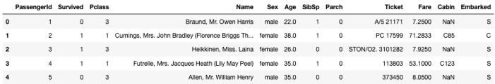
Here we have a mixture of features with categorical and numerical.
select
  quantified_features(
    ${output_row}, PassengerId, Survived, Pclass, Sex, Age, SibSp, Parch, Fare, Cabin, Embarked) as features
from (
  select * from titanic
  order by Passengerid asc
) t
limit 5;
and we get the following output
[1.0,0.0,0.0,3.0,0.0,22.0,1.0,0.0,7.25,0.0,1.0]
[2.0,1.0,1.0,1.0,1.0,38.0,1.0,0.0,71.2833,1.0,2.0]
[3.0,1.0,1.0,3.0,1.0,26.0,0.0,0.0,7.9250,0.0,1.0]
[4.0,1.0,1.0,1.0,1.0,35.0,1.0,0.0,53.1,3.0,1.0]
[5.0,1.0,0.0,3.0,0.0,35.0,0.0,0.0,8.05,0.0,1.0]
The ordering within the attributes is important, and some thinking is needed if there is a defined order and you want this reflected in the outputs of the transformed features
If you are a numeric field that you want treated as a categorical, and transformed, you can cast it into a string
e.g.
cast(SibSp as string)Python transforming Categorical to Numeric
When preparing data for input to machine learning algorithms you may have to perform certain types of data preparation.
In most enterprise solutions all or most of these tasks are automated for you, but in many languages they aren’t. The enterprise solutions are about ‘automating the boring stuff’ so that you don’t have to worry about it and waste valuable time doing boring, repetitive things.
The following examples illustrates a number of ways to record categorical variables into numeric. There are a number of approaches available, and it is up to you to decide which one might work best for your problem, your data, etc.
Let’s begin by loading the data set to be used in these examples. It is a Video Games reviews data set.
# perform some Statistics on the items in a panda
import pandas as pd
import numpy as np
import matplotlib as plt
videoReview = pd.read_csv('/Users/brendan.tierney/Downloads/Video_Games_Sales_as_at_22_Dec_2016.csv')
videoReview.head(10)

What are the data types of each variable
videoReview.dtypes

We don’t want to work with all the data in these examples. We just want to concentrate on the categorical variables. Let’s us create a subset of the dataframe to contains these.
df = videoReview.select_dtypes(include=['object']).copy()
df.head(10)

Now do a little data clean up by removing NaN (nulls)
df.dropna(inplace=True)
df.isnull().sum()

df.describe()

The above image shows the number of unique values in each of the variables. We will use Platform, Genre and Rating for the variable example below.
Let us chart these variables.
#check the number of passengars for each variable
import seaborn as sb
import matplotlib.pyplot as plt

plt.rcParams['figure.figsize'] = 10, 8

sb.countplot(x='Platform',data=df, palette='hls')

sb.countplot(x='Genre',data=df, palette='hls')

sb.countplot(x='Rating',data=df, palette='hls')

1-One-hot Coding
The first approach is to use the commonly used one-hot coding method. This will take a categorical variable and create a set of new variables corresponding with each distinct value in the variable, and then populate it with a binary value to indicate the original value.
#apply one-hot-coding to all the categorical variables
# and create a new dataframe to store the results

df2 = pd.get_dummies(df)
df2.head(10)

As you can see we now have 8138 variables in the pandas dataframe!
That is a lot and may not be workable for you. You may need to look at some feature reduction methods to reduce the number of variables.
2-Find and Replace
In this example we will simple replace the values with defined values.
Let’s have a look at values in the Ratings variable and their frequencies.
df['Rating'].value_counts()

The last 4 values listed have very small number of occurrences.
We will group these into having one value/category
find_replace = {"Rating" : {"E": 1, "T": 2, "M": 3, "E10+": 4, "EC": 5, "K-A": 5, "RP": 5, "AO": 5}}
df.replace(find_replace, inplace=True)
df.head(10)

Now plot the newly generated rating values and their frequencies.
sb.countplot(x='Rating',data=df, palette='hls')

3 – Label encoding
With this technique where each distinct value in a categorical variable is converted to a number.
In this scenario you don’t get to pick the numeric value assigned to the value. It is system determined.
#let's check the data types again
df.dtypes

Our categorical variables are of ‘object’ data type. We need to convert to a category data type.
In this example ‘Platform’ as it has a large-ish number of values and we want a quick way of converting them we can illustrate this by creating a new variable.
df["Platform_Category"] = df["Platform"].astype('category')
df.dtypes

Now convert this new variable to numeric.
df["Platform_Category"] = df["Platform_Category"].cat.codes
df.head(20)

The number assigned to the Platform_Category variable is based on the alphabetical ordering of the values in the Platform variable. For example,
df.groupby("Platform")["Platform"].count()

4-Using SciKit-Learn transform
SciKit-Learn has a number of functions to help with data encodings. The first one we will look at is the ‘fit_transform’ function.
This will perform a similar task to what we have seen in a previous example
#Let's use the fit_tranforms function to encode the Genre variable
from sklearn.preprocessing import LabelEncoder

le_make = LabelEncoder()
df["Genre_Code"] = le_make.fit_transform(df["Genre"])
df[["Genre", "Genre_Code"]].head(10)

And we can see this comparison when we look at the frequency counts.
df.groupby("Genre_Code")["Genre_Code"].count()

df.head(10)

And now we can drop the Genre variable from the dataframe as it is no longer needed. BUT you will need to have recorded the mapping between the original Genre values and the numeric values for future reference.
df = df.drop('Genre', axis=1)
df.head(10)

5-Using SciKit-Learn LabelEndcoder
SciKit-Learn has a binary label encoder and it can be used in a similar way to the previous example and also similar to the ‘get_dummies’ function.
from sklearn.preprocessing import LabelBinarizer

lb_style = LabelBinarizer()
lb_results = lb_style.fit_transform(df["Rating"])
lb_df = pd.DataFrame(lb_results, columns=lb_style.classes_)
lb_df.head(10)

These can now be joined with the original dataframe or a with a subset of the original dataframe to form a new dataframe consisting of the required variables.
As you can see, from the following, there are several other data pre-processing functions available in SciKit-Learn.

Data Normalization in Oracle Data Mining
Normalization is the process of scaling continuous values down to a specific range, often between zero and one. Normalization transforms each numerical value by subtracting a number, called the shift, and dividing the result by another number called the scale. The normalization techniques include:
- Min-Max Normalization : There is where the normalization is based on the using the minimum value for the shift and the (maximum-minimum) for the scale.
- Scale Normalization : This is where the normalization is based on zero being used for the shift and the value calculated using max[abs(max), abs(min)] being used for the scale
- Z-Score Normalization : This is where the normalization is based on using the mean value for the shift and the standard deviation for the scale.
When using Automatic Data Processing the normalization functions are used. But sometimes you may want to process the data is a more explicit manner. To do so you can use the various normalization function. To use these there is a three stage process. The first stage involves the creation of a table that will contain the normalization transformation data. The second stage applies the normalization procedures to your data source, defines the normalization required and inserts the required transformation data into the table create during the first stage. The third stage involves the defining of a view that applies the normalization transformations to your data source and displays the output via a database view. The following example illustrates how you can normalize the AGE and YRS_RESIDENCE attributes. The input data source will be the view that was created as the output of the previous transformation (MINING_DATA_V_2). This is passed on the original MINING_DATA_BUILD_V data set. The final output from this transformation step and all the other data transformation steps is MINING_DATA_READY_V.
BEGIN
   -- Clean-up : Drop the previously created tables
   BEGIN
      execute immediate 'drop table TRANSFORM_NORMALIZE';
   EXCEPTION
      WHEN others THEN
         null;
   END;

   -- Stage 1 : Create the table for the transformations
   -- Perform normalization for: AGE and YRS_RESIDENCE
   dbms_data_mining_transform.CREATE_NORM_LIN (
      norm_table_name => 'MINING_DATA_NORMALIZE');

   -- Step 2 : Insert the normalization data into the table
   dbms_data_mining_transform.INSERT_NORM_LIN_MINMAX (
      norm_table_name => 'MINING_DATA_NORMALIZE',
      data_table_name => 'MINING_DATA_V_2',
      exclude_list    => DBMS_DATA_MINING_TRANSFORM.COLUMN_LIST (
                         'affinity_card',
                         'bookkeeping_application',
                         'bulk_pack_diskettes',
                         'cust_id',
                         'flat_panel_monitor',
                         'home_theater_package',
                         'os_doc_set_kanji',
                         'printer_supplies',
                         'y_box_games'));

   -- Stage 3 : Create the view with the transformed data
   DBMS_DATA_MINING_TRANSFORM.XFORM_NORM_LIN (
      norm_table_name => 'MINING_DATA_NORMALIZE',
      data_table_name => 'MINING_DATA_V_2',
      xform_view_name => 'MINING_DATA_READY_V');

END;
/
The above example performs normalization based on the Minimum-Maximum values of the variables/columns. The other normalization functions are:
| INSERT_NORM_LIN_SCALE | Inserts linear scale normalization definitions in a transformation definition table. |
| INSERT_NORM_LIN_ZSCORE | Inserts linear zscore normalization definitions in a transformation definition table. |
Hivemall: Feature Scaling based on Min-Max values
Once of the most common tasks when preparing data for data mining and machine learning is to take numerical data and scale it. Most enterprise and advanced tools and languages do this automatically for you, but with lower level languages you need to perform the task. There are a number of approaches to doing this. In this example we will use the Min-Max approach.
With the Min-Max feature scaling approach, we need to find the Minimum and Maximum values of each numerical feature. Then using a scaling function that will re-scale the data to a Zero to One range. The general formula for this is.

Using the IRIS data set as the data set (and loaded in previous post), the first thing we need to find is the minimum and maximum values for each feature.
select min(features[0]), max(features[0]),
       min(features[1]), max(features[1]),
       min(features[2]), max(features[2]),
       min(features[3]), max(features[3])
from iris_raw;
we get the following results.
4.3 7.9 2.0 4.4 1.0 6.9 0.1 2.5
The format of the results can be a little confusing. What this list gives us is the results for each of the four features.
For feature[0], sepal_length, we have a minimum value of 4.3 and a maximum value of 7.9.
Similarly,
feature[1], sepal_width, min=2.0, max=4.4
feature[2], petal_length, min=1.0, max=6.9
feature[3], petal_width, min=0.1, max=2.5
To use these minimum and maximum values, we need to declare some local session variables to store these.
set hivevar:feature0_min=4.3;
set hivevar:feature0_max=7.9;
set hivevar:feature1_min=2.0;
set hivevar:feature1_max=4.4;
set hivevar:feature2_min=1.0;
set hivevar:feature2_max=6.9;
set hivevar:feature3_min=0.1;
set hivevar:feature3_max=2.5;
After setting those variables we can now write a SQL SELECT and use the add_bias function to perform the calculations.
select rowid, label,
       add_bias(array(
          concat("1:", rescale(features[0],${f0_min},${f0_max})),
          concat("2:", rescale(features[1],${f1_min},${f1_max})),
          concat("3:", rescale(features[2],${f2_min},${f2_max})),
          concat("4:", rescale(features[3],${f3_min},${f3_max})))) as features
from iris_raw;
and we get
> 1 Iris-setosa   ["1:0.22222215","2:0.625","3:0.0677966","4:0.041666664","0:1.0"]
> 2 Iris-setosa   ["1:0.16666664","2:0.41666666","3:0.0677966","4:0.041666664","0:1.0"]
> 3 Iris-setosa   ["1:0.11111101","2:0.5","3:0.05084745","4:0.041666664","0:1.0"]
...
Other feature scaling methods, available in Hivemall, include L1/L2 Normalization and zscore.
OCI – Making DBaaS Accessible using port 1521
When setting up a Database on Oracle Cloud Infrastructure (OCI) for the first time there are a few pre and post steps to complete before you can access the database using a JDBC type of connect, just like what you have in SQL Developer, or using Python or other similar tools and/or languages.
1. Setup Virtual Cloud Network (VCN)
The first step, when starting off with OCI, is to create a Virtual Cloud Network.
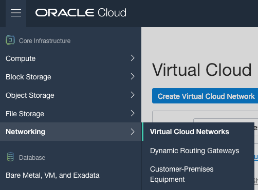
Create a VCN and take all the defaults. But change the radio button shown in the following image.
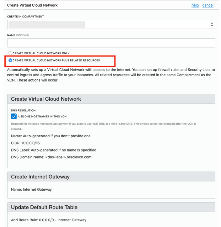
That’s it. We will come back to this later.
2. Create the Oracle Database
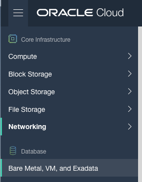
To create the database select ‘Bare Metal, VM and Exadata’ from the menu.
Click on the ‘Launch DB System’ button.
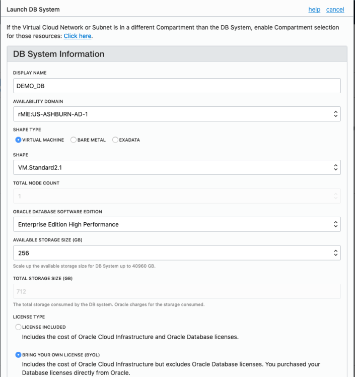
Fill in the details of the Database you want to create and select from the various options from the drop-downs.
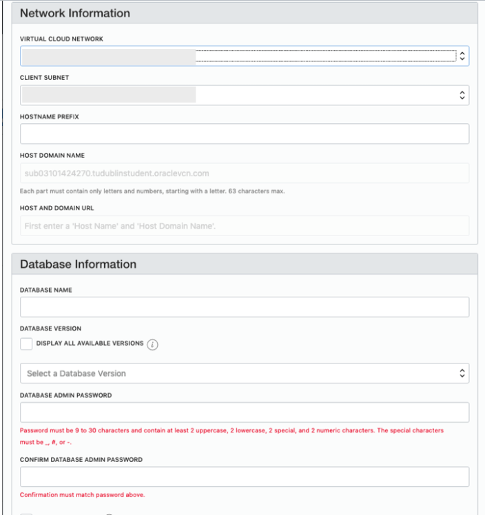
Fill in the details of the VCN you created in the previous set, and give the name of the DB and the Admin password.
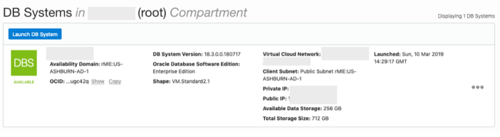
When you are finished everything that is needed, the ‘Launch DB System’ at the bottom of the page will be enabled. After clicking on this botton, the VM will be built and should be ready in a few minutes. When finished you should see something like this.
3. SSH to the Database server
When the DB VM has been created you can now SSH to it. You will need to use the SSH key file used when creating the DB VM. You will need to connect to the opc (operating system user), and from there sudo to the oracle user. For example
ssh -i <ssh file> opc@<public IP address>
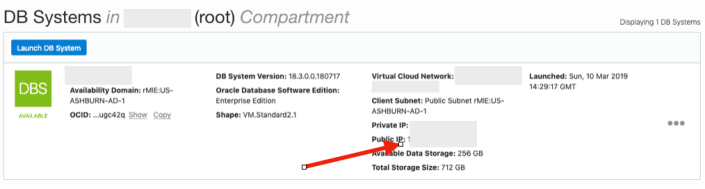
The public IP address can be found with the Database VM details
[opc@tudublins1 ~]$ sudo su - oracle
[oracle@tudublins1 ~]$ . oraenv
ORACLE_SID = [cdb1] ?
The Oracle base has been set to /u01/app/oracle
[oracle@tudublins1 ~]$
[oracle@tudublins1 ~]$ sqlplus / as sysdba

SQL*Plus: Release 18.0.0.0.0 - Production on Wed Mar 13 11:28:05 2019
Version 18.3.0.0.0

Copyright (c) 1982, 2018, Oracle. All rights reserved.


Connected to:
Oracle Database 18c Enterprise Edition Release 18.0.0.0.0 - Production
Version 18.3.0.0.0

SQL> alter session set container = pdb1;

Session altered.

SQL> create user demo_user identified by DEMO_user123##;

User created.

SQL> grant create session to demo_user;

Grant succeeded.

SQL>
4. Open port 1521
To be able to access this with a Basic connection in SQL Developer and most programming languages, we will need to open port 1521 to allow these tools and languages to connect to the database.
To do this go back to the Virtual Cloud Networks section from the menu.
Click into your VCN, that you created earlier. You should see something like the following.
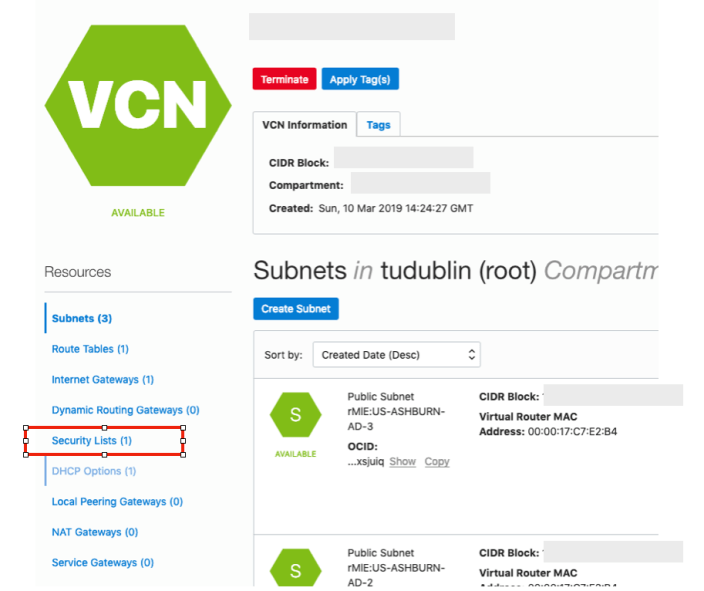
Click on the Security Lists, menu option on the left hand side.
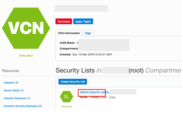 From that screen, click on Default Security List, and then click on the ‘Edit All Rules’ button at the top of the next screen.
Add a new rule to have a ‘Destination Port Range’ set for 1521
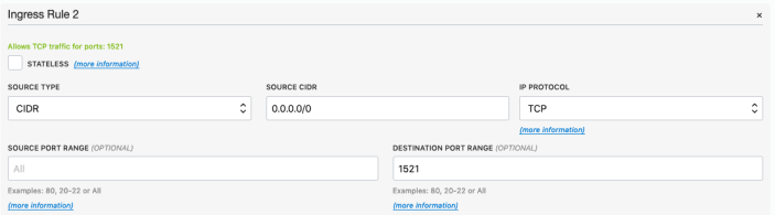
That’s it.
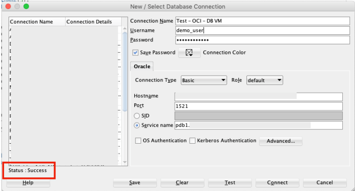
5. Connect to the Database from anywhere
Now you can connect to the OCI Database using a basic SQL Developer Connection.
HiveMall: Docker image setup
In a previous blog post I introduced HiveMall as a SQL based machine learning language available for Hadoop and integrated with Hive.
If you have your own Hadoop/Big Data environment, I provided the installation instructions for Hivemall, in that blog post
An alternative is to use Docker. There is a HiveMall Docker image available. A little warning before using this image. It isn’t updated with the latest release but seems to get updated twice a year. Although you may not be running the latest version of HiveMall, you will have a working environment that will have almost all the functionality, bar a few minor new features and bug fixes.
To get started, you need to make sure you have Docker running on your machine and you have logged into your account. The docker image is available from Docker Hub. Take note of the version number for the latest version of the docker image. In this example it is 20180924

Open a terminal window and run the following command. This will download and extract all the image files.
docker pull hivemall/latest:20180924
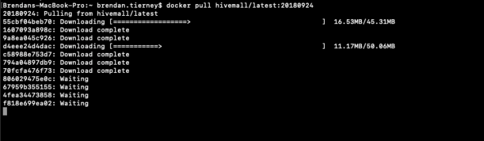
Until everything is completed.
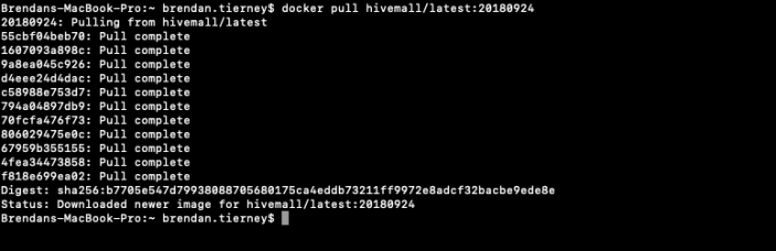
This docker image has HDFS, Yarn and MapReduce installed and running. This will require the exposing of the ports for these services 8088, 50070 and 19888.
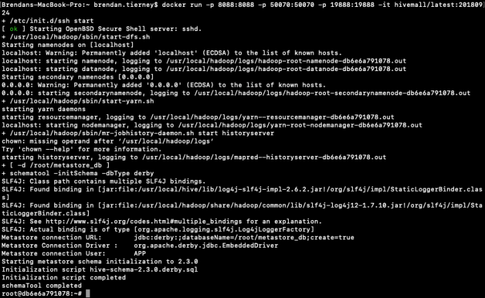
To start the HiveMall docker image run
docker run -p 8088:8088 -p 50070:50070 -p 19888:19888 -it hivemall/latest:20180924Consider creating a shell script for this, to make it easier each time you want to run the image.
Now seed Hive with some data. The typical example uses the IRIS data set. Run the following command to do this. This script downloads the IRIS data set, creates a number directories and then creates an external table, in Hive, to point to the IRIS data set.
cd $HOME && ./bin/prepare_iris.sh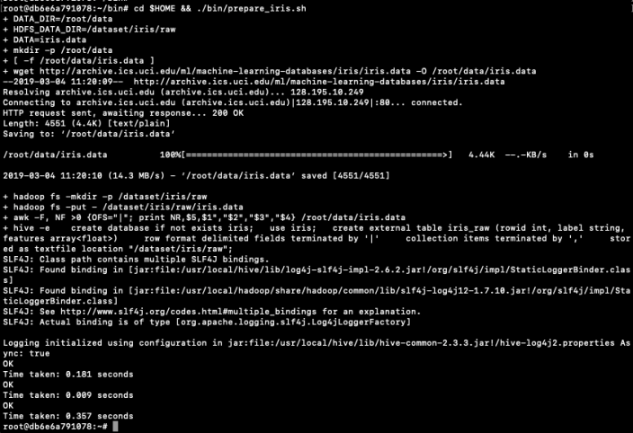
Now open Hive and list the databases.
hive -S
hive> show databases;
OK
default
iris
Time taken: 0.131 seconds, Fetched: 2 row(s)
Connect to the IRIS database and list the tables within it.
hive> use iris;
hive> show tables;
iris_raw
Now query the data (150 records)
hive> select * from iris_raw;
1 Iris-setosa [5.1,3.5,1.4,0.2]
2 Iris-setosa [4.9,3.0,1.4,0.2]
3 Iris-setosa [4.7,3.2,1.3,0.2]
4 Iris-setosa [4.6,3.1,1.5,0.2]
5 Iris-setosa [5.0,3.6,1.4,0.2]
6 Iris-setosa [5.4,3.9,1.7,0.4]
7 Iris-setosa [4.6,3.4,1.4,0.3]
8 Iris-setosa [5.0,3.4,1.5,0.2]
9 Iris-setosa [4.4,2.9,1.4,0.2]
10 Iris-setosa [4.9,3.1,1.5,0.1]
11 Iris-setosa [5.4,3.7,1.5,0.2]
12 Iris-setosa [4.8,3.4,1.6,0.2]
13 Iris-setosa [4.8,3.0,1.4,0.1
...
Find the min and max values for each feature.
hive> select
    > min(features[0]), max(features[0]),
    > min(features[1]), max(features[1]),
    > min(features[2]), max(features[2]),
    > min(features[3]), max(features[3])
    > from
    > iris_raw;

4.3  7.9  2.0  4.4  1.0  6.9  0.1  2.5
You are now up and running with HiveMall on Docker.
Ethics in the AI, Machine Learning, Data Science, etc Era
Ethics is one of those topics that everyone has a slightly different definition or view of what it means. The Oxford English dictionary defines ethics as, ‘Moral principles that govern a person’s behaviour or the conducting of an activity‘.
As you can imagine this topic can be difficult to discuss and has many, many different aspects.
In the era of AI, Machine Learning, Data Science, etc the topic of Ethics is finally becoming an important topic. Again there are many perspective on this. I’m not going to get into these in this blog post, because if I did I could end up writing a PhD dissertation on it.
But if you do work in the area of AI, Machine Learning, Data Science, etc you do need to think about the ethical aspects of what you do. For most people, you will be working on topics where ethics doesn’t really apply. For example, examining log data, looking for trends, etc
But when you start working of projects examining individuals and their behaviours then you do need to examine the ethical aspects of such work. Everyday we experience adverts, web sites, marketing, etc that has used AI, Machine Learning and Data Science to delivery certain product offerings to us.
Just because we can do something, doesn’t mean we should do it.

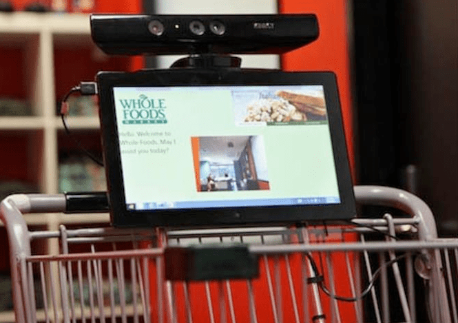
One particular area that I will not work on is Location Based Advertising. Imagine walking down a typical high street with lots and lots of retail stores. Your phone vibrates and on the screen there is a message. The message is a special offer or promotion for one of the shops a short distance ahead of you. You are being analysed. Your previous buying patterns and behaviours are being analysed, Your location and direction of travel is being analysed. Some one, or many AI applications are watching you. This is not anything new and there are lots of examples of this from around the world.

But what if this kind of Location Based Advertising was taken to another level. What if the shops had cameras that monitored the people walking up and down the street. What if those cameras were analysing you, analysing what clothes you are wearing, analysing the brands you are wearing, analysing what accessories you have, analysing your body language, etc. They are trying to analyse if you are the kind of person they want to sell to. They then have staff who will come up to you, as you are walking down the street, and will have customised personalised special offers on products in their store, just for you.
See the segment between 2:00 and 4:00 in this video. This gives you an idea of what is possible.
Are you Ok with this?
As an AI, Machine Learning, Data Science professional, are you Ok with this?
The technology exists to make this kind of Location Based Marketing possible. This will be an increasing ethical consideration over the coming years for those who work in the area of AI, Machine Learning, Data Science, etc
Just because we can, doesn’t mean we should!

You must be logged in to post a comment.