
12c
RandomForest Machine Learning – Oracle Machine Learning (OML)
Oracle Machine Learning has 30+ different machine learning algorithms built into the database. This means you can use SQL to create machine learning models and then use these models to score or label new data stored in the database or as the data is being created dynamically in the applications.
One of the most commonly used machine learning algorithms, over the past few years, is can RandomForest. This post will take a closer look at this algorithm and how you can build & use a RandomForest model.
Random Forest is known as an ensemble machine learning technique that involves the creation of hundreds of decision tree models. These hundreds of models are used to label or score new data by evaluating each of the decision trees and then determining the outcome based on the majority result from all the decision trees. Just like in the game show. The combining of a number of different ways of making a decision can result in a more accurate result or prediction.
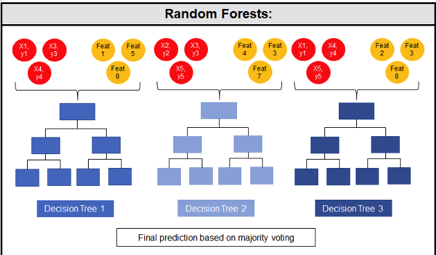
Random Forest models can be used for classification and regression types of problems, which form the majority of machine learning systems and solutions. For classification problems, this is where the target variable has either a binary value or a small number of defined values. For classification problems the Random Forest model will evaluate the predicted value for each of the decision trees in the model. The final predicted outcome will be the majority vote for all the decision trees. For regression problems the predicted value is numeric and on some range or scale. For example, we might want to predict a customer’s lifetime value (LTV), or the potential value of an insurance claim, etc. With Random Forest, each decision tree will make a prediction of this numeric value. The algorithm will then average these values for the final predicted outcome.
Under the hood, Random Forest is a collection of decision trees. Although decision trees are a popular algorithm for machine learning, they can have a tendency to over fit the model. This can lead higher than expected errors when predicting unseen data. It also gives just one possible way of representing the data and being able to derive a possible predicted outcome.
 Random Forest on the other hand relies of the predicted outcomes from many different decision trees, each of which is built in a slightly different way. It is an ensemble technique that combines the predicted outcomes from each decision tree to give one answer. Typically, the number of trees created by the Random Forest algorithm is defined by a parameter setting, and in most languages this can default to 100+ or 200+ trees.
The Random Forest algorithm has three main features:
- It uses a method called bagging to create different subsets of the original training data
- It will randomly section different subsets of the features/attributes and build the decision tree based on this subset
- By creating many different decision trees, based on different subsets of the training data and different subsets of the features, it will increase the probability of capturing all possible ways of modeling the data
For each decision tree produced, the algorithm will use a measure, such as the Gini Index, to select the attributes to split on at each node of the decision tree.
To create a RandomForest model using Oracle Data Mining, you will follow the same process as with any of the other algorithms, the core of these are:
- define the parameter settings
- create the model
- score/label new data
Let’s start with the first step, defining the parameters. As with all the classification algorithms the same or similar parameters are set. With RandomForest we can set an additional parameter which tells the algorithm how many decision trees to create as part of the model. By default, 20 decision trees will be created. But if you want to change this number you can use the RFOR_NUM_TREES parameter. Remember the larger the value the longer it will take to create the model. But will have better accuracy. On the other hand with a small number of trees the quicker the model build will be, but might night be as accurate. This is something you will need to explore and determine. In the following example I change the number of trees to created to ten.
CREATE TABLE BANKING_RF_SETTINGS (
    SETTING_NAME VARCHAR2(50),
    SETTING_VALUE VARCHAR2(50)
);

BEGIN
  DELETE FROM BANKING_RF_SETTINGS;

  INSERT INTO banking_RF_settings (setting_name, setting_value)
  VALUES (dbms_data_mining.algo_name, dbms_data_mining.algo_random_forest);

  INSERT INTO banking_RF_settings (setting_name, setting_value)
  VALUES (dbms_data_mining.prep_auto, dbms_data_mining.prep_auto_on);

  INSERT INTO banking_RF_settings (setting_name, setting_value)
  VALUES (dbms_data_mining.RFOR_NUM_TREES, 10);

  COMMIT;
END;
Other default parameters used include, for creating each decision tree, use random 50% selection of columns and 50% sample of training data.
Now for step 2, create the model.
DECLARE
   v_start_time  TIMESTAMP;
BEGIN
   DBMS_DATA_MINING.DROP_MODEL('BANKING_RF_72K_1');

   v_start_time := current_timestamp;

   DBMS_DATA_MINING.CREATE_MODEL(
      model_name          => 'BANKING_RF_72K_1',
      mining_function     => dbms_data_mining.classification,
      data_table_name     => 'BANKING_72K',
      case_id_column_name => 'ID',
      target_column_name  => 'TARGET',
      settings_table_name => 'BANKING_RF_SETTINGS');

   dbms_output.put_line('Time take to create model = ' || to_char(extract(second from (current_timestamp-v_start_time))) || ' seconds.');
END;
The above code measures how long it takes to create the model.
I’ve run this same parameters and create models for different training data set sizes. I’ve also changed the number of decision trees to create. The following table shows the timings.
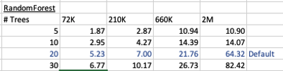
You can see it took 5.23 seconds to create a RandomForest model using the default settings for a data set of 72K records. This increase to just over one minute for a data set of 2 million records. Yo can also see the effect of reducing the number of decision trees on how long it takes the create model to run.
For step 3, on using the model on new data, this is just the same as with any of the classification models. Here is an example:
SELECT cust_id, target,
       prediction(BANKING_RF_72K_1 USING *)  predicted_value,
       prediction_probability(BANKING_RF_72K_1 USING *) probability
FROM   bank_test_v;
That’s it. That’s all there is to creating a RandomForest machine learning model using Oracle Machine Learning.
It’s quick and easy 🙂
Auto enabling APPROX_* function in the Oracle Database
With the releases of 12.1 and 12.2 of Oracle Database we have seen some new functions that perform approximate calculations. These include:
- APPROX_COUNT_DISTINCT
- APPROX_COUNT_DISTINCT_DETAIL
- APPROX_COUNT_DISTINCT_AGG
- APPROX_MEDIAN
- APPROX_PERCENTILE
- APPROX_PERCENTILE_DETAIL
- APPROX_PERCENTILE_AGG
These functions can be used when approximate answers can be used instead of the exact answer. Yes can have many scenarios for these and particularly as we move into the big data world, the ability to process our data quickly is slightly more important and exact numbers. For example, is there really a difference between 40% of our customers being of type X versus 41%. The real answer to this is, ‘It Depends!’, but for a lot of analytical and advanced analytical methods this difference doesn’t really make a difference.
There are various reports of performance improvement of anything from 6x to 50x with the response times of the queries that are using these functions, instead of using the more traditional functions.
If you are a BI or big data analyst and you have build lots of code and queries using the more traditional functions. But what if you now want to use the newer functions. Does this mean you have go and modify all the code you have written over the years? you can imagine getting approval to do this!
The simple answer to this question is ‘No’. No you don’t have to change any code, but with some parameter changes for the DB or your session you can tell the database to automatically switch from using the traditional functions (count, etc) to the newer more optimised and significantly faster APPROX_* functions.
So how can you do this magic?
First let us see what the current settings values are:
SELECT name, value
FROM   v$ses_optimizer_env
WHERE  sid = sys_context('USERENV','SID')
AND    name like '%approx%';

Now let us run a query to test what happens using the default settings (on a table I have with 10,500 records).
set auto trace on

select count(distinct cust_id) from test_inmemory;

COUNT(DISTINCTCUST_ID)
----------------------
		  1500


Execution Plan
----------------------------------------------------------
Plan hash value: 2131129625

--------------------------------------------------------------------------------------
| Id  | Operation	     | Name	     | Rows  | Bytes | Cost (%CPU)| Time     |
--------------------------------------------------------------------------------------
|   0 | SELECT STATEMENT     |		     |	   1 |	  13 |	  70   (2)| 00:00:01 |
|   1 |  SORT AGGREGATE      |		     |	   1 |	  13 |		  |	     |
|   2 |   VIEW		     | VW_DAG_0      |	1500 | 19500 |	  70   (2)| 00:00:01 |
|   3 |    HASH GROUP BY     |		     |	1500 |	7500 |	  70   (2)| 00:00:01 |
|   4 |     TABLE ACCESS FULL| TEST_INMEMORY | 10500 | 52500 |	  69   (0)| 00:00:01 |
--------------------------------------------------------------------------------------
Let us now set the automatic usage of the APPROX_* function.
alter session set approx_for_aggregation = TRUE;

SQL> select count(distinct cust_id) from test_inmemory;

COUNT(DISTINCTCUST_ID)
----------------------
		  1495


Execution Plan
----------------------------------------------------------
Plan hash value: 1029766195

---------------------------------------------------------------------------------------
| Id  | Operation	      | Name	      | Rows  | Bytes | Cost (%CPU)| Time     |
---------------------------------------------------------------------------------------
|   0 | SELECT STATEMENT      | 	      |     1 |     5 |    69	(0)| 00:00:01 |
|   1 |  SORT AGGREGATE APPROX| 	      |     1 |     5 | 	   |	      |
|   2 |   TABLE ACCESS FULL   | TEST_INMEMORY | 10500 | 52500 |    69	(0)| 00:00:01 |
---------------------------------------------------------------------------------------
We can see above that the APPROX_* equivalent function was used, and slightly less work. But we only used this on a very small table.
The full list of session level settings is:
alter session set approx_for_aggregation = TRUE;
alter session set approx_for_aggregation = FALSE;

alter session set approx_for_count_distinct = TRUE;
alter session set approx_for_count_distinct = FALSE;

alter session set approx_for_percentile = 'PERCENTILE_CONT DETERMINISTIC';
alter session set approx_for_percentile = PERCENTILE_DISC;
alter session set approx_for_percentile = NONE;
Or at a system wide level:
alter system set approx_for_aggregation = TRUE;
alter system set approx_for_aggregation = FALSE;

alter system set approx_for_count_distinct = TRUE;
alter system set approx_for_count_distinct = FALSE;

alter system set approx_for_percentile = 'PERCENTILE_CONT DETERMINISTIC';
alter system set approx_for_percentile = PERCENTILE_DISC;
alter system set approx_for_percentile = NONE;
And to reset back to the default settings:
alter system reset approx_for_aggregation;
alter system reset approx_for_count_distinct;
alter system reset approx_for_percentile;
Setting up Oracle Database on Docker
A couple of days ago it was announced that several Oracle images were available on the Docker Store.
This is by far the easiest Oracle Database install I have every done !
You simply have no excuse now for not installing and using an Oracle Database. Just go and do it now!
The following steps outlines what I did you get an Oracle 12.1c Database.
1. Download and Install Docker
There isn’t much to say here. Just go to the Docker website, select the version docker for your OS, and just install it.
You will probably need to create an account with Docker.

After Docker is installed it will automatically start and and will be placed in your system tray etc so that it will automatically start each time you restart your laptop/PC.
2. Adjust the memory allocation
From the system tray open the Docker application. In the Advanced section allocate a bit more memory. This will just make things run a bit smoother. Be a bit careful on how much to allocate.

In the General section check the tick-box for automatically backing up Docker VMs. This is assuming you have back-ups setup, for example with Time Machine or something similar.
3. Download & Edit the Oracle Docker environment File
On the Oracle Database download Docker webpage, click on the the Get Content button.

You will have to enter some details like your name, company, job title and phone number, then click on the check-box, before clicking on the Get Content button. All of this is necessary for the Oracle License agreement.
The next screen lists the Docker Services and Partner Services that you have signed up for.

Click on the Setup button to go to the webpage that contains some of the setup instructions.

The first thing you need to do is to copy the sample Environment File. Create a new file on your laptop/desktop and paste the environment file contents into the file. There are a few edits you need to make to this file. The following is the edited/modified Environment file that I created and used. The changes are for DB_SID, DB_PASSWD and DB_DOMAIN.
####################################################################
## Copyright(c) Oracle Corporation 1998,2016. All rights reserved.##
##                                                                ##
##                   Docker OL7 db12c dat file                    ##
##                                                                ##
####################################################################

##------------------------------------------------------------------
## Specify the basic DB parameters
##------------------------------------------------------------------

## db sid (name)
## default : ORCL
## cannot be longer than 8 characters

DB_SID=ORCL

## db passwd
## default : Oracle

DB_PASSWD=oracle

## db domain
## default : localdomain

DB_DOMAIN=localdomain

## db bundle
## default : basic
## valid : basic / high / extreme
## (high and extreme are only available for enterprise edition)

DB_BUNDLE=basic

## end
I called this file ‘docker_ora_db.txt‘
4. Download and Configure Oracle Database for Docker
The following command will download and configure the docker image
$ docker run -d --env-file ./docker_ora_db.txt -p 1527:1521 -p 5507:5500 -it --name dockerDB121 --shm-size="8g" store/oracle/database-enterprise:12.1.0.2
This command will create a container called ‘dockerDB121’. The 121 at the end indicate the version number of the Oracle Database. If you end up with a number of containers containing different versions of the Oracle Database then you need some way of distinguishing them.
Take note of the port mapping in the above command, as you will need this information later.
When you run this command, the docker image will be downloaded from the docker website, will be unzipped and the container setup and ready to run.

5. Log-in and Finish the configuration
Although the docker container has been setup, there is still a database configuration to complete. The following images shows that the new containers is there.

To complete the Database setup, you will need to log into the Docker container.
docker exec -it dockerDB121 /bin/bash
Then run the Oracle Database setup and startup script (as the root user).
/bin/bash /home/oracle/setup/dockerInit.sh

This script can take a few minutes to run. On my laptop it took about 2 minutes.
When this is finished the terminal session will open as this script goes into a look.
To run any other commands in the container you will need to open another terminal session and connect to the Docker container. So go open one now.
6. Log into the Database in Docker
In a new terminal window, connect to the Docker container and then switch to the oracle user.
su - oracle
Check that the Oracle Database processes are running (ps -ef) and then connect as SYSDBA.
sqlplus / as sysdba
Let’s check out the Database.
SQL> select name,DB_UNIQUE_NAME from v$database;

NAME	  DB_UNIQUE_NAME
--------- ------------------------------
ORCL	  ORCL


SQL> SELECT v.name, v.open_mode, NVL(v.restricted, 'n/a') "RESTRICTED", d.status
     FROM v$pdbs v, dba_pdbs d
     WHERE v.guid = d.guid
     ORDER BY v.create_scn;


NAME			       OPEN_MODE  RES STATUS
------------------------------ ---------- --- ---------
PDB$SEED		       READ ONLY  NO  NORMAL
PDB1			       READ WRITE NO  NORMAL
And the tnsnames.ora file contains the following:
ORCL =   (DESCRIPTION =
    (ADDRESS = (PROTOCOL = TCP)(HOST = 0.0.0.0)(PORT = 1521))
     (CONNECT_DATA =
      (SERVER = DEDICATED)
       (SERVICE_NAME = ORCL.localdomain)     )   )

PDB1 =   (DESCRIPTION =
     (ADDRESS = (PROTOCOL = TCP)(HOST = 0.0.0.0)(PORT = 1521))
      (CONNECT_DATA =
       (SERVER = DEDICATED)
       (SERVICE_NAME = PDB1.localdomain)     )   )
You are now up an running with an Docker container running an Oracle 12.1 Databases.
7. Configure SQL Developer (on Client) to
access the Oracle Database on Docker
You can not use your client tools to connect to the Oracle Database in a Docker Container. Here is a connection setup in SQL Developer.

Remember that port number mapping I mentioned in step 4 above. See in this SQL Developer connection that the port number is 1527.
Thats it. How easy is that. You now have a fully configured Oracle 12.1c Enterprise Edition Database to play with, to have fun and to explore all the wonderful features of the Oracle Database.
PREDICTION_DETAILS function in Oracle
When building predictive models the data scientist can spend a large amount of time examining the models produced and how they work and perform on their hold out sample data sets. They do this to understand is the model gives a good general representation of the data and can identify/predict many different scenarios. When the “best” model has been selected then this is typically deployed is some sort of reporting environment, where a list is produced. This is typical deployment method but is far from being ideal. A more ideal deployment method is that the predictive models are build into the everyday applications that the company uses. For example, it is build into the call centre application, so that the staff have live and real-time feedback and predictions as they are talking to the customer.
But what kind of live and real-time feedback and predictions are possible. Again if we look at what is traditionally done in these applications they will get a predicted outcome (will they be a good customer or a bad customer) or some indication of their value (maybe lifetime value, possible claim payout value) etc.
But can we get anymore information? Information like what was reason for the prediction. This is sometimes called prediction insight. Can we get some details of what the prediction model used to decide on the predicted value. In more predictive analytics products this is not possible, as all you are told is the final out come.
What would be useful is to know some of the thinking that the predictive model used to make its thinking. The reasons when one customer may be a “bad customer” might be different to that of another customer. Knowing this kind of information can be very useful to the staff who are dealing with the customers. For those who design the workflows etc can then build more advanced workflows to support the staff when dealing with the customers.
Oracle as a unique feature that allows us to see some of the details that the prediction model used to make the prediction. This functions (based on using the Oracle Advanced Analytics option and Oracle Data Mining to build your predictive model) is called PREDICTION_DETAILS.
When you go to use PREDICTION_DETAILS you need to be careful as it will work differently in the 11.2g and 12c versions of the Oracle Database (Enterprise Editions). In Oracle Database 11.2g the PREDICTION_DETAILS function would only work for Decision Tree models. But in 12c (and above) it has been opened to include details for models created using all the classification algorithms, all the regression algorithms and also for anomaly detection.
The following gives an example of using the PREDICTION_DETAILS function.
select cust_id,
       prediction(clas_svm_1_27 using *) pred_value,
       prediction_probability(clas_svm_1_27 using *) pred_prob,
       prediction_details(clas_svm_1_27 using *) pred_details
from mining_data_apply_v;
The PREDICTION_DETAILS function produces its output in XML, and this consists of the attributes used and their values that determined why a record had the predicted value. The following gives some examples of the XML produced for some of the records.

I’ve used this particular function in lots of my projects and particularly when building the applications for a particular business unit. Oracle too has build this functionality into many of their applications. The images below are from the HCM application where you can examine the details why an employee may or may not leave/churn. You can when perform real-time what-if analysis by changing some of attribute values to see if the predicted out come changes.

Loading JSON data into Oracle using ROracle and jsonlite
In this post I want to show you one way of taking a JSON file of data and loading it into your Oracle schema using ROracle. The JSON data will then be used to create a table in your schema. Yes you could use other methods to connect to the database and to create the table. But ROracle is by far the fastest method of connecting, selecting and processing data.
1. Necessary R Packages
You will need two R library. The first of these is the ROracle package. This gives us all the connection and data processing commands to work with the Oracle database. The second package is the jsonlite R package. This package allows us to open, read and process a file that has JSON data.
> install.package(“ROracle”)
> install.package(“jsonlite”)
After you have installed the packages you can now load them into your R environment so that you can use them in your current session.
> library(ROracle)
> library(jsonlite)
Depending on your version of R you may get some working messages about the libraries being built under a different version of R. Then again maybe you won’t get these 🙂
2. Open & Read the JSON file in R
Now you are ready to name and open the file that contains your JSON data. In my case the file is called ‘demo_json_data.json’
> jsonFile <- "c:/app/demo_json_data.json"
> jsonData <- fromJSON(jsonFile)
We now have the JSON data loaded into R. We can now look at the attributes of each JSON record and the number of records that was in the JSON file.
> names(jsonData$items)
[1] “cust_id” “cust_gender” “age”
[4] “cust_marital_status” “country_name” “cust_income_level”
[7] “education” “occupation” “household_size”
[10] “yrs_residence” “affinity_card” “bulk_pack_diskettes”
[13] “flat_panel_monitor” “home_theater_package” “bookkeeping_application”
[16] “printer_supplies” “y_box_games” “os_doc_set_kanji”
> nrow(jsonData$items)
[1] 1500
As you can see the records are grouped under a higher label of ‘items’. You might want to extract these records into a new data frame.
> data <- jsonData$items
>
Now we have our data ready in a data frame and we can use this data frame to create a table and insert the data.
3. Create the connection to the Oracle Schema
I have a previous post on connecting to an Oracle Schema using ROracle. That was connecting to an 11g Oracle Database.
JSON is a new feature in Oracle 12c and the connection details are a little bit different because we are now having to deal with connection to a pluggable database. The following illustrates connecting to a 12c database and assumes you have Oracle Client already installed and configured with your tnsnames.ora entry.
# Create the connection string
> host <- "localhost"
> port <- 1521
> service <- "pdb12c"
> connect.string <- paste(
“(DESCRIPTION=”,
“(ADDRESS=(PROTOCOL=tcp)(HOST=”, host, “)(PORT=”, port, “))”,
“(CONNECT_DATA=(SERVICE_NAME=”, service, “)))”, sep = “”)
> con2 <- dbConnect(drv, username = "dmuser", password = "dmuser",dbname=connect.string)
>
4. Create the table in your Oracle Schema
At this point we have our connection to our Oracle Schema setup and connected, we have read in the JSON file and we have the JSON data in a data frame. We are now ready to push the JSON data to a table in our schema.
> dbWriteTable(con, “JSON_DATA”, overwrite=TRUE, value=data)
Job done 🙂
The table JSON_DATA has been created and the data is stored in the table in typical table attributes and rows format.
One thing to watch our for with the above command is with the overwrite=TRUE parameter setting. This replaces a table if it already exists. So your old data will be gone. Be careful.
5. View and Query the data using SQL
When you now log into your schema in the 12c Database, you can now query the data in the JSON_DATA table. (Yes I know it is not in JSON format in this table).

How did I get/generate my JSON data?
I generated the JSON file using a table that I already had in one of my schemas. This table is part of the sample data set that is built on top of the Oracle sample schemas.
The image below shows the steps involved in generating the data in JSON format. I used SQL Developer and set the SQLFORMAT to be JSON. I then ran the query to select the data. You will need to run this as a script. Then copy the JSON data and paste it into a file.

The SQL FORMAT command sets the output format for a query back to the default query output format that we are well use to.
A nice little JSON viewer can be found at http://jsonviewer.stack.hu/
Copy and paste your JSON data into this and you can view the structure of the data. Check it out.
Oracle Data Miner (ODM 4.1) New Features
With the release of SQL Developer 4.1 we also get a number of new features with Oracle Data Miner (ODMr). These include:
- Data Source node can now include data sources that contain JSON data, generating JSON schema and has a JSON viewer
- Create Table can now create data in JSON
- JSON Query Node allows you to view, query and process JSON data, combine it with relational data, generate sub-group by, and nested columns to be part of input to algorithms
- New PL/SQL APIs for managing Data Miner projects and workflows. This includes run, cancel, rename, delete, import and export of workflows using PL/SQL.
- New ODMr Repository views that allows us to query and monitor our workflows.
- Transformation Node now allows you different ways of handling NULLS.
- Transformation Node now allows us to create Custom Bins, define bin labels and bin values
- Overall Workflow and ODMr environment improvements to allow for greater efficiency in workflow behaviour and interactions with the database. So using ODMr should feel quicker and more responsive.
What out for the Gotchas: Although support for JSON has been added to ODMr, as outlined above, you are still a bit limited to what else you can do with your JSON data. Based on the documentation you can use JSON data in the Association and Classification build nodes.
I’m not sure about the other nodes and this will need a bit of investigation to see what nodes can and cannot use JSON data. I’m sure this will all be sorted out in the next release.
Keep an eye out for some blog posts over the coming weeks on how to explore and use these new features of Oracle Data Miner.
Viewing Models Details for Decision Trees using SQL
When you are working with and developing Decision Trees by far the easiest way to visualise these is by using the Oracle Data Miner (ODMr) tool that is part of SQL Developer.
Developing your Decision Tree models using the ODMr allows you to explore the decision tree produced, to drill in on each of the nodes of the tree and to see all the statistics etc that relate to each node and branch of the tree.
But when you are working with the DBMS_DATA_MINING PL/SQL package and with the SQL commands for Oracle Data Mining you don’t have the same luxury of the graphical tool that we have in ODMr. For example here is an image of part of a Decision Tree I have and was developed using ODMr.
What if we are not using the ODMr tool? In that case you will be using SQL and PL/SQL. When using these you do not have luxury of viewing the Decision Tree.
So what can you see of the Decision Tree? Most of the model details can be used by a variety of functions that can apply the model to your data. I’ve covered many of these over the years on this blog.
For most of the data mining algorithms there is a PL/SQL function available in the DBMS_DATA_MINING package that allows you to see inside the models to find out the settings, rules, etc. Most of these packages have a name something like GET_MODEL_DETAILS_XXXX, where XXXX is the name of the algorithm. For example GET_MODEL_DETAILS_NB will get the details of a Naive Bayes model. But when you look through the list there doesn’t seem to be one for Decision Trees.
Actually there is and it is called GET_MODEL_DETAILS_XML. This function takes one parameter, the name of the Decision Tree model and produces an XML formatted output that contains the attributes used by the model, the overall model settings, then for each node and branch the attributes and the values used and the other statistical measures required for each node/branch.
The following SQL uses this PL/SQL function to get the Decision Tree details for model called CLAS_DT_1_59.
SELECT dbms_data_mining.get_model_details_xml(‘CLAS_DT_1_59’)
FROM dual;
If you are using SQL Developer you will need to double click on the output column and click on the pencil icon to view the full listing.
Nothing too fancy like what we get in ODMr, but it is something that we can work with.
If you examine the XML output you will see references to PMML. This refers to the Predictive Model Markup Language (PMML) and this is defined by the Data Mining Group (www.dmg.org). I will discuss the PMML in another blog post and how you can use it with Oracle Data Mining.
Changing REVERSE Transformations in Oracle Data Miner
In my previous blog post I showed you how you can have a look at the transformations that the Automatic Data Preparation (ADP) feature of Oracle Data Mining produces. I also gave some example of the different types of ADF that are performed for different algorithms.
One of the features of the transformations produced is that it will generate a REVERSE_EXPRESSION. This will take the scored results and apply the inverse of the transformation that was performed when the data was being prepared for input to the algorithm.
Somethings you may want to have the scored data returned in a slightly different ways or labeled in a slightly different way.
In this blog post I will show you how to define an alternative REVERSE_EXPRESSION for an attribute.
The function we need to use for this is the ALTER_REVERSE_EXPRESSION procedure that is part of the DBMS_DATA_MINING package.
When we score data for a typical classification problem we typically use 0 (zero) and 1 to be the target variable values. But what if we wanted the output from our classification model to label the scored data slighted differently.
In this case we can use the ALTER_REVERSE_EXPRESSION procedure to define the new values. What if we wanted the zero to be labeled as NO and the 1 as YES. In this case we can use the following.
BEGIN
dbms_data_mining.alter_reverse_expression(
model_name => ‘CLAS_NB_1_59’,
expression => ‘decode(affinity_card, ”1”, ”YES”, ”NO”)’,
attribute_name => ‘AFFINITY_CARD’);
END;
When we view the transformations for our data mining model we can now see the transformation.
![]()
Now when we score our data the predicted target variable will now have our newly defined values.
SELECT cust_id,
PREDICTION(CLAS_NB_1_59 USING *) PRED
FROM mining_data_apply_v
FETHC FIRST 5 ROWS ONLY;

You can see that this is a very powerful feature and allows use to turn the scored data values is a different way to make them more useful. This is particularly the case as we work towards a more Automatic type of Predictive Analytics.
ODM : View Transformations generated by Automatic Data Prepreparation
A very powerful feature of Oracle Data Mining and one that I think does not get enough notice is called Automatic Data Preparation.
Data Preparation is one of the most time consuming, repetitive and boring parts of the work that a Data Miner or Data Scientist performs as part of their daily tasks. Apart from gathering the data, integrating the data, getting the data into the required formation the most interesting part of the work is with feature engineering.
Then you have all the other boring data preparation tasks of how to handle missing data, type conversion, binning, normalization, outlier treatment etc.
With Automatic Data Preparation (ADP) in Oracle Data Mining you can let Oracle work all of these things out for you and to perform all the necessary coding and to store all of this coding as part of the in-database data mining model.
This is Fantastic. This ADP feature can same you hours and in some cases days of effort.
But (there is always a but 🙂 ) what if you are a bit unsure if the transformations that are being performed are exactly what you would wanted. Maybe you would like to see what Oracle is doing and depending on this you can do it a different way.
The first step is to examine the transformations that are generated by stored as part of the in-database data mining model. The DBMS_DATA_MINING package has a function called GET_MODEL_TRANSFORMATIONS. When you query this function, passing in the name of the data mining model, you will get returned the list of transformations that have been applied to each model.
In the following example a GLM model was created using the Oracle Data Miner tool (that is part of SQL Developer). When you use Oracle Data Miner, ADP is automatically turned on.
The following query calls the GET_MODEL_TRANSFORMATIONS function with the data mining model called CLAS_GLM_1_59/.
SELECT * FROM TABLE(DBMS_DATA_MINING.GET_MODEL_TRANSFORMATIONS(‘CLAS_GLM_1_59’));
The following image contains the output generated by this query.

When you look at the data under the EXPRESSION column we get to see what the ADP did to the data. In most of the cases there are just some simple data clean-up being performed and formatting for getting the data ready for input into the algorithm.
If we now look at the Naive Bayes model for the same data set we get a very different sent of transformations being listed under the EXPRESSION column.
SELECT * FROM TABLE(DBMS_DATA_MINING.GET_MODEL_TRANSFORMATIONS(‘CLAS_NB_1_59’));

Now we get to see some of the data binning that ADP performs and is required for input to the Naive Bayes algorithm. You will also notices that we also have some transformations in the REVERSE_EXPRESSION column. These are the inverse or reverse of the transformation that was generated in the EXPRESSION column.
I will let you explore the data transformations that are produced by ADP for the SVM and Decision Tree algorithms.
I will show you how you change the reverse expression in my next blog post, as there are times when you might want the data to be presented slightly differently after the model has been run to score your data.
To get more details of what Automatic Data Preparation is performed for each data mining algorithm you can check out this link in the 11g documentaion. This section seems to be missing from the online 12c documentation.
OTech article on Predictive Queries
Last week the Spring 2015 edition of OTech Magazine was published.
Check out the link to the it here.

I was lucky to have an article accepted and published in this edition and the topic of the article was on Predictive Queries.
I’ve given a presentation on Predictive Queries at a few Oracle User Group conferences over the past 6 months or so, and this article covers what I talk about in that presentation.
The article covers what Predictive Queries are about and goes through some example of how you can use them. Again I give some of these examples in my presentation.
Now is your chance to try out Predictive Queries using the examples in the articles.

Recently I recorded a very short video with Bob Hubbard of OTN on this topic as part of his 2 Minute Tech Tips. Check out my blog post about this video and view the video.

My OTN 2 Minute Tech Tip: Predictive Queries
A few days ago I recorded a 2-minute tech tip with Bob Hubbard of OTN.
My topic was on Predictive Queries which are a new feature in the Oracle 12c Database.
The challenge was to talk about the topic within 2 minutes. That is a lot harder than you time. Believe me.
Check out the video on the Bobs OTN 2-Minute Tech Tip channel or click on the link below.
It was fun doing this and hopefully I get a chance to do another video with Bob.
Here is a screen capture of when things were being recorded.

Approximate Count Distinct (12.1.0.2 new feature)
With the release of the Oracle Database 12.1.0.2 there was a number of new features and options. Most of the publicity has been around the in-Memory option. But there was lots of other features for the DBA and a few for the developer.
One of the new SQL functions is the APPROX_COUNT_DISTINCT(). This function is different to the tradition count distinct, COUNT(DISTINCT expression), in that is performs an approximate count distinct. The theory is that this approximate count is a lot more efficient than performing the full count distinct.
The APPROX_COUNT_DISTINCT() function is really only suitable when you are processing very large volumes of data and when the data set contains a large number of distinct values.
The general syntax of the function is:
… APPROX_COUNT_DISTINCT(expression) …
and returns a Number.
The function returns the approximate number of records that contain distinct value for the expression.
SELECT approx_count_distinct(cust_id)
FROM mining_data_build_v;
The APPROX_COUNT_DISTINCT() function ignores records that contain a null value for the expression. Plus is performs less work on the sorting and aggregations. Just run and Explain Plan and you can see the differences.
In some of the material from Oracle the APPROX_COUNT_DISTINCT() function can be 5x to 50x++ times faster. But it depends on the number of distinct values and the complexity of the SQL query.
As the result / returned value from the function may not be 100% accurate, Oracle says that the functions has an accuracy of >97% (with 95% confidence).
The function cannot be used on the following data types: BFILE, BLOB, CLOB, LONG, LONG RAW and NCLOB

You must be logged in to post a comment.