
oracle data mining
Adding Text Processing to Classification Machine Learning in Oracle Machine Learning
One of the typical machine learning functions is Classification. This is in widespread use across most domains and geographic regions. I’ve written several blog posts on this topic over many years (and going back many, many year) on how to do this using Oracle Machine Learning (OML) (formally known as Oracle Advanced Analytic and in the Oracle Data Miner tool in SQL Developer). Just do a quick search of my blog to find some of these posts.
When it comes to Classification problems, typically the data set will be contain your typical categorical and numerical variables/features. The Automatic Data Preparation (ADP) feature of OML where it automatically pre-processes and transforms these variable for input to the machine learning algorithm. This greatly reduces the boring work of the data scientist and increases their productivity.
But sometimes data sets come with text descriptions. These will contain production descriptions, free format text, and other descriptive data, for example product reviews. But how can this information be included as part of the input data set to the machine learning algorithms. Oracle allows this kind of input data, and a letting bit of setup is needed to tell Oracle how to process the data set. This uses the in-database feature of Oracle Text.
The following example walks through an example of the steps needed to pre-process and include the text processing as part of the machine learning algorithm.
The data set: The data used to illustrate this and to show the steps needed, is a data set from Kaggle webiste. This data set contains 130K Wine Reviews. This data set contain descriptive information of the wine with attributes about each wine including country, region, number of points, price, etc as well as a text description contain a review of the wine.
The following are 2 files containing the DDL (to create the table) and then Import the data set (using sql script with insert statements). These can be run in your schema (in order listed below).
I’ll leave the Data Exploration to you to do and to discover some early insights.
The ML Question
I want to be able to predict if a wine is a good quality wine, based on the prices and different characteristics of the wine?
Data Preparation
To be able to answer this question the first thing needed is to define a target variable to identify good and bad wines. To do this create a new attribute/feature called POINTS_BIN and populate it based on the number of points a wine has. If it has >90 points it is a good wine, if <90 points it is a bad wine.
ALTER TABLE WineReviews130K_bin ADD POINTS_BIN VARCHAR2(15);

UPDATE WineReviews130K_bin
SET POINTS_BIN = 'GT_90_Points'
WHERE winereviews130k_bin.POINTS >= 90;

UPDATE WineReviews130K_bin
SET POINTS_BIN = 'LT_90_Points'
WHERE winereviews130k_bin.POINTS < 90;

alter table WineReviews130K_bin DROP COLUMN POINTS;
The DESCRIPTION column data type needs to be changed to CLOB. This is to allow the Text Mining feature to work correctly.
-- add a new column of data type CLOB
ALTER TABLE WineReviews130K_bin ADD (DESCRIPTION_NEW CLOB);

-- update new column with data from the DESCRIPTION attribute
UPDATE WineReviews130K_bin SET DESCRIPTION_NEW = DESCRIPTION;

-- drop the DESCRIPTION attribute from table
ALTER TABLE WineReviews130K_bin DROP COLUMN DESCRIPTION;

-- rename the new attribute to replace DESCRIPTION
ALTER TABLE WineReviews130K_bin RENAME COLUMN DESCRIPTION_NEW TO DESCRIPTION;
Text Mining Configuration
There are a number of things we need to define for the Text Mining to work, these include a Lexer, Stop Word list and preferences.
First define the Lexer to use. In this case we will use a basic one and basic settings
BEGIN
   ctx_ddl.create_preference('mylex', 'BASIC_LEXER');
   ctx_ddl.set_attribute('mylex', 'printjoins', '_-');
   ctx_ddl.set_attribute ( 'mylex', 'index_themes', 'NO');
   ctx_ddl.set_attribute ( 'mylex', 'index_text', 'YES');
END;
Next we can define a Stop Word List. Oracle Text comes with a predefined set of Stop Word lists for most of the common languages. You can add to one of those list or create your own. Depending on the domain you are working in it might be easier to create your own and it is very straight forward to do. For example:
DECLARE
   v_stoplist_name varchar2(100);
BEGIN
   v_stoplist_name := 'mystop';
   ctx_ddl.create_stoplist(v_stoplist_name, 'BASIC_STOPLIST');
   ctx_ddl.add_stopword(v_stoplist_name, 'nonetheless');
   ctx_ddl.add_stopword(v_stoplist_name, 'Mr');
   ctx_ddl.add_stopword(v_stoplist_name, 'Mrs');
   ctx_ddl.add_stopword(v_stoplist_name, 'Ms');
   ctx_ddl.add_stopword(v_stoplist_name, 'a');
   ctx_ddl.add_stopword(v_stoplist_name, 'all');
   ctx_ddl.add_stopword(v_stoplist_name, 'almost');
   ctx_ddl.add_stopword(v_stoplist_name, 'also');
   ctx_ddl.add_stopword(v_stoplist_name, 'although');
   ctx_ddl.add_stopword(v_stoplist_name, 'an');
   ctx_ddl.add_stopword(v_stoplist_name, 'and');
   ctx_ddl.add_stopword(v_stoplist_name, 'any');
   ctx_ddl.add_stopword(v_stoplist_name, 'are');
   ctx_ddl.add_stopword(v_stoplist_name, 'as');
   ctx_ddl.add_stopword(v_stoplist_name, 'at');
   ctx_ddl.add_stopword(v_stoplist_name, 'be');
   ctx_ddl.add_stopword(v_stoplist_name, 'because');
   ctx_ddl.add_stopword(v_stoplist_name, 'been');
   ctx_ddl.add_stopword(v_stoplist_name, 'both');
   ctx_ddl.add_stopword(v_stoplist_name, 'but');
   ctx_ddl.add_stopword(v_stoplist_name, 'by');
   ctx_ddl.add_stopword(v_stoplist_name, 'can');
   ctx_ddl.add_stopword(v_stoplist_name, 'could');
   ctx_ddl.add_stopword(v_stoplist_name, 'd');
   ctx_ddl.add_stopword(v_stoplist_name, 'did');
   ctx_ddl.add_stopword(v_stoplist_name, 'do');
   ctx_ddl.add_stopword(v_stoplist_name, 'does');
   ctx_ddl.add_stopword(v_stoplist_name, 'either');
   ctx_ddl.add_stopword(v_stoplist_name, 'for');
   ctx_ddl.add_stopword(v_stoplist_name, 'from');
   ctx_ddl.add_stopword(v_stoplist_name, 'had');
   ctx_ddl.add_stopword(v_stoplist_name, 'has');
   ctx_ddl.add_stopword(v_stoplist_name, 'have');
   ctx_ddl.add_stopword(v_stoplist_name, 'having');
   ctx_ddl.add_stopword(v_stoplist_name, 'he');
   ctx_ddl.add_stopword(v_stoplist_name, 'her');
   ctx_ddl.add_stopword(v_stoplist_name, 'here');
   ctx_ddl.add_stopword(v_stoplist_name, 'hers');
   ctx_ddl.add_stopword(v_stoplist_name, 'him');
   ctx_ddl.add_stopword(v_stoplist_name, 'his');
   ctx_ddl.add_stopword(v_stoplist_name, 'how');
   ctx_ddl.add_stopword(v_stoplist_name, 'however');
   ctx_ddl.add_stopword(v_stoplist_name, 'i');
   ctx_ddl.add_stopword(v_stoplist_name, 'if');
   ctx_ddl.add_stopword(v_stoplist_name, 'in');
   ctx_ddl.add_stopword(v_stoplist_name, 'into');
   ctx_ddl.add_stopword(v_stoplist_name, 'is');
   ctx_ddl.add_stopword(v_stoplist_name, 'it');
   ctx_ddl.add_stopword(v_stoplist_name, 'its');
   ctx_ddl.add_stopword(v_stoplist_name, 'just');
   ctx_ddl.add_stopword(v_stoplist_name, 'll');
   ctx_ddl.add_stopword(v_stoplist_name, 'me');
   ctx_ddl.add_stopword(v_stoplist_name, 'might');
   ctx_ddl.add_stopword(v_stoplist_name, 'my');
   ctx_ddl.add_stopword(v_stoplist_name, 'no');
   ctx_ddl.add_stopword(v_stoplist_name, 'non');
   ctx_ddl.add_stopword(v_stoplist_name, 'nor');
   ctx_ddl.add_stopword(v_stoplist_name, 'not');
   ctx_ddl.add_stopword(v_stoplist_name, 'of');
   ctx_ddl.add_stopword(v_stoplist_name, 'on');
   ctx_ddl.add_stopword(v_stoplist_name, 'one');
   ctx_ddl.add_stopword(v_stoplist_name, 'only');
   ctx_ddl.add_stopword(v_stoplist_name, 'onto');
   ctx_ddl.add_stopword(v_stoplist_name, 'or');
   ctx_ddl.add_stopword(v_stoplist_name, 'our');
   ctx_ddl.add_stopword(v_stoplist_name, 'ours');
   ctx_ddl.add_stopword(v_stoplist_name, 's');
   ctx_ddl.add_stopword(v_stoplist_name, 'shall');
   ctx_ddl.add_stopword(v_stoplist_name, 'she');
   ctx_ddl.add_stopword(v_stoplist_name, 'should');
   ctx_ddl.add_stopword(v_stoplist_name, 'since');
   ctx_ddl.add_stopword(v_stoplist_name, 'so');
   ctx_ddl.add_stopword(v_stoplist_name, 'some');
   ctx_ddl.add_stopword(v_stoplist_name, 'still');
   ctx_ddl.add_stopword(v_stoplist_name, 'such');
   ctx_ddl.add_stopword(v_stoplist_name, 't');
   ctx_ddl.add_stopword(v_stoplist_name, 'than');
   ctx_ddl.add_stopword(v_stoplist_name, 'that');
   ctx_ddl.add_stopword(v_stoplist_name, 'the');
   ctx_ddl.add_stopword(v_stoplist_name, 'their');
   ctx_ddl.add_stopword(v_stoplist_name, 'them');
   ctx_ddl.add_stopword(v_stoplist_name, 'then');
   ctx_ddl.add_stopword(v_stoplist_name, 'there');
   ctx_ddl.add_stopword(v_stoplist_name, 'therefore');
   ctx_ddl.add_stopword(v_stoplist_name, 'these');
   ctx_ddl.add_stopword(v_stoplist_name, 'they');
   ctx_ddl.add_stopword(v_stoplist_name, 'this');
   ctx_ddl.add_stopword(v_stoplist_name, 'those');
   ctx_ddl.add_stopword(v_stoplist_name, 'though');
   ctx_ddl.add_stopword(v_stoplist_name, 'through');
   ctx_ddl.add_stopword(v_stoplist_name, 'thus');
   ctx_ddl.add_stopword(v_stoplist_name, 'to');
   ctx_ddl.add_stopword(v_stoplist_name, 'too');
   ctx_ddl.add_stopword(v_stoplist_name, 'until');
   ctx_ddl.add_stopword(v_stoplist_name, 've');
   ctx_ddl.add_stopword(v_stoplist_name, 'very');
   ctx_ddl.add_stopword(v_stoplist_name, 'was');
   ctx_ddl.add_stopword(v_stoplist_name, 'we');
   ctx_ddl.add_stopword(v_stoplist_name, 'were');
   ctx_ddl.add_stopword(v_stoplist_name, 'what');
   ctx_ddl.add_stopword(v_stoplist_name, 'when');
   ctx_ddl.add_stopword(v_stoplist_name, 'where');
   ctx_ddl.add_stopword(v_stoplist_name, 'whether');
   ctx_ddl.add_stopword(v_stoplist_name, 'which');
   ctx_ddl.add_stopword(v_stoplist_name, 'while');
   ctx_ddl.add_stopword(v_stoplist_name, 'who');
   ctx_ddl.add_stopword(v_stoplist_name, 'whose');
   ctx_ddl.add_stopword(v_stoplist_name, 'why');
   ctx_ddl.add_stopword(v_stoplist_name, 'will');
   ctx_ddl.add_stopword(v_stoplist_name, 'with');
   ctx_ddl.add_stopword(v_stoplist_name, 'would');
   ctx_ddl.add_stopword(v_stoplist_name, 'yet');
   ctx_ddl.add_stopword(v_stoplist_name, 'you');
   ctx_ddl.add_stopword(v_stoplist_name, 'your');
   ctx_ddl.add_stopword(v_stoplist_name, 'yours');
   ctx_ddl.add_stopword(v_stoplist_name, 'drink');
   ctx_ddl.add_stopword(v_stoplist_name, 'flavors');
   ctx_ddl.add_stopword(v_stoplist_name, '2020');
   ctx_ddl.add_stopword(v_stoplist_name, 'now');
END;
Next define the preferences for processing the Text, for example what Stop Word list to use, if Fuzzy match is to be used and what language to use for this, number of tokens/words to process and if stemming is to be used.
BEGIN
   ctx_ddl.create_preference('mywordlist', 'BASIC_WORDLIST');
   ctx_ddl.set_attribute('mywordlist','FUZZY_MATCH','ENGLISH');
   ctx_ddl.set_attribute('mywordlist','FUZZY_SCORE','1');
   ctx_ddl.set_attribute('mywordlist','FUZZY_NUMRESULTS','5000');
   ctx_ddl.set_attribute('mywordlist','SUBSTRING_INDEX','TRUE');
   ctx_ddl.set_attribute('mywordlist','STEMMER','ENGLISH');
END;
And the final step is to piece it all together by defining a new Text policy
BEGIN
   ctx_ddl.create_policy('my_policy', NULL, NULL, 'mylex', 'mystop', 'mywordlist');
END;
Define Settings for OML Model
We will create two models. An Attribute Importance model and a Classification model. The following defines the model parameters for each of these.
CREATE TABLE att_import_model_settings (setting_name varchar2(30), setting_value varchar2(30));
INSERT INTO att_import_model_settings (setting_name, setting_value)
VALUES (''ALGO_NAME'', ''ALGO_AI_MDL'');
INSERT INTO att_import_model_settings (setting_name, setting_value)
VALUES (''PREP_AUTO'', ''ON'');
INSERT INTO att_import_model_settings (setting_name, setting_value)
VALUES (''ODMS_TEXT_POLICY_NAME'', ''my_policy'');
INSERT INTO att_import_model_settings (setting_name, setting_value)
VALUES (''ODMS_TEXT_MAX_FEATURES'', ''3000'')';
CREATE TABLE wine_model_settings (setting_name varchar2(30), setting_value varchar2(30));
INSERT INTO wine_model_settings (setting_name, setting_value)
VALUES (''ALGO_NAME'', ''ALGO_RANDOM_FOREST'');
INSERT INTO wine_model_settings (setting_name, setting_value)
VALUES (''PREP_AUTO'', ''ON'');
INSERT INTO wine_model_settings (setting_name, setting_value)
VALUES (''ODMS_TEXT_POLICY_NAME'', ''my_policy'');
INSERT INTO wine_model_settings (setting_name, setting_value)
VALUES (''ODMS_TEXT_MAX_FEATURES'', ''3000'')';
Create the Training and Test data sets.
CREATE TABLE wine_train_data
AS SELECT id, country, description, designation, points_bin, price, province, region_1, region_2, taster_name, variety, title
FROM winereviews130k_bin
SAMPLE (60) SEED (1);
CREATE TABLE wine_test_data
AS SELECT id, country, description, designation, points_bin, price, province, region_1, region_2, taster_name, variety, title
FROM winereviews130k_bin
WHERE id NOT IN (SELECT id FROM wine_train_data);
All the set up is done, we can move onto the creating the machine learning models.
Create the OML Model (Attribute Importance & Classification)
We are going to create two models. The first is an Attribute Important model. This will look at the data set and will determine what attributes contribute most towards determining the target variable. As we are incorporting Texting Mining we will see what words/tokens from the DESCRIPTION attribute also contribute towards the target variable.
BEGIN
   DBMS_DATA_MINING.CREATE_MODEL(
      model_name          => 'GOOD_WINE_AI',
      mining_function     => DBMS_DATA_MINING.ATTRIBUTE_IMPORTANCE,
      data_table_name     => 'winereviews130k_bin',
      case_id_column_name => 'ID',
      target_column_name  => 'POINTS_BIN',
      settings_table_name => 'att_import_mode_settings');
END;
We can query the system views for Oracle ML to find out what are the important variables.
SELECT * FROM dm$vagood_wine_ai
ORDER BY attribute_rank;
Here is the listing of the top 15 most important attributes. We can see from the first 15 rows and looking under column ATTRIBUTE_SUBNAME, the words from the DESCRIPTION attribute that seem to be important and contribute towards determining the value in the target attribute.

At this point you might determine, based on domain knowledge, some of these words should be excluded as they are generic for the domain. In this case, go back to the Stop Word List and recreate it with any additional words. This can be repeated until you are happy with the list. In this example, WINE could be excluded by including it in the Stop Word List.
Run the following to create the Classification model. It is very similar to what we ran above with minor changes to the name of the model, the data mining function and the name of the settings table.
BEGIN
   DBMS_DATA_MINING.CREATE_MODEL(
      model_name          => 'GOOD_WINE_MODEL',
      mining_function     => DBMS_DATA_MINING.CLASSIFICATION,
      data_table_name     => 'winereviews130k_bin',
      case_id_column_name => 'ID',
      target_column_name  => 'POINTS_BIN',
      settings_table_name => 'wine_model_settings');
END;
Apply OML Model
The model can be applied in similar ways to any other ML model created using OML. For example the following displays the wine details along with the predicted points bin values (good or bad) and the probability score (<=1) of the prediction.
SELECT id, price, country, designation, province, variety, points_bin,
       PREDICTION(good_wine_mode USING *) pred_points_bin,
       PREDICTION_PROBABILITY(good_wine_mode USING *) prob_points_bin
FROM wine_test_data;
Principal Component Analysis (PCA) in Oracle
Principal Component Analysis (PCA), is a statistical process used for feature or dimensionality reduction in data science and machine learning projects. It summarizes the features of a large data set into a smaller set of features by projecting each data point onto only the first few principal components to obtain lower-dimensional data while preserving as much of the data’s variation as possible. There are lots of resources that goes into the mathematics behind this approach. I’m not going to go into that detail here and a quick internet search will get you what you need.
PCA can be used to discover important features from large data sets (large as in having a large number of features), while preserving as much information as possible.
Oracle has implemented PCA using Sigular Value Decomposition (SVD) on the covariance and correlations between variables, for feature extraction/reduction. PCA is closely related to SVD. PCA computes a set of orthonormal bases (principal components) that are ranked by their corresponding explained variance. The main difference between SVD and PCA is that the PCA projection is not scaled by the singular values. The extracted features are transformed features consisting of linear combinations of the original features.
When machine learning is performed on this reduced set of transformed features, it can completed with less resources and time, while still maintaining accuracy.
Algorithm Name in Oracle using
Mining Model Function = FEATURE_EXTRACTION
Algorithm = ALGO_SINGULAR_VALUE_DECOMP
(Hyper)-Parameters for algorithms
- SVDS_U_MATRIX_OUTPUT : SVDS_U_MATRIX_ENABLE or SVDS_U_MATRIX_DISABLE
- SVDS_SCORING_MODE : SVDS_SCORING_SVD or SVDS_SCORING_PCA
- SVDS_SOLVER : possible values include SVDS_SOLVER_TSSVD, SVDS_SOLVER_TSEIGEN, SVDS_SOLVER_SSVD, SVDS_SOLVER_STEIGEN
- SVDS_TOLERANCE : range of 0…1
- SVDS_RANDOM_SEED : range of 0…4294967296 (!)
- SVDS_OVER_SAMPLING : range of 1…5000
- SVDS_POWER_ITERATIONS : Default value 2, with possible range of 0…20
Let’s work through an example using the MINING_DATA_BUILD_V data set that comes with Oracle Data Miner.
First step is to define the parameter settings for the algorithm. No data preparation is needed as the algorithm takes care of this. This means you can disable the Automatic Data Preparation (ADP).
-- create the parameter table
CREATE TABLE svd_settings (
setting_name VARCHAR2(30),
setting_value VARCHAR2(4000));

-- define the settings for SVD algorithm
BEGIN
   INSERT INTO svd_settings (setting_name, setting_value)
   VALUES (dbms_data_mining.algo_name, dbms_data_mining.algo_singular_value_decomp);

   -- turn OFF ADP
   INSERT INTO svd_settings (setting_name, setting_value)
   VALUES (dbms_data_mining.prep_auto, dbms_data_mining.prep_auto_off);

   -- set PCA scoring mode
   INSERT INTO svd_settings (setting_name, setting_value)
   VALUES (dbms_data_mining.svds_scoring_mode, dbms_data_mining.svds_scoring_pca);

   INSERT INTO svd_settings (setting_name, setting_value)
   VALUES (dbms_data_mining.prep_shift_2dnum, dbms_data_mining.prep_shift_mean);

   INSERT INTO svd_settings (setting_name, setting_value)
   VALUES (dbms_data_mining.prep_scale_2dnum, dbms_data_mining.prep_scale_stddev);
END;
/
You are now ready to create the model.
BEGIN
   DBMS_DATA_MINING.CREATE_MODEL(
      model_name          => 'SVD_MODEL',
      mining_function     => dbms_data_mining.feature_extraction,
      data_table_name     => 'mining_data_build_v',
      case_id_column_name => 'CUST_ID',
      settings_table_name => 'svd_settings');
END;
When created you can use the mining model data dictionary views to explore the model and to explore the specifics of the model and the various MxN matrix created using the model specific views. These include:
- DM$VESVD_Model : Singular Value Decomposition S Matrix
- DM$VGSVD_Model : Global Name-Value Pairs
- DM$VNSVD_Model : Normalization and Missing Value Handling
- DM$VSSVD_Model : Computed Settings
- DM$VUSVD_Model : Singular Value Decomposition U Matrix
- DM$VVSVD_Model : Singular Value Decomposition V Matrix
- DM$VWSVD_Model : Model Build Alerts
Where the S, V and U matrix contain:
- U matrix : consists of a set of ‘left’ orthonormal bases
- S matrix : is a diagonal matrix
- V matrix : consists of set of ‘right’ orthonormal bases
These can be explored using the following
-- S matrix
select feature_id, VALUE, variance, pct_cum_variance
from DM$VESVD_MODEL;

-- V matrix
select feature_id, attribute_name, value
from DM$VVSVD_MODEL
order by feature_id, attribute_name;

-- U matrix
select feature_id, attribute_name, value
from DM$VVSVD_MODEL
order by feature_id, attribute_name;
To determine the projections to be used for visualizations we can use the FEATURE_VALUES function.
select FEATURE_VALUE(svd_sh_sample, 1 USING *) proj1,
       FEATURE_VALUE(svd_sh_sample, 2 USING *) proj2
from   mining_data_build_v
where  cust_id <= 101510
order by 1, 2;
Other algorithms available in Oracle for feature extraction and reduction include:
- Non-Negative Matrix Factorization (NMF)
- Explicit Semantic Analysis (ESA)
- Minimum Description Length (MDL) – this is really feature selection rather than feature extraction
Embedding Transformation Data Pipeline into ML Model using Oracle Data Mining
I’ve written several blog posts about how to use the DBMS_DATA_MINING.TRANSFORM function to create various data transformations and how to apply these to your data. All of these steps can be simple enough to following and re-run in a lab environment. But the real value with data science and machine learning comes when you deploy the models into production and have the ML models scoring data as it is being produced, and your applications acting upon these predictions immediately, and not some hours or days later when the data finally arrives in the lab environment.
It would be useful to be able to bundle all the transformations into the same process the create the model. The transformations and model become one, together. If this is possible, then that greatly simplifies how the ML model can be deployed into production. It then becomes a simple function or REST call. We need to keep this simple (KISS).
Using the examples from my previous blog posts performing various data transformations, the following example shows how you can bundle these up into one defined set of transformations and then embed these transformations as part of the ML model. To do this we need to define a list of transformations. We can do this using:
xform_list IN TRANSFORM_LIST DEFAULT NULL
Where TRANSFORM_LIST has the following structure:
TRANFORM_REC IS RECORD (
     attribute_name       VARCHAR2(4000),
     attribute_subname    VARCHAR2(4000),
     expression           EXPRESSION_REC,
     reverse_expression   EXPRESSION_REC,
     attribute_spec       VARCHAR2(4000));
You can use the DBMS_DATA_MINING.SET_TRANSFORM function to defined the transformations. The following example illustrates the transformation of converting the BOOKKEEPING_APPLICATION attribute from a number data type to a character data type.
DECLARE
   transform_stack   dbms_data_mining_transform.TRANSFORM_LIST;
BEGIN
   dbms_data_mining_transform.SET_TRANSFORM(transform_stack,
                                  'BOOKKEEPING_APPLICATION',
                                  NULL,
                                  'to_char(BOOKKEEPING_APPLICATION)',
                                  'to_number(BOOKKEEPING_APPLICATION)',
                                  NULL);
END;
Alternatively you can use the SET_EXPRESSION function and then create the transformation using it.
You can Stack the transforms together. Using the above example you could express a number of transformations and have these stored in the TRANSFORM_STACK variable. You can then pass this variable into your CREATE_MODEL procedure and have these transformations embedded in your ML model.
DECLARE
   transform_stack   dbms_data_mining_transform.TRANSFORM_LIST;
BEGIN
   -- Define the transformation list
   dbms_data_mining_transform.SET_TRANSFORM(transform_stack,
                                  'BOOKKEEPING_APPLICATION',
                                  NULL,
                                  'to_char(BOOKKEEPING_APPLICATION)',
                                  'to_number(BOOKKEEPING_APPLICATION)',
                                  NULL);

   -- Create the data mining model
   DBMS_DATA_MINING.CREATE_MODEL(
      model_name           => 'DEMO_TRANSFORM_MODEL',
      mining_function      => dbms_data_mining.classification,
      data_table_name      => 'MINING_DATA_BUILD_V',
      case_id_column_name  => 'cust_id',
      target_column_name   => 'affinity_card',
      settings_table_name  => 'demo_class_dt_settings',
      xform_list           => transform_stack);
END;
My previous blog posts showed how to create various types of transformations. These transformations were then used to create a view of the data set that included these transformations. To embed these transformations in the ML Model we need to use the STACK function. The following examples illustrate the stacking of the transformations created in the previous blog posts. These transformations are added (or stacked) to a transformation list and then added to the CREATE_MODEL function, embedding these transformations in the model.
DECLARE
   transform_stack   dbms_data_mining_transform.TRANSFORM_LIST;
BEGIN
   -- Stack the missing numeric transformations
   dbms_data_mining_transform.STACK_MISS_NUM (
          miss_table_name   => 'TRANSFORM_MISSING_NUMERIC',
          xform_list        => transform_stack);

   -- Stack the missing categorical transformations
   dbms_data_mining_transform.STACK_MISS_CAT (
          miss_table_name   => 'TRANSFORM_MISSING_CATEGORICAL',
          xform_list        => transform_stack);

   -- Stack the outlier treatment for AGE
   dbms_data_mining_transform.STACK_CLIP (
          clip_table_name   => 'TRANSFORM_OUTLIER',
          xform_list        => transform_stack);

   -- Stack the normalization transformation
   dbms_data_mining_transform.STACK_NORM_LIN (
          norm_table_name   => 'MINING_DATA_NORMALIZE',
          xform_list        => transform_stack);

   -- Create the data mining model
   DBMS_DATA_MINING.CREATE_MODEL(
      model_name           => 'DEMO_STACKED_MODEL',
      mining_function      => dbms_data_mining.classification,
      data_table_name      => 'MINING_DATA_BUILD_V',
      case_id_column_name => 'cust_id',
      target_column_name   => 'affinity_card',
      settings_table_name => 'demo_class_dt_settings',
      xform_list           => transform_stack);
END;
To view the embedded transformations in your data mining model you can use the GET_MODEL_TRANSFORMATIONS function.
SELECT TO_CHAR(expression)
FROM TABLE (dbms_data_mining.GET_MODEL_TRANSFORMATIONS('DEMO_STACKED_MODEL'));
TO_CHAR(EXPRESSION)
--------------------------------------------------------------------------------
(CASE  WHEN (NVL("AGE",38.892)<18) THEN 18 WHEN (NVL("AGE",38.892)>70) THEN 70 E
LSE NVL("AGE",38.892) END -18)/52

NVL("BOOKKEEPING_APPLICATION",.880667)
NVL("BULK_PACK_DISKETTES",.628)
NVL("FLAT_PANEL_MONITOR",.582)
NVL("HOME_THEATER_PACKAGE",.575333)
NVL("OS_DOC_SET_KANJI",.002)
NVL("PRINTER_SUPPLIES",1)
(CASE  WHEN (NVL("YRS_RESIDENCE",4.08867)<1) THEN 1 WHEN (NVL("YRS_RESIDENCE",4.
08867)>8) THEN 8 ELSE NVL("YRS_RESIDENCE",4.08867) END -1)/7

NVL("Y_BOX_GAMES",.286667)
NVL("COUNTRY_NAME",'United States of America')
NVL("CUST_GENDER",'M')
NVL("CUST_INCOME_LEVEL",'J: 190,000 - 249,999')
NVL("CUST_MARITAL_STATUS",'Married')
NVL("EDUCATION",'HS-grad')
NVL("HOUSEHOLD_SIZE",'3')
NVL("OCCUPATION",'Exec.')
Transforming Outliers in Oracle Data Mining
In previous posts I’ve shown how to use the DBMS_DATA_MINING.TRANSFORM function to transform data is various ways including, normalization and missing data. In this post I’ll build upon these to show how to outliers can be handled.
The following example will show you how you can transform data to identify outliers and transform them. In the example, Winsorsizing transformation is performed where the outlier values are replaced by the nearest value that is not an outlier.
The transformation process takes place in three stages. For the first stage a table is created to contain the outlier transformation data. The second stage calculates the outlier transformation data and store these in the table created in stage 1. One of the parameters to the outlier procedure requires you to list the attributes you do not the transformation procedure applied to (this is instead of listing the attributes you do want it applied to). The third stage is to create a view (MINING_DATA_V_2) that contains the data set with the outlier transformation rules applied. The input data set to this stage can be the output from a previous transformation process (e.g. DATA_MINING_V).
BEGIN
   -- Clean-up : Drop the previously created tables
   BEGIN
      execute immediate 'drop table TRANSFORM_OUTLIER';
   EXCEPTION
      WHEN others THEN
         null;
   END;

   -- Stage 1 : Create the table for the transformations
   -- Perform outlier treatment for: AGE and YRS_RESIDENCE
   --
   DBMS_DATA_MINING_TRANSFORM.CREATE_CLIP (
      clip_table_name => 'TRANSFORM_OUTLIER');

   -- Stage 2 : Transform the categorical attributes
   --   Exclude the number attributes you do not want transformed
   DBMS_DATA_MINING_TRANSFORM.INSERT_CLIP_WINSOR_TAIL (
      clip_table_name => 'TRANSFORM_OUTLIER',
      data_table_name => 'MINING_DATA_V',
      tail_frac       => 0.025,
      exclude_list    => DBMS_DATA_MINING_TRANSFORM.COLUMN_LIST (
                          'affinity_card',
                          'bookkeeping_application',
                          'bulk_pack_diskettes',
                          'cust_id',
                          'flat_panel_monitor',
                          'home_theater_package',
                          'os_doc_set_kanji',
                          'printer_supplies',
                          'y_box_games'));

   -- Stage 3 : Create the view with the transformed data
   DBMS_DATA_MINING_TRANSFORM.XFORM_CLIP(
      clip_table_name => 'TRANSFORM_OUTLIER',
      data_table_name => 'MINING_DATA_V',
      xform_view_name => 'MINING_DATA_V_2');
END;
The view MINING_DATA_V_2 will now contain the data from the original data set transformed to process missing data for numeric and categorical data (from previous blog post), and also has outlier treatment for the AGE attribute.
Transforming Missing Data using Oracle Data Mining
In a previous post I showed how you can normalize data using the in-database machine learning feature using the DBMS_DATA_MINING.TRANSFORM function. This same function can be used to perform many more data transformations with standardized routines. When it comes to missing data, where you have some case records where the value for an attribute is missing you have a number of options open to you. The first is to evaluate the degree of missing values for the attribute for the data set as a whole. If it is very high, you may want to remove that attribute from the data set. But in scenarios when you have a small number or percentage of missing values you will want to find an appropriate or an approximate value. Such calculations can involve the use of calculating the mean or mode.
To build this up using DBMS_DATA_MINING.TRANSFORM function, we need to follow a simple three stage process. The first stage creates a table that will contain the details of the transformations. The second stage defines and runs the transformation function to calculate the replacement values and finally, the third stage, to create the necessary records in the table created in the previous stage. These final two stages need to be followed for both numerical and categorical attributes. For the final stage you can create a new view that contains the data from the original table and has the missing data rules generated in the second stage applied to it. The following example illustrates these two stages for numerical and categorical attributes in the MINING_DATA_BUILD_V data set.
-- Transform missing data for numeric attributes
-- Stage 1 : Clean up, if previous run
--    transformed missing data for numeric and categorical
--    attributes.
BEGIN
   --
   -- Clean-up : Drop the previously created tables
   --
   BEGIN
      execute immediate 'drop table TRANSFORM_MISSING_NUMERIC';
   EXCEPTION
      WHEN others THEN
         null;
   END;

   BEGIN
      execute immediate 'drop table TRANSFORM_MISSING_CATEGORICAL';
   EXCEPTION
      WHEN others THEN
         null;
   END;
Now for stage 2 to define the functions to calculate the missing values for Numerical and Categorical variables.
-- Stage 2 : Perform the transformations
--    Exclude any attributes you don't want transformed
--      e.g. the case id and the target attribute

   --
   -- Transform the numeric attributes
   --
   dbms_data_mining_transform.CREATE_MISS_NUM (
      miss_table_name => 'TRANSFORM_MISSING_NUMERIC');

   dbms_data_mining_transform.INSERT_MISS_NUM_MEAN (
    miss_table_name => 'TRANSFORM_MISSING_NUMERIC',
    data_table_name => 'MINING_DATA_BUILD_V',
    exclude_list    => DBMS_DATA_MINING_TRANSFORM.COLUMN_LIST (
                       'affinity_card',
                       'cust_id'));

   --
   -- Transform the categorical attributes
   --
   dbms_data_mining_transform.CREATE_MISS_CAT (
      miss_table_name => 'TRANSFORM_MISSING_CATEGORICAL');

   dbms_data_mining_transform.INSERT_MISS_CAT_MODE (
      miss_table_name => 'TRANSFORM_MISSING_CATEGORICAL',
      data_table_name => 'MINING_DATA_BUILD_V',
      exclude_list    => DBMS_DATA_MINING_TRANSFORM.COLUMN_LIST (
                         'affinity_card',
                         'cust_id'));
END;
When the above code completes the two transformation tables, TRANSFORM_MISSING_NUMERIC and TRANSFORM_MISSING_CATEGORICAL, will exist in your schema.
Querying these two tables shows the table attributes along with the value to be used to relate the missing value. For example the following illustrates the missing data transformations for the categorical data.
SELECT col,
       val
FROM transform_missing_categorical;
For the sample data set used in these examples we get.
COL                       VAL
------------------------- -------------------------
CUST_GENDER               M
CUST_MARITAL_STATUS       Married
COUNTRY_NAME              United States of America
CUST_INCOME_LEVEL         J: 190,000 - 249,999
EDUCATION                 HS-grad
OCCUPATION                Exec.
HOUSEHOLD_SIZE            3
For stage three you will need to create a new view (MINING_DATA_V). This combines the data from original table and the missing data rules generated in the second stage applied to it. This is built in stages with an initial view (MINING_DATA_MISS_V) created that merges the data source and the transformations for the missing numeric attributes. This view (MINING_DATA_MISS_V) will then have the transformations for the missing categorical attributes applied to create the a new view called MINING_DATA_V that contains all the missing data transformations.
BEGIN
   -- xform input data to replace missing values
   -- The data source is MINING_DATA_BUILD_V
   -- The output is MINING_DATA_MISS_V

   DBMS_DATA_MINING_TRANSFORM.XFORM_MISS_NUM(
      miss_table_name => 'TRANSFORM_MISSING_NUMERIC',
      data_table_name => 'MINING_DATA_BUILD_V',
      xform_view_name => 'MINING_DATA_MISS_V');

   -- xform input data to replace missing values
   -- The data source is MINING_DATA_MISS_V
   -- The output is MINING_DATA_V
   DBMS_DATA_MINING_TRANSFORM.XFORM_MISS_CAT(
      miss_table_name => 'TRANSFORM_MISSING_CATEGORICAL',
      data_table_name => 'MINING_DATA_MISS_V',
      xform_view_name => 'MINING_DATA_V');
END;
You can now query the MINING_DATA_V view and see that the data displayed will not contain any null values for any of the attributes.
Data Normalization in Oracle Data Mining
Normalization is the process of scaling continuous values down to a specific range, often between zero and one. Normalization transforms each numerical value by subtracting a number, called the shift, and dividing the result by another number called the scale. The normalization techniques include:
- Min-Max Normalization : There is where the normalization is based on the using the minimum value for the shift and the (maximum-minimum) for the scale.
- Scale Normalization : This is where the normalization is based on zero being used for the shift and the value calculated using max[abs(max), abs(min)] being used for the scale
- Z-Score Normalization : This is where the normalization is based on using the mean value for the shift and the standard deviation for the scale.
When using Automatic Data Processing the normalization functions are used. But sometimes you may want to process the data is a more explicit manner. To do so you can use the various normalization function. To use these there is a three stage process. The first stage involves the creation of a table that will contain the normalization transformation data. The second stage applies the normalization procedures to your data source, defines the normalization required and inserts the required transformation data into the table create during the first stage. The third stage involves the defining of a view that applies the normalization transformations to your data source and displays the output via a database view. The following example illustrates how you can normalize the AGE and YRS_RESIDENCE attributes. The input data source will be the view that was created as the output of the previous transformation (MINING_DATA_V_2). This is passed on the original MINING_DATA_BUILD_V data set. The final output from this transformation step and all the other data transformation steps is MINING_DATA_READY_V.
BEGIN
   -- Clean-up : Drop the previously created tables
   BEGIN
      execute immediate 'drop table TRANSFORM_NORMALIZE';
   EXCEPTION
      WHEN others THEN
         null;
   END;

   -- Stage 1 : Create the table for the transformations
   -- Perform normalization for: AGE and YRS_RESIDENCE
   dbms_data_mining_transform.CREATE_NORM_LIN (
      norm_table_name => 'MINING_DATA_NORMALIZE');

   -- Step 2 : Insert the normalization data into the table
   dbms_data_mining_transform.INSERT_NORM_LIN_MINMAX (
      norm_table_name => 'MINING_DATA_NORMALIZE',
      data_table_name => 'MINING_DATA_V_2',
      exclude_list    => DBMS_DATA_MINING_TRANSFORM.COLUMN_LIST (
                         'affinity_card',
                         'bookkeeping_application',
                         'bulk_pack_diskettes',
                         'cust_id',
                         'flat_panel_monitor',
                         'home_theater_package',
                         'os_doc_set_kanji',
                         'printer_supplies',
                         'y_box_games'));

   -- Stage 3 : Create the view with the transformed data
   DBMS_DATA_MINING_TRANSFORM.XFORM_NORM_LIN (
      norm_table_name => 'MINING_DATA_NORMALIZE',
      data_table_name => 'MINING_DATA_V_2',
      xform_view_name => 'MINING_DATA_READY_V');

END;
/
The above example performs normalization based on the Minimum-Maximum values of the variables/columns. The other normalization functions are:
| INSERT_NORM_LIN_SCALE | Inserts linear scale normalization definitions in a transformation definition table. |
| INSERT_NORM_LIN_ZSCORE | Inserts linear zscore normalization definitions in a transformation definition table. |
How long does it take to build a Machine Learning model using Oracle Cloud
Everyday someone talks about the the processing power needed for Machine Learning, and the vast computing needed for these tasks. It has become evident that most of these people have never created a machine learning model. Never. But like to make up stuff and try to make themselves look like an expert, or as I and others like to call them a “fake expert”.
When you question these “fake experts” about this topic, they huff and puff about lots of things and never answer the question or try to claim it is so difficult, you simply don’t understand.
Having worked in the area of machine learning for a very very long time, I’ve never really had performance issues with creating models. Yes most of the time I’ve been able to use my laptop. Yes my laptop to build models large models. In a couple of these my laptop couldn’t cope and I moved onto a server.
But over the past few years we keep hearing about using cloud services for machine learning. If you are doing machine learning you need to computing capabilities that are available with cloud services.
So, the results below show the results of building machine learning models, using different algorithms, with different sizes of data sets.
For this test, I used a basic cloud service. Well maybe it isn’t basic, but for others they will consider it very basic with very little compute involved.
I used an Oracle Cloud DBaaS for this experiment. I selected an Oracle 18c Extreme edition cloud service. This comes with the in-database machine learning option. This comes with 1 OCPUs, 7.5G Memory and 170GB storage. This is the basic configuration.
Next I created data sets with different sizes. These were based on one particular data set, as this ensures that as the data set size increases, the same kind of data and processing required remained consistent, instead of using completely different data sets.
The data set consisted of the following number of records, 72K, 660K, 210K, 2M, 10M and 50M.
I then created machine learning models using Decisions Tree, Naive Bayes, Support Vector Machine, Generaliszd Linear Models (GLM) and Neural Networks. Yes it was a typical classification problem.
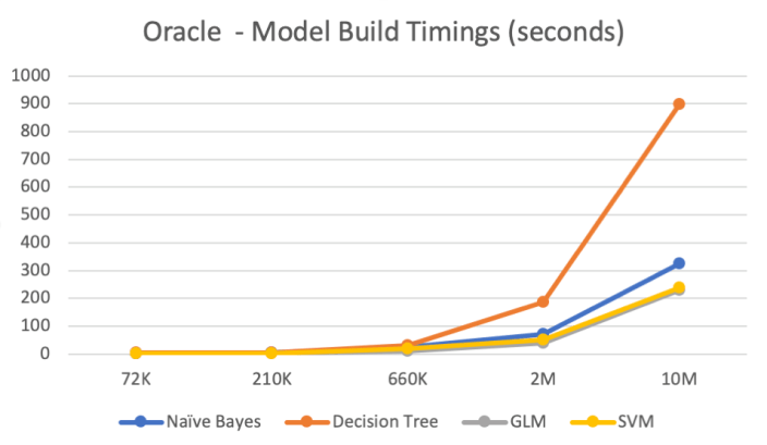
The following table below shows the length of time in seconds to build the models. All data preparations etc was done prior to this.
Note: It should be noted that Automatic Data Preparation was turned on for these algorithms. This performed additional algorithm specific data preparation for each model. That means the times given in the following tables is for some data preparation time and for building the models.
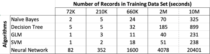
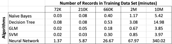
Converting the above table into minutes.
Renaming & Commenting Oracle Data Mining Models
As your company evolves with their data mining projects, the number of models produced and in use in production will increase dramatically.
Care needs to be taken when it comes to managing these. This includes using meaningful names, adding descriptions of what the model is about or for, and being able to track their usage, etc.
I will look at tracking the usage of the models in another blog post, but the following gives examples of how to rename Oracle Data Mining models and how to add comments or descriptions to these models. This is particularly useful because our data analytics teams have a constant turn over or it has been many months since you last worked on a model and you want a quick idea of what purpose of the model was for.
If you have been using the Oracle Data Mining tool (part of SQL Developer) will will see your model being created with some sort of sequencing numbers. For example for a Support Vector Machine (SVM) model you might see it labelled for classification:
CLAS_SVM_5_22
While you are working on this project you will know and understand what it was about and why it is being used. But afterward you may forget as you will be dealing with many hundreds of models. Yes you could check your documentation for the purpose of this model but that can take some time.
What if you could run a SQL query to find out?
But first we need to rename the model.
DBMS_DATA_MINING.RENAME_MODEL('CLAS_SVM_5_22', 'HIGH_VALUE_CHURN_CLAS_SVM');
Next we will want to add a longer description of what the model is about. We can do this by adding a comment to the model.
COMMENT ON MINING MODEL high_value_churn_clas_svm IS
'Classification Model to Predict High Value Customers most likely to Churn';
We can now see these updated details when we query the Oracle Data Mining models in a user schema.
SELECT model_name, mining_function, algorithm, comments
FROM user_mining_models;
These are two very useful commands.
Evaluating Cluster Dispersion in Oracle Data Mining
When working with the Clustering algorithms, and particularly k-Means, in the Oracle Data Miner tool there is no way of seeing how compact or dispersed the data is within a cluster.
There are a number of measures typically used in various tools and algorithms, but with Oracle Data Miner we are not presented with any of this information.
But if we flip from using the Oracle Data Miner tool to using SQL we can get to see some more details of the clusters produced by the k-Means algorithm along with some additional and useful information.
As I said there are a number of different measures used to evaluate clusters. The one that Oracle uses is called Dispersion. Now there are a few different definitions of what this could be and I haven’t been able to locate what is Oracle’s own definition of it in any of the documentation.
We can use the Dispersion value as a measure of how compact or how spread out the data is within a cluster. The Dispersion value is a number greater than 0. The lower the value of the more compact the cluster is i.e. the data points are close the the centroid of the cluster. The larger the value the more disperse or spread out the data points are.
The DBMS_DATA_MINING PL/SQL package comes with a function called GET_MODEL_DETAILS_KM. This function returns a record of the form DM_CLUSTERS.
(id                   NUMBER,
 cluster_id           VARCHAR2(4000),
 record_count         NUMBER,
 parent               NUMBER,
 tree_level           NUMBER,
 dispersion           NUMBER,
 split_predicate      DM_PREDICATES,
 child                DM_CHILDREN,
 centroid             DM_CENTROIDS,
 histogram            DM_HISTOGRAMS,
 rule                 DM_RULE)
We can not use the following query to get the Dispersion value for each of the clusters from an ODM cluster model.
SELECT cluster_id,
       record_count,
       parent,
       tree_level,
       dispersion
FROM  table(dbms_data_mining.get_model_details_km('CLUS_KM_3_2'));

Using the Identity column for Oracle Data Miner
If you are a user of the Oracle Data Miner tool (the workflow data mining tool that is part of SQL Developer), then you will have noticed that for many of the algorithms you can specify a Case Id attribute along with, say, the target attribute.

The idea is that you have one attribute that is a unique identifier for each case record. This may or may not be the case in your data model and you may have a multiple attribute primary key or case record identifier.
But what is the Case Id field used for in Oracle Data Miner?
Based on the documentation this field does not need to have a value. But it is recommended that you do identify an attribute for the Case Id, as this will allow for reproducible results. What this means is that if we run our workflow today and again in a few days time, on the exact same data, we should get the same results. So the Case Id allows this to happen. But how? Well it looks like the attribute used or specified for the Case Id is used as part of the Hashing algorithm to partition the data into a train and test data set, for classification problems.
So if you don’t have a single attribute case identifier in your data set, then you need to create one. There are a few options open to you to do this.
- Create one: write some code that will generate a unique identifier for each of your case records based on some defined rule.
- Use a sequence: and update the records to use this sequence.
- Use ROWID: use the unique row identifier value. You can write some code to populate this value into an attribute. Or create a view on the table containing the case records and add a new attribute that will use the ROWID. But if you move the data, then the next time you use the view then you will be getting different ROWIDs and that in turn will mean we may have different case records going into our test and training data sets. So our workflows will generate different results. Not what we want.
- Use ROWNUM: This is kind of like using the ROWID. Again we can have a view that will select ROWNUM for each record. Again we may have the same issues but if we have our data ordered in a way that ensures we get the records returned in the same order then this approach is OK to use.
- Use Identity Column: In Oracle 12c we have a new feature called Identify Column. This kind of acts like a sequence but we can defined an attribute in a table to be an Identity Column, and as records are inserted into the the data (in our scenario our case table) then this column will automatically generate a unique number for our data. Again if we need to repopulate the case table, you will need to drop and recreate the table to get the Identity Column to reset, otherwise the newly inserted records will start with the next number of the Identity Column
Here is an example of using the Identity Column in a case table.
CREATE TABLE case_table (
id_column	NUMBER GENERATED ALWAYS AS IDENTITY,
affinity_card 	NUMBER,
age		NUMBER,
cust_gender	VARCHAR2(5),
country_name	VARCHAR2(20)
...
);
You can now use this Identity Column as the Case Id in your Oracle Data Miner workflows.

Oracle Text, Oracle R Enterprise and Oracle Data Mining – Part 5
In this 5th blog post in my series on using the capabilities of Oracle Text, Oracle R Enterprise and Oracle Data Mining to process documents and text, I will have a look at some of the machine learning features of Oracle Text.
Oracle Text comes with a number of machine learning algorithms. These can be divided into two types. The first is called ‘Supervised Learning’ where we have two machine learning algorithms for classification type of problem. The second type is called ‘Unsupervised Learning’ where we have the ability to use clustering machine learning algorithms to look for patterns in our text documents and to find similarities between documents based on their contents.
It is this second type of document clustering that I will work through in this blog post.
When using clustering with text documents, the machine learning algorithm will look for patterns that are common between the documents. These patterns will include the words used, the frequency of the words, the position or ordering of these words, the co-occurance of words, etc. Yes this is a large an complex task and that is why we need a machine learning algorithm to help us.
With Oracle Text we only have one clustering machine learning algorithm available to use. When we move onto using the Oracle Advanced Analytics Option (Oracle Data Mining and Oracle R Enterprise) we more algorithms available to us.
With Oracle Text the clustering algorithm is called k-Means. In a way the actual algorithm is unimportant as it is the only one available to us when using Oracle Text. To use this algorithm we have the CTX_CLS.CLUSTERING procedure. This procedure takes the documents we want to compare and will then identify the clusters (using hierarchical clustering) and will then tells us, for each document, what clusters the documents belong to and they probability value. With clustering a document (or a record) can belong to many clusters. Typically in the text books we see clusters that are very distinct and are clearly separated from each other. When you work on real data this is never the case. We will have many over lapping clusters and a data point/record can belong to one or more clusters. This is why we need the probability vale. We can use this to determine what cluster our record belongs to most and what other clusters it is associated with.
Using the example documents that I have been using during this series of blog posts we can use the CTX_CLS.CLUSTERING algorithm to cluster and identify similarities in these documents.
We need to setup the parameters that will be used by the CTX_CLS.CLUSTERING procedure. Tell it to use the k-Means algorithm and then the number of clusters to generate. As with all Oracle Text procedures or algorithms there are a number of settings you can configure or you can just accept the default values.
exec ctx_ddl.drop_preference('Cluster_My_Documents');
exec ctx_ddl.create_preference('Cluster_My_Documents','KMEAN_CLUSTERING');
exec ctx_ddl.set_attribute('Cluster_My_Documents','CLUSTER_NUM','3');
The code above is an example of the basics of what you need to setup for clustering. Other attribute or cluster parameter setting available to you include, MAX_DOCTERMS, MAX_FEATURES, THEME_ON, TOKEN_ON, STEM_ON, MEMORY_SIZE and SECTION_WEIGHT.
Now we can run the CTX_CLS.CLUSTERING procedure on our documents. This procedure has the following parameters.
– The Oracle Text Index Name
– Document Id Column Name
– Document Assignment (cluster assignment) Table Name. This table will be created if it doesn’t already exist
– Cluster Description Table Name. This table will be created if it doesn’t already exist.
– Name of the Oracle Text Preference (list)
exec ctx_cls.clustering(
'MY_DOCUMENTS_OT_IDX',
'DOC_PK',
'OT_CLUSTER_RESULTS',
'DOC_CLUSTER_DETAILS',
'Cluster_My_Documents');
When the procedure has completed we can now examine the OT_CLUSTER_RESULTS and the DOC_CLUSTER_DETAILS tables. The first of these (OT_CLUSTER_RESULTS) allows us to see what documents have been clustered together. The following is what was produced for my documents.
SELECT d.doc_pk,
       d.doc_title,
       r.clusterid,
       r.score
FROM my_documents d,
     ot_cluster_results r
WHERE d.doc_pk = r.docid;

We can see that two of the documents have been grouped into the same cluster (ClusterId=2). If you have a look back at what these documents are about then you can see that yes these are very similar. For the other two documents we can see that they have been clustered into separate clusters (ClusterId=4 & 5). The clustering algorithms have said that they are different types of documents. Again when you examine these documents you will see that they are talking about different topics. So the clustering process worked !
You can also explore the various features of the clusters by looking that he DOC_CLUSTER_DETAILS table. Although the details in this table are not overly useful but it will give you some insight into what clusters the k-Means algorithm has produced.
Hopefully I’ve shown you how easy it is to setup and use the clustering feature of Oracle Text.
WARNING: Before using the Clustering or Classification with Oracle Text, you need to check with your local Oracle Sales representative about if there is licence implication. There seems to be some mentions the the algorithms used are those that come with Oracle Data Mining. Oracle Data Mining is a licence cost option for the database. So make sure you check before you go using these features.
Oracle Text, Oracle R Enterprise and Oracle Data Mining – Part 1
A project that I’ve been working on for a while now involves the use of Oracle Text, Oracle R Enterprise and Oracle Data Mining. Oracle Text comes with your Oracle Database licence. Oracle R Enterprise and Oracle Data Mining are part of the Oracle Advanced Analytics (extra cost) option.
What I will be doing over the course of 4 or maybe 5 blog posts is how these products can work together to help you gain a grater insight into your data, and part of your data being large text items like free format text, documents (in various forms e.g. html, xml, pdf, ms word), etc.
Unfortunately I cannot show you examples from the actual project I’ve been working on (and still am, from time to time). But what I can do is to show you how products and components can work together.
In this blog post I will just do some data setup. As with all project scenarios there can be many ways of performing the same tasks. Some might be better than others. But what I will be showing you is for demonstration purposes.
The scenario: The scenario for this blog post is that I want to extract text from some webpages and store them in a table in my schema. I then want to use Oracle Text to search the text from these webpages.
Schema setup: We need to create a table that will store the text from the webpages. We also want to create an Oracle Text index so that this text is searchable.
drop sequence my_doc_seq;
create sequence my_doc_seq;

drop table my_documents;

create table my_documents (
doc_pk number(10) primary key,
doc_title varchar2(100),
doc_extracted date,
data_source varchar2(200),
doc_text clob);

create index my_documents_ot_idx on my_documents(doc_text)
indextype is CTXSYS.CONTEXT;
In the table we have a number of descriptive attributes and then a club for storing the website text. We will only be storing the website text and not the html document (More on that later). In order to make the website text searchable in the DOC_TEXT attribute we need to create an Oracle Text index of type CONTEXT.
There are a few challenges with using this type of index. For example when you insert a new record or update the DOC_TEXT attribute, the new values/text will not be reflected instantly, just like we are use to with traditional indexes. Instead you have to decide when you want to index to be updated. For example, if you would like the index to be updated after each commit then you can create the index using the following.
create index my_documents_ot_idx on my_documents(doc_text)
indextype is CTXSYS.CONTEXT
parameters ('sync (on commit)');
Depending on the number of documents you have being committed to the DB, this might not be for you. You need to find the balance. Alternatively you could schedule the index to be updated by passing an interval to the ‘sync’ in the above command. Alternatively you might want to use DBMS_JOB to schedule the update.
To manually sync (or via DBMS_JOB) the index, assuming we used the first ‘create index’ statement, we would need to run the following.
EXEC CTX_DDL.SYNC_INDEX('my_documents_ot_idx');
This function just adds the new documents to the index. This can, over time, lead to some fragmentation of the index, and will require it to the re-organised on a semi-regular basis. Perhaps you can schedule this to happen every night, or once a week, or whatever makes sense to you.
BEGIN
  CTX_DDL.OPTIMIZE_INDEX('my_documents_ot_idx','FULL');
END;
(I could talk a lot more about setting up some basics of Oracle Text, the indexes, etc. But I’ll leave that for another day or you can read some of the many blog posts that already exist on the topic.)
Extracting text from a webpage using R: Some time ago I wrote a blog post on using some of the text mining features and packages in R to produce a word cloud based on some of the Oracle Advanced Analytics webpages.
I’m going to use the same webpages and some of the same code/functions/packages here.
The first task you need to do is to get your hands on the ‘htmlToText function. You can download the htmlToText function on github. This function requires the ‘Curl’ and ‘XML’ R packages. So you may need to install these.
I also use the str_replace_all function (“stringer’ R package) to remove some of the html that remains, to remove some special quotes and to replace and occurrences of ‘&’ with ‘and’.
# Load the function and required R packages
source(“c:/app/htmltotext.R”)
library(stringr)
data1 <- str_replace_all(htmlToText("http://www.oracle.com/technetwork/database/options/advanced-analytics/overview/index.html"), "[\r\n\t\"\'\u201C\u201D]" , "")
data1 <- str_replace_all(data1, "&", "and")
data2 <- str_replace_all(str_replace_all(htmlToText("http://www.oracle.com/technetwork/database/options/advanced-analytics/odm/index.html"), "[\r\n\t\"\'\u201C\u201D]" , ""), "&", "and")
data2 <- str_replace_all(data2, "&", "and")
data3 <- str_replace_all(str_replace_all(htmlToText("http://www.oracle.com/technetwork/database/database-technologies/r/r-technologies/overview/index.html"), "[\r\n\t\"\'\u201C\u201D]" , ""), "&", "and")
data3 <- str_replace_all(data3, "&", "and")
data4 <- str_replace_all(str_replace_all(htmlToText("http://www.oracle.com/technetwork/database/database-technologies/r/r-enterprise/overview/index.html"), "[\r\n\t\"\'\u201C\u201D]" , ""), "&", "and")
data4 <- str_replace_all(data4, "&", "and")
We now have the text extracted and cleaned up.
Create a data frame to contain all our data: Now that we have the text extracted, we can prepare the other data items we need to insert the data into our table (‘my_documents’). The first stept is to construct a data frame to contain all the data.
data_source = c("http://www.oracle.com/technetwork/database/options/advanced-analytics/overview/index.html",
                 "http://www.oracle.com/technetwork/database/options/advanced-analytics/odm/index.html",
                 "http://www.oracle.com/technetwork/database/database-technologies/r/r-technologies/overview/index.html",
                 "http://www.oracle.com/technetwork/database/database-technologies/r/r-enterprise/overview/index.html")
doc_title = c("OAA_OVERVIEW", "OAA_ODM", "R_TECHNOLOGIES", "OAA_ORE")
doc_extracted = Sys.Date()
data_text <- c(data1, data2, data3, data4)

my_docs <- data.frame(doc_title, doc_extracted, data_source, data_text)
Insert the data into our database table: With the data in our data fram (my_docs) we can now use this data to insert into our database table. There are a number of ways of doing this in R. What I’m going to show you here is how to do it using Oracle R Enterprise (ORE). The thing with ORE is that there is no explicit functionality for inserting and updating records in a database table. What you need to do is to construct, in my case, the insert statement and then use ore.exec to execute this statement in the database.

You must be logged in to post a comment.