
data mining
AutoML – using TPOT
Another popular AutoML library is TPOT, which stands for Tree-Based Pipeline Optimization Tool. The goal of TPOT is to automate the building of ML pipelines by combining a flexible expression tree representation of pipelines with stochastic search algorithms such as genetic programming. TPOT makes use of the Python-based scikit-learn library
Install the TPOT library using
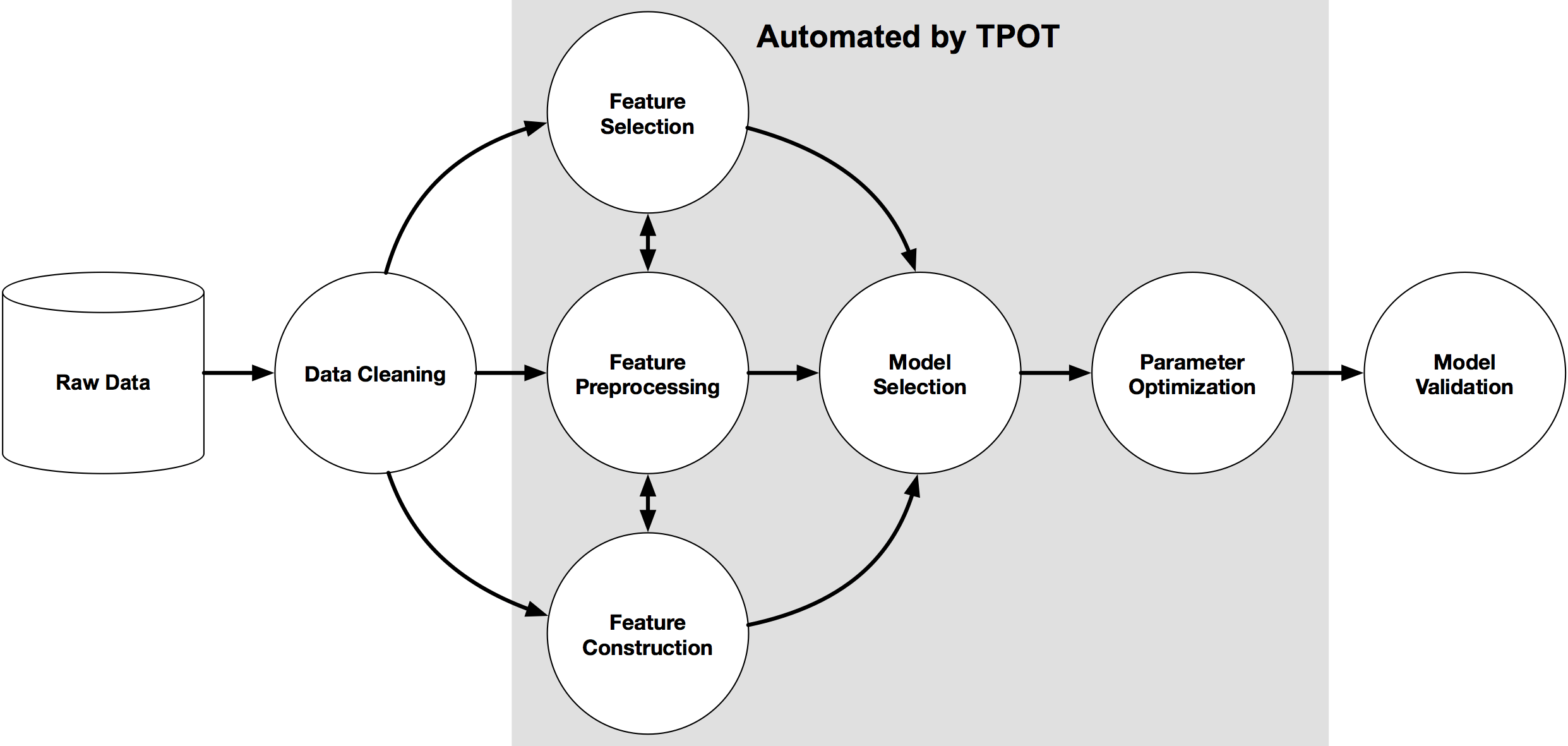
pip3 install tpotHere is an example tree-based pipeline from TPOT. Each circle corresponds to a machine learning operator, and the arrows indicate the direction of the data flow

Let’s build upon my previous blog post on AutomML, by using the same data set, with no modifications, and using the training (X_train, y_train) and test (X_test, y_test) data sets (dataframes), based on the Bank data sets. Check the previous post for the detailed steps on getting to this point.
In a similar way as the autosklean library example, I’m just going to demonstrate using TPOT for a classification problem using TPOTClassifier class. For regression problems, there is the corresponding TPOTRegressor class (not demonstrated in this post).
TPOTClassifier has the following main parameters (there are others):
- generations: Number of iterations to the run pipeline optimization process. The default is 100.
- population_size: Number of individuals to retain in the genetic programming population every generation. The default is 100.
- offspring_size: Number of offspring to produce in each genetic programming generation. The default is 100.
- mutation_rate: Mutation rate for the genetic programming algorithm in the range [0.0, 1.0]. This parameter tells the GP algorithm how many pipelines to apply random changes to every generation. Default is 0.9
- crossover_rate: Crossover rate for the genetic programming algorithm in the range [0.0, 1.0]. This parameter tells the genetic programming algorithm how many pipelines to “breed” every generation.
- scoring: Function used to evaluate the quality of a given pipeline for the classification problem like
accuracy,average_precision,roc_auc,recall, etc. The default isaccuracy. - cv: Cross-validation strategy used when evaluating pipelines. The default is 5.
- random_state: The seed of the pseudo-random number generator used in TPOT. Use this parameter to make sure that TPOT will give you the same results each time you run it against the same data set with that seed.
- verbosity: How much information TPOT communicates while it is running. Default is 0 (zero) TPOT will display nothing. 1=display minimal information, 2=display more information and progress bar, 3=print everything and progress bar.
- n_jobs: Number of processes to use. Default is 1. Use -1 to use all available cores.
Care is needed with some of these settings, for example generations should be set small to begin with, for example set to 5 initially. Also, population_size should also be kept small, for example 5 initially. These initial settings will evaluate 25 piplelines (5×5) configurations before finishing, and for some these settings may need to be adjusted smaller for initial work/investigations. Another parameter to adjust is the ‘verbosity’ setting. The default is 0 which means no details will be displayed. I like to set this to 3, as it gives more details of the outcomes from each pipeline. Adjust higher for more details or lower to fewer details. Another parameter to consider adjusting is ‘max_time_min’ and ‘max_eval_time_min’, but setting these too low can result in no or minimum results.
Load the library, setup the configuration and run. This is very simple to setup
from tpot import TPOTClassifier

#configure settings
tpot = TPOTClassifier(generations=5, population_size=5, verbosity=3, n_jobs=4, scoring='accuracy')

#run TPOT
tpot.fit(X_train, y_train)
As verbosity is set to 3 we get a lot of detail being displayed for each generation. The final output is shown below. What is missing from this is the progress bars which are displayed while TPOT is running
32 operators have been imported by TPOT.


Generation 1 - Current Pareto front scores:

-1	0.8963961891371728	RandomForestClassifier(input_matrix, RandomForestClassifier__bootstrap=True, RandomForestClassifier__criterion=gini, RandomForestClassifier__max_features=0.7000000000000001, RandomForestClassifier__min_samples_leaf=5, RandomForestClassifier__min_samples_split=7, RandomForestClassifier__n_estimators=100)

-2	0.8978183008194085	RandomForestClassifier(ZeroCount(input_matrix), RandomForestClassifier__bootstrap=True, RandomForestClassifier__criterion=gini, RandomForestClassifier__max_features=0.7000000000000001, RandomForestClassifier__min_samples_leaf=5, RandomForestClassifier__min_samples_split=7, RandomForestClassifier__n_estimators=100)
Pipeline encountered that has previously been evaluated during the optimization process. Using the score from the previous evaluation.

Generation 2 - Current Pareto front scores:

-1	0.8974020496851336	RandomForestClassifier(input_matrix, RandomForestClassifier__bootstrap=True, RandomForestClassifier__criterion=gini, RandomForestClassifier__max_features=0.7000000000000001, RandomForestClassifier__min_samples_leaf=8, RandomForestClassifier__min_samples_split=7, RandomForestClassifier__n_estimators=100)

-2	0.8978183008194085	RandomForestClassifier(ZeroCount(input_matrix), RandomForestClassifier__bootstrap=True, RandomForestClassifier__criterion=gini, RandomForestClassifier__max_features=0.7000000000000001, RandomForestClassifier__min_samples_leaf=5, RandomForestClassifier__min_samples_split=7, RandomForestClassifier__n_estimators=100)
_pre_test decorator: _random_mutation_operator: num_test=0 '(slice(None, None, None), 0)' is an invalid key.
Pipeline encountered that has previously been evaluated during the optimization process. Using the score from the previous evaluation.

Generation 3 - Current Pareto front scores:

-1	0.8974020496851336	RandomForestClassifier(input_matrix, RandomForestClassifier__bootstrap=True, RandomForestClassifier__criterion=gini, RandomForestClassifier__max_features=0.7000000000000001, RandomForestClassifier__min_samples_leaf=8, RandomForestClassifier__min_samples_split=7, RandomForestClassifier__n_estimators=100)

-2	0.8978183008194085	RandomForestClassifier(ZeroCount(input_matrix), RandomForestClassifier__bootstrap=True, RandomForestClassifier__criterion=gini, RandomForestClassifier__max_features=0.7000000000000001, RandomForestClassifier__min_samples_leaf=5, RandomForestClassifier__min_samples_split=7, RandomForestClassifier__n_estimators=100)
Skipped pipeline #21 due to time out. Continuing to the next pipeline.
Skipped pipeline #23 due to time out. Continuing to the next pipeline.

Generation 4 - Current Pareto front scores:

-1	0.8974020496851336	RandomForestClassifier(input_matrix, RandomForestClassifier__bootstrap=True, RandomForestClassifier__criterion=gini, RandomForestClassifier__max_features=0.7000000000000001, RandomForestClassifier__min_samples_leaf=8, RandomForestClassifier__min_samples_split=7, RandomForestClassifier__n_estimators=100)

-2	0.8978183008194085	RandomForestClassifier(ZeroCount(input_matrix), RandomForestClassifier__bootstrap=True, RandomForestClassifier__criterion=gini, RandomForestClassifier__max_features=0.7000000000000001, RandomForestClassifier__min_samples_leaf=5, RandomForestClassifier__min_samples_split=7, RandomForestClassifier__n_estimators=100)

Generation 5 - Current Pareto front scores:

-1	0.8983385200075953	RandomForestClassifier(input_matrix, RandomForestClassifier__bootstrap=True, RandomForestClassifier__criterion=gini, RandomForestClassifier__max_features=0.55, RandomForestClassifier__min_samples_leaf=8, RandomForestClassifier__min_samples_split=7, RandomForestClassifier__n_estimators=100)

TPOTClassifier(generations=5, n_jobs=4, population_size=5, scoring='accuracy',
               verbosity=3)
We can now display the ‘best’ model configuration discovered by TPOT.
tpot.fitted_pipeline_


Pipeline(steps=[('normalizer', Normalizer(norm='l1')),
                ('xgbclassifier',
                 XGBClassifier(base_score=0.5, booster='gbtree',
                               colsample_bylevel=1, colsample_bynode=1,
                               colsample_bytree=1, gamma=0, gpu_id=-1,
                               importance_type='gain',
                               interaction_constraints='', learning_rate=0.01,
                               max_delta_step=0, max_depth=8,
                               min_child_weight=7, missing=nan,
                               monotone_constraints='()', n_estimators=100,
                               n_jobs=1, num_parallel_tree=1, random_state=0,
                               reg_alpha=0, reg_lambda=1, scale_pos_weight=1,
                               subsample=0.8, tree_method='exact',
                               validate_parameters=1, verbosity=0))])
In this run of TPOT, on this data set, XGBoost algorithm gave the best results using the parameters and settings listed above. What is interesting, everytime I’ve run TPOT for the same data set, using the same configuration parameters, I get a slightly different outcome.
Next step is to evaluate the ‘best’ model on the holdout data set.
tpot.score(X_test, y_test)


0.9037792344420167
The results achieved are good and are better than some of the other models created by other AutoML libraries.
The final step we can perform is to export the model template. This creates a file containing the template code to create and use the model. This does require some modifications to specify the data set, and the pipeline of data modifications and transformations.
#export the model
tpot.export('.../tpot_Bank_pipeline.py')
The output file contains the following.
import numpy as np
import pandas as pd
from sklearn.model_selection import train_test_split
from sklearn.pipeline import make_pipeline
from sklearn.preprocessing import Normalizer
from xgboost import XGBClassifier

# NOTE: Make sure that the outcome column is labeled 'target' in the data file
tpot_data = pd.read_csv('PATH/TO/DATA/FILE', sep='COLUMN_SEPARATOR', dtype=np.float64)
features = tpot_data.drop('target', axis=1)

training_features, testing_features, training_target, testing_target = \
            train_test_split(features, tpot_data['target'], random_state=None)

# Average CV score on the training set was: 0.8986507248984001
exported_pipeline = make_pipeline(
    Normalizer(norm="l1"),
    XGBClassifier(learning_rate=0.01, max_depth=8, min_child_weight=7, n_estimators=100, n_jobs=1, subsample=0.8, verbosity=0)
)

exported_pipeline.fit(training_features, training_target)
results = exported_pipeline.predict(testing_features)
TPOT does have some issues and limitations. Well it is slow, and part of this is due to the nature of genetic algorithms, every time you run TPOT you may get different results, etc. Some of these issues can be addressed by adjusting some of the parameters, but even still, it doesn’t eliminate all of them. Running on GPU helps a little with timing of each run. TPOT doesn’t remove the need for data cleaning, feature engineering etc, but that is the case with most solutions.
AutoML, what is it good for? It Depends!
Automated Machine Learning (AutoML) seems to be everywhere and every Analytics product and SaaS offering seems to have some element of AutoML built into them. Part of the reason for this is because most of the market analysts, such as Gartner etc., have been rating Machine Learning (ML) products and services based on them having an AutoML feature.

Some of the benefits of AutoML is it will automatically generate a ML model for you without you having to worry about any of the technical details and the various statistical tests to measure if the model is useful. This kind of message has resulted is lots and lots of articles talking about the death of the Data Scientist, as they are no longer needed. We must remember ML is only one of the tools and skills of the data scientist.
This can all sound great. No need to hire these expensive data scientists, I can just use this AutoML software to create a ML model, for my data, and life will be good with all these wonderful predictions. Just think of the money I’ll be making and saving!
Where the fun comes into all of this is when someone issues legal proceedings based on what one of these AutoML models has predicted. The AutoML has made an incorrect prediction. The problem you now face, probably in court, is trying to justify the prediction by saying the machine/computer/algorithm made it, and you have no idea how or what it is doing to make the prediction. Good luck in a court explaining that to a judge and/or jury. Be prepared to hand over lots of money
What is missing is the human in the loop, and in most cases this will be the data scientist or machine learning engineer (or someone else with a really cool job title). Part of their job is to evaluate lots of difference models for you data (remember they will create lots and lots of models and not just one!), determine (from experimentation) what algorithms work best with your data and problem, optimize these models and assess the impact of changing hyperparameters, look at how these ML models are behaving, are there any biases in the model or data, use a wide variety of statistic tests to assess the models, examine how the model works with different sub-parts of the data (customers), look at any potential legal and legislative issues not just in one geographic but across many disparate regions all of which have different legal requirements, etc.
As you can see there are many additional tasks beyond the ML steps needed to create, verify and select a ML to use. All of this is before you look at how it can be deployed in your production systems/architecture and building out you MLOps.
One importing characteristic of having the human in the loop is Explainability. Explainability of the process followed, what models were produced, the effect of tuning and opimizing, possible biases and mitigating steps, etc etc The list goes on and on. This the role of the data scientist and now it might look like a good idea to hire a good data scientist who understands all of this.

Taking a little step back, AutoML is kind of good cool feature/tool. A lot of the main steps of creating all those ML models, tuning them and evaluating them, etc can be very boring work. You do same steps for each model and do it all over again for the next, and so on for the tens or hundreds of models you will be creating. Most data scientists will have scripts in their toolbox (based from their experience) to automatically perform all of these steps and output the results. I mentioned the word experience in the last sentence. It can take a bit of time to build up to this. The AutoML products will do all of this automatically for you hence you don’t have to hire a data scientist to do it (see what I said above about this).
I mentioned above some of the challenges and the need to keep a human in the loop. AutoML can be seen as another tool to assist the data scientist and not to replace them. AutoML can be used to to help the data scientist work towards identifying what ML models to use. But this can be a bit of a challenge to do. It depends on what product or library you use. Some AutoML solutions act as a black box. Kind of like the image at the top of this post. These are simple to use but the draw back is there is not explainability or ability of the data scientist to really assess what is happening at each step. There are AutoML products/solutions that allow you to inspect and monitor what is happening at each step within AutoML. The diagram given able is one example of this. This allows for the human in the loop and allows for explainability. If the data scientist sees some unusual direction being taken by AutoML they can see where and why this is happening and can take corrective action. AutoML isn’t a black box in this scenario.
I mentioned above, AutoML can be another tool for the data scientist to use. Look on AutoML as quick way to see what might be possible. Using the information from each step of AutoML, the data scientist can use this information to guide them towards creating a more suitable and usable ML model, and do so in perhaps a slightly shorter space of time.
Going back to the title of the post ‘AutoML, what is it good for?’, the answer really is ‘It Depends!’, but if you do use it, be careful how you use the models and results beyond doing some simple investigation. And be careful of product offerings saying you don’t need anything else.
Adding Text Processing to Classification Machine Learning in Oracle Machine Learning
One of the typical machine learning functions is Classification. This is in widespread use across most domains and geographic regions. I’ve written several blog posts on this topic over many years (and going back many, many year) on how to do this using Oracle Machine Learning (OML) (formally known as Oracle Advanced Analytic and in the Oracle Data Miner tool in SQL Developer). Just do a quick search of my blog to find some of these posts.
When it comes to Classification problems, typically the data set will be contain your typical categorical and numerical variables/features. The Automatic Data Preparation (ADP) feature of OML where it automatically pre-processes and transforms these variable for input to the machine learning algorithm. This greatly reduces the boring work of the data scientist and increases their productivity.
But sometimes data sets come with text descriptions. These will contain production descriptions, free format text, and other descriptive data, for example product reviews. But how can this information be included as part of the input data set to the machine learning algorithms. Oracle allows this kind of input data, and a letting bit of setup is needed to tell Oracle how to process the data set. This uses the in-database feature of Oracle Text.
The following example walks through an example of the steps needed to pre-process and include the text processing as part of the machine learning algorithm.
The data set: The data used to illustrate this and to show the steps needed, is a data set from Kaggle webiste. This data set contains 130K Wine Reviews. This data set contain descriptive information of the wine with attributes about each wine including country, region, number of points, price, etc as well as a text description contain a review of the wine.
The following are 2 files containing the DDL (to create the table) and then Import the data set (using sql script with insert statements). These can be run in your schema (in order listed below).
I’ll leave the Data Exploration to you to do and to discover some early insights.
The ML Question
I want to be able to predict if a wine is a good quality wine, based on the prices and different characteristics of the wine?
Data Preparation
To be able to answer this question the first thing needed is to define a target variable to identify good and bad wines. To do this create a new attribute/feature called POINTS_BIN and populate it based on the number of points a wine has. If it has >90 points it is a good wine, if <90 points it is a bad wine.
ALTER TABLE WineReviews130K_bin ADD POINTS_BIN VARCHAR2(15);

UPDATE WineReviews130K_bin
SET POINTS_BIN = 'GT_90_Points'
WHERE winereviews130k_bin.POINTS >= 90;

UPDATE WineReviews130K_bin
SET POINTS_BIN = 'LT_90_Points'
WHERE winereviews130k_bin.POINTS < 90;

alter table WineReviews130K_bin DROP COLUMN POINTS;
The DESCRIPTION column data type needs to be changed to CLOB. This is to allow the Text Mining feature to work correctly.
-- add a new column of data type CLOB
ALTER TABLE WineReviews130K_bin ADD (DESCRIPTION_NEW CLOB);

-- update new column with data from the DESCRIPTION attribute
UPDATE WineReviews130K_bin SET DESCRIPTION_NEW = DESCRIPTION;

-- drop the DESCRIPTION attribute from table
ALTER TABLE WineReviews130K_bin DROP COLUMN DESCRIPTION;

-- rename the new attribute to replace DESCRIPTION
ALTER TABLE WineReviews130K_bin RENAME COLUMN DESCRIPTION_NEW TO DESCRIPTION;
Text Mining Configuration
There are a number of things we need to define for the Text Mining to work, these include a Lexer, Stop Word list and preferences.
First define the Lexer to use. In this case we will use a basic one and basic settings
BEGIN
   ctx_ddl.create_preference('mylex', 'BASIC_LEXER');
   ctx_ddl.set_attribute('mylex', 'printjoins', '_-');
   ctx_ddl.set_attribute ( 'mylex', 'index_themes', 'NO');
   ctx_ddl.set_attribute ( 'mylex', 'index_text', 'YES');
END;
Next we can define a Stop Word List. Oracle Text comes with a predefined set of Stop Word lists for most of the common languages. You can add to one of those list or create your own. Depending on the domain you are working in it might be easier to create your own and it is very straight forward to do. For example:
DECLARE
   v_stoplist_name varchar2(100);
BEGIN
   v_stoplist_name := 'mystop';
   ctx_ddl.create_stoplist(v_stoplist_name, 'BASIC_STOPLIST');
   ctx_ddl.add_stopword(v_stoplist_name, 'nonetheless');
   ctx_ddl.add_stopword(v_stoplist_name, 'Mr');
   ctx_ddl.add_stopword(v_stoplist_name, 'Mrs');
   ctx_ddl.add_stopword(v_stoplist_name, 'Ms');
   ctx_ddl.add_stopword(v_stoplist_name, 'a');
   ctx_ddl.add_stopword(v_stoplist_name, 'all');
   ctx_ddl.add_stopword(v_stoplist_name, 'almost');
   ctx_ddl.add_stopword(v_stoplist_name, 'also');
   ctx_ddl.add_stopword(v_stoplist_name, 'although');
   ctx_ddl.add_stopword(v_stoplist_name, 'an');
   ctx_ddl.add_stopword(v_stoplist_name, 'and');
   ctx_ddl.add_stopword(v_stoplist_name, 'any');
   ctx_ddl.add_stopword(v_stoplist_name, 'are');
   ctx_ddl.add_stopword(v_stoplist_name, 'as');
   ctx_ddl.add_stopword(v_stoplist_name, 'at');
   ctx_ddl.add_stopword(v_stoplist_name, 'be');
   ctx_ddl.add_stopword(v_stoplist_name, 'because');
   ctx_ddl.add_stopword(v_stoplist_name, 'been');
   ctx_ddl.add_stopword(v_stoplist_name, 'both');
   ctx_ddl.add_stopword(v_stoplist_name, 'but');
   ctx_ddl.add_stopword(v_stoplist_name, 'by');
   ctx_ddl.add_stopword(v_stoplist_name, 'can');
   ctx_ddl.add_stopword(v_stoplist_name, 'could');
   ctx_ddl.add_stopword(v_stoplist_name, 'd');
   ctx_ddl.add_stopword(v_stoplist_name, 'did');
   ctx_ddl.add_stopword(v_stoplist_name, 'do');
   ctx_ddl.add_stopword(v_stoplist_name, 'does');
   ctx_ddl.add_stopword(v_stoplist_name, 'either');
   ctx_ddl.add_stopword(v_stoplist_name, 'for');
   ctx_ddl.add_stopword(v_stoplist_name, 'from');
   ctx_ddl.add_stopword(v_stoplist_name, 'had');
   ctx_ddl.add_stopword(v_stoplist_name, 'has');
   ctx_ddl.add_stopword(v_stoplist_name, 'have');
   ctx_ddl.add_stopword(v_stoplist_name, 'having');
   ctx_ddl.add_stopword(v_stoplist_name, 'he');
   ctx_ddl.add_stopword(v_stoplist_name, 'her');
   ctx_ddl.add_stopword(v_stoplist_name, 'here');
   ctx_ddl.add_stopword(v_stoplist_name, 'hers');
   ctx_ddl.add_stopword(v_stoplist_name, 'him');
   ctx_ddl.add_stopword(v_stoplist_name, 'his');
   ctx_ddl.add_stopword(v_stoplist_name, 'how');
   ctx_ddl.add_stopword(v_stoplist_name, 'however');
   ctx_ddl.add_stopword(v_stoplist_name, 'i');
   ctx_ddl.add_stopword(v_stoplist_name, 'if');
   ctx_ddl.add_stopword(v_stoplist_name, 'in');
   ctx_ddl.add_stopword(v_stoplist_name, 'into');
   ctx_ddl.add_stopword(v_stoplist_name, 'is');
   ctx_ddl.add_stopword(v_stoplist_name, 'it');
   ctx_ddl.add_stopword(v_stoplist_name, 'its');
   ctx_ddl.add_stopword(v_stoplist_name, 'just');
   ctx_ddl.add_stopword(v_stoplist_name, 'll');
   ctx_ddl.add_stopword(v_stoplist_name, 'me');
   ctx_ddl.add_stopword(v_stoplist_name, 'might');
   ctx_ddl.add_stopword(v_stoplist_name, 'my');
   ctx_ddl.add_stopword(v_stoplist_name, 'no');
   ctx_ddl.add_stopword(v_stoplist_name, 'non');
   ctx_ddl.add_stopword(v_stoplist_name, 'nor');
   ctx_ddl.add_stopword(v_stoplist_name, 'not');
   ctx_ddl.add_stopword(v_stoplist_name, 'of');
   ctx_ddl.add_stopword(v_stoplist_name, 'on');
   ctx_ddl.add_stopword(v_stoplist_name, 'one');
   ctx_ddl.add_stopword(v_stoplist_name, 'only');
   ctx_ddl.add_stopword(v_stoplist_name, 'onto');
   ctx_ddl.add_stopword(v_stoplist_name, 'or');
   ctx_ddl.add_stopword(v_stoplist_name, 'our');
   ctx_ddl.add_stopword(v_stoplist_name, 'ours');
   ctx_ddl.add_stopword(v_stoplist_name, 's');
   ctx_ddl.add_stopword(v_stoplist_name, 'shall');
   ctx_ddl.add_stopword(v_stoplist_name, 'she');
   ctx_ddl.add_stopword(v_stoplist_name, 'should');
   ctx_ddl.add_stopword(v_stoplist_name, 'since');
   ctx_ddl.add_stopword(v_stoplist_name, 'so');
   ctx_ddl.add_stopword(v_stoplist_name, 'some');
   ctx_ddl.add_stopword(v_stoplist_name, 'still');
   ctx_ddl.add_stopword(v_stoplist_name, 'such');
   ctx_ddl.add_stopword(v_stoplist_name, 't');
   ctx_ddl.add_stopword(v_stoplist_name, 'than');
   ctx_ddl.add_stopword(v_stoplist_name, 'that');
   ctx_ddl.add_stopword(v_stoplist_name, 'the');
   ctx_ddl.add_stopword(v_stoplist_name, 'their');
   ctx_ddl.add_stopword(v_stoplist_name, 'them');
   ctx_ddl.add_stopword(v_stoplist_name, 'then');
   ctx_ddl.add_stopword(v_stoplist_name, 'there');
   ctx_ddl.add_stopword(v_stoplist_name, 'therefore');
   ctx_ddl.add_stopword(v_stoplist_name, 'these');
   ctx_ddl.add_stopword(v_stoplist_name, 'they');
   ctx_ddl.add_stopword(v_stoplist_name, 'this');
   ctx_ddl.add_stopword(v_stoplist_name, 'those');
   ctx_ddl.add_stopword(v_stoplist_name, 'though');
   ctx_ddl.add_stopword(v_stoplist_name, 'through');
   ctx_ddl.add_stopword(v_stoplist_name, 'thus');
   ctx_ddl.add_stopword(v_stoplist_name, 'to');
   ctx_ddl.add_stopword(v_stoplist_name, 'too');
   ctx_ddl.add_stopword(v_stoplist_name, 'until');
   ctx_ddl.add_stopword(v_stoplist_name, 've');
   ctx_ddl.add_stopword(v_stoplist_name, 'very');
   ctx_ddl.add_stopword(v_stoplist_name, 'was');
   ctx_ddl.add_stopword(v_stoplist_name, 'we');
   ctx_ddl.add_stopword(v_stoplist_name, 'were');
   ctx_ddl.add_stopword(v_stoplist_name, 'what');
   ctx_ddl.add_stopword(v_stoplist_name, 'when');
   ctx_ddl.add_stopword(v_stoplist_name, 'where');
   ctx_ddl.add_stopword(v_stoplist_name, 'whether');
   ctx_ddl.add_stopword(v_stoplist_name, 'which');
   ctx_ddl.add_stopword(v_stoplist_name, 'while');
   ctx_ddl.add_stopword(v_stoplist_name, 'who');
   ctx_ddl.add_stopword(v_stoplist_name, 'whose');
   ctx_ddl.add_stopword(v_stoplist_name, 'why');
   ctx_ddl.add_stopword(v_stoplist_name, 'will');
   ctx_ddl.add_stopword(v_stoplist_name, 'with');
   ctx_ddl.add_stopword(v_stoplist_name, 'would');
   ctx_ddl.add_stopword(v_stoplist_name, 'yet');
   ctx_ddl.add_stopword(v_stoplist_name, 'you');
   ctx_ddl.add_stopword(v_stoplist_name, 'your');
   ctx_ddl.add_stopword(v_stoplist_name, 'yours');
   ctx_ddl.add_stopword(v_stoplist_name, 'drink');
   ctx_ddl.add_stopword(v_stoplist_name, 'flavors');
   ctx_ddl.add_stopword(v_stoplist_name, '2020');
   ctx_ddl.add_stopword(v_stoplist_name, 'now');
END;
Next define the preferences for processing the Text, for example what Stop Word list to use, if Fuzzy match is to be used and what language to use for this, number of tokens/words to process and if stemming is to be used.
BEGIN
   ctx_ddl.create_preference('mywordlist', 'BASIC_WORDLIST');
   ctx_ddl.set_attribute('mywordlist','FUZZY_MATCH','ENGLISH');
   ctx_ddl.set_attribute('mywordlist','FUZZY_SCORE','1');
   ctx_ddl.set_attribute('mywordlist','FUZZY_NUMRESULTS','5000');
   ctx_ddl.set_attribute('mywordlist','SUBSTRING_INDEX','TRUE');
   ctx_ddl.set_attribute('mywordlist','STEMMER','ENGLISH');
END;
And the final step is to piece it all together by defining a new Text policy
BEGIN
   ctx_ddl.create_policy('my_policy', NULL, NULL, 'mylex', 'mystop', 'mywordlist');
END;
Define Settings for OML Model
We will create two models. An Attribute Importance model and a Classification model. The following defines the model parameters for each of these.
CREATE TABLE att_import_model_settings (setting_name varchar2(30), setting_value varchar2(30));
INSERT INTO att_import_model_settings (setting_name, setting_value)
VALUES (''ALGO_NAME'', ''ALGO_AI_MDL'');
INSERT INTO att_import_model_settings (setting_name, setting_value)
VALUES (''PREP_AUTO'', ''ON'');
INSERT INTO att_import_model_settings (setting_name, setting_value)
VALUES (''ODMS_TEXT_POLICY_NAME'', ''my_policy'');
INSERT INTO att_import_model_settings (setting_name, setting_value)
VALUES (''ODMS_TEXT_MAX_FEATURES'', ''3000'')';
CREATE TABLE wine_model_settings (setting_name varchar2(30), setting_value varchar2(30));
INSERT INTO wine_model_settings (setting_name, setting_value)
VALUES (''ALGO_NAME'', ''ALGO_RANDOM_FOREST'');
INSERT INTO wine_model_settings (setting_name, setting_value)
VALUES (''PREP_AUTO'', ''ON'');
INSERT INTO wine_model_settings (setting_name, setting_value)
VALUES (''ODMS_TEXT_POLICY_NAME'', ''my_policy'');
INSERT INTO wine_model_settings (setting_name, setting_value)
VALUES (''ODMS_TEXT_MAX_FEATURES'', ''3000'')';
Create the Training and Test data sets.
CREATE TABLE wine_train_data
AS SELECT id, country, description, designation, points_bin, price, province, region_1, region_2, taster_name, variety, title
FROM winereviews130k_bin
SAMPLE (60) SEED (1);
CREATE TABLE wine_test_data
AS SELECT id, country, description, designation, points_bin, price, province, region_1, region_2, taster_name, variety, title
FROM winereviews130k_bin
WHERE id NOT IN (SELECT id FROM wine_train_data);
All the set up is done, we can move onto the creating the machine learning models.
Create the OML Model (Attribute Importance & Classification)
We are going to create two models. The first is an Attribute Important model. This will look at the data set and will determine what attributes contribute most towards determining the target variable. As we are incorporting Texting Mining we will see what words/tokens from the DESCRIPTION attribute also contribute towards the target variable.
BEGIN
   DBMS_DATA_MINING.CREATE_MODEL(
      model_name          => 'GOOD_WINE_AI',
      mining_function     => DBMS_DATA_MINING.ATTRIBUTE_IMPORTANCE,
      data_table_name     => 'winereviews130k_bin',
      case_id_column_name => 'ID',
      target_column_name  => 'POINTS_BIN',
      settings_table_name => 'att_import_mode_settings');
END;
We can query the system views for Oracle ML to find out what are the important variables.
SELECT * FROM dm$vagood_wine_ai
ORDER BY attribute_rank;
Here is the listing of the top 15 most important attributes. We can see from the first 15 rows and looking under column ATTRIBUTE_SUBNAME, the words from the DESCRIPTION attribute that seem to be important and contribute towards determining the value in the target attribute.

At this point you might determine, based on domain knowledge, some of these words should be excluded as they are generic for the domain. In this case, go back to the Stop Word List and recreate it with any additional words. This can be repeated until you are happy with the list. In this example, WINE could be excluded by including it in the Stop Word List.
Run the following to create the Classification model. It is very similar to what we ran above with minor changes to the name of the model, the data mining function and the name of the settings table.
BEGIN
   DBMS_DATA_MINING.CREATE_MODEL(
      model_name          => 'GOOD_WINE_MODEL',
      mining_function     => DBMS_DATA_MINING.CLASSIFICATION,
      data_table_name     => 'winereviews130k_bin',
      case_id_column_name => 'ID',
      target_column_name  => 'POINTS_BIN',
      settings_table_name => 'wine_model_settings');
END;
Apply OML Model
The model can be applied in similar ways to any other ML model created using OML. For example the following displays the wine details along with the predicted points bin values (good or bad) and the probability score (<=1) of the prediction.
SELECT id, price, country, designation, province, variety, points_bin,
       PREDICTION(good_wine_mode USING *) pred_points_bin,
       PREDICTION_PROBABILITY(good_wine_mode USING *) prob_points_bin
FROM wine_test_data;
Pre-build Machine Learning Models
Machine learning has seen widespread adoption over the past few years. In more recent times we have seem examples of how the models, created by the machine learning algorithms, can be shared. There have been various approaches to sharing these models using different model interchange languages. Some of these have become more or less popular over time, for example a few years ago PMML was very popular, and in more recent times ONNX seems to popular. Who knows what it will be next year or in a couple of years time.
With the increased use of machine learning models and the ability to share them, we are now seeing other uses of them. Typically the sharing of models involved a company transferring a model developed by the data scientists in their lab environment, to DevOps teams who then deploy the model into the production environment. This has developed a new are of expertise of MLOps or AIOps.
The languages and tools used by the data scientists in the lab environment are different to the languages used to deploy applications in production. The model interchange languages can be used take the model parameters, algorithm type and data transformations, etc and map these into the interchange language. The production environment would read this interchange object and apply it to the production language. In such situations the models will use the algorithms already coded in the production language. For example, the lab environment could be using Python. But the product environment could be using C, Java, Go, etc. Python is an interpretative language and in a lot of cases is not suitable for real-time use in a production environment, due to speed and scalability issues. In this case the underlying algorithm of the production language will be used and not algorithm used in the lab. In theory the algorithms should be the same. For example a decision tree algorithm using Gini Index in one language should function in the same way in another language. We all know there can be a small to a very large difference between what happens in theory and how it works in practice. Different language and different developers will do things slightly differently. This means there will be differences between the accuracy of the models developed in the lab versus the accuracy of the (same) model used in production. As long as everyone is aware of this, then everything will be ok. But it will be important task, for the data science team, to have some measurements of these differences.

Moving on a little this a little, we are now seeing some other developments with the development and sharing of machine learning models, and the use of these open model interchange languages, like ONNX, makes this possible.
We are now seeing people making their machine learning models available to the wider community, instead of keeping them within their own team or organization.
Why would some one do this? why would they share their machine learning model? It’s a bit like the picture to the left which comes from a very popular kids programme on the BBC called Blue Peter. They would regularly show some craft projects for kids to work on at home. They would never show all the steps needed to finish the project and would end up showing us “one I made earlier”. It always looked perfect and nothing like what they tried to make in the studio and nothing like my attempt.
But having pre-made machine learning models is now a thing. There ware lots of examples of these and for example the ONNX website has several pre-trained models ready for you to use. These cover various examples for image classification, object detection, machine translation and comprehension, language modeling, speech and audio processing, etc. More are being added over time.
Most of these pre-trained models are based on defined data sets and problems and allows others to see what they have done, and start building upon their work without the need to go through the training and validating phase.
Could we have something like this in the commercial world? Could we have pre-trained machine learning models being standardized and shared across different organizations? Again the in-theory versus in-practical terms apply. Many organizations within a domain use the same or similar applications for capturing, storing, processing and analyzing their data. In this case could the sharing of machine learning models help everyone be more competitive or have better insights and discoveries from their data? Again the difference between in-theory versus in-practice applies.
Some might remember in the early days of Data Warehousing we used to have some industry (dimensional) models, and vendors and consulting companies would offer their custom developed industry models and how to populate these. In theory these were supposed to help companies to speed up their time to data insights and save money. We have seem similar attempts at doing similar things over the decades. But the reality was most projects ended up being way more expensive and took way too long to deploy due to lots of technical difficulties and lots of differences in the business understand, interpretation and deployment of the underlying applications. The pre-built DW model was generic and didn’t really fit in with the business needs.
Although we are seeing more and more pre-trained machine learning models appearing on the market. Many vendors are offering pre-trained solutions. But can these really work. Some of these pre-trained models are based on certain data preparation, using one particular machine learning model and using only one particular evaluation matric. As with the custom DW models of twenty years ago, pre-trained ML models are of limited use.
Everyone is different, data is different, behavior is different, etc. the list goes on. Using the principle of the “No Free Lunch” theorem, although we might be using the same or similar applications for capturing, storing, processing and analysing their data, the underlying behavior of the data (and the transactions, customers etc that influence that), will be different, the marketing campaigns will be different, business semantics may be different, general operating models will be different, etc. Based on “No Free Lunch” we need to explore the data using a variety of different algorithms, to determine what works for our data at this point in time. The behavior of the data (and business influences on it) keep on changing and evolving on a daily, weekly, monthly, etc basis. A great example of this but in a more extreme and rapid rate of change happened during the COVID pandemic. Most of the machine learning models developed over the preceding period no longer worked, the models developed during the pandemic have a very short life span, and it will take some time before “normal” will return and newer models can be built to represent the “new normal”
k-Fold and Repeated k-Fold Cross Validation in Python
When it comes to evaluation the performance of a machine learning model there are a number of different approaches. Plus there are as many different view points on what is the best or better evaluation metric to use.
One of the common approaches is to use k-Fold cross validation. This divides the data in to ‘k‘ non-overlapping parts (or Folds). One of these part/Folds is used for hold out testing and the remaining part/Folds (k-1) are used to train and create a model. This model is then used to applied or fitted to the hold-out ‘k‘ part/Fold. This process is repeated across all the ‘k‘ parts/Folds until all the data has been used. The results from applying or fitting the model are aggregated and the mean performance is report.
Traditionally, ‘k‘ is set to 10 and will be the default value in most/all languages, libraries, packages and application. This number can be changed to anything you want. Most reports indicated a value of between 5 and 10, as these seem to indicate results that don’t suffer from bias or variance.
Let’s take a look at an example of using k-Fold Cross Validation using Scikit-Learning library. First step is to prepare the data.
import pandas as pd
import numpy as np
import matplotlib.pyplot as plt

bank_file = "/.../4-Datasets/bank-additional-full.csv"

# import dataset
df = pd.read_csv(bank_file, sep=';',)

# get basic details of df (num records, num features)
df.shape

print('Percentage per target class ')
df['y'].value_counts()/len(df) #calculate percentages

#Data Clean up
df = df.drop('duration', axis=1) #this is highly correlated to target variable
df_new = pd.get_dummies(df) #simple and easy approach for categorical variables
df_new.describe()
df['y'] = df['y'].map({'no':0, 'yes':1}) # binary encoding of class label

#split data set into input variables and target variables
## create separate dataframes for Input features (X) and for Target feature (Y)
X_train = df_new.drop('y', axis=1)
Y_train = df_new['y']
Now we can perform k-fold cross valuation.
#load scikit-learn k-fold cross-validation
from numpy import mean
from numpy import std
from sklearn.datasets import make_classification
from sklearn.model_selection import KFold
from sklearn.model_selection import cross_val_score
from sklearn.linear_model import LogisticRegression

#setup for k-Fold Cross Validation
cv = KFold(n_splits=10, shuffle=True, random_state=1)
#n_splits = number of k-folds
#shuffle = shuffles data set prior to split
#radnom_state = seed for (pseydo)random number generator
#define model
model = LogisticRegression()
#create model, perform cross validation and evaluate model
scores = cross_val_score(model, X_train, Y_train, scoring='accuracy', cv=cv, n_jobs=-1)
#performance result
print('Accuracy: %.3f (%.3f)' % (mean(scores), std(scores)))
We can see from the above example the model is evaluated across 10 folds, giving the accuracy score for each of these. The mean of these 10 accuracy scores is calculated along with the standard deviation, which in this example is very small. You may have slightly different results and this will vary from data set to data set.
The results from k-fold can be nosy, as in each time the code is run a slightly different result may be achieved. This is due to having differing splits of the data set into the k-folds. The model accuracy can vary between each execution and it can be difficult to determine which iteration of the model should be used.
One way to address this possible noise is to estimate the model accurary/performance based on running k-fold a number of times and calculating the performance across all the repeats. This approach is called Repeated k-Fold Cross-Validation. Yes there is a computation cost for performing this approach, and it therefore suited to datasets of smaller scale. In most scenarios having data sets up to 1M records/cases is possible, and depending on the hardware and memory, it can scale to many times that and still be relatively quick to run.
[a small data set for one person could be another persons Big Data set!]
How many repeats should be performed? It kind of depends on how noisy the data is, but in a similar way of having ten as a default value for k, the number of repeats default is ten. Although the typical default is ten, but can be adjusted to say 5, but some testing/experimentation is needed to determine a suitable value.
Building upon the k-fold example code given previously, the following shows can example of using the Repeated k-Fold Cross Validation.
#Repeated k-Fold Cross Validation
#load the necessary libraries
from numpy import mean
from numpy import std
from sklearn.datasets import make_classification
from sklearn.model_selection import RepeatedKFold
from sklearn.model_selection import cross_val_score
from sklearn.linear_model import LogisticRegression

#using the same data set created for k-Fold => X_train, Y_train

#Setup and configure settings for Repeated k-Fold CV (k-folds=10, repeats=10)
rcv = RepeatedKFold(n_splits=10, n_repeats=10, random_state=1)

#define model
model = LogisticRegression()

#create model, perform Repeated CV and evaluate model
scores = cross_val_score(model, X_train, Y_train, scoring='accuracy', cv=rcv, n_jobs=-1)
# report performance
print('Accuracy: %.3f (%.3f)' % (mean(scores), std(scores)))
Scottish Whisky Data Set – Updated
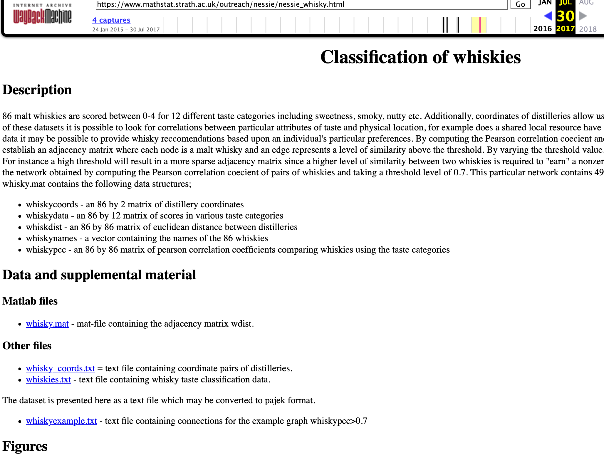
The Scottish Whiskey data set consist of tasting notes and evaluations from 86 distilleries around Scotland. This data set has been around a long time andwas a promotional site for a book, Whisky Classified: Choosing Single Malts by Flavour. Written by David Wishart of the University of Saint Andrews, the book had its most recent printing in February 2012.
I’ve been using this data set in one of my conference presentations (Planning my Summer Vacation), but to use this data set I need to add 2 new attributes/features to the data set. Each of the attributes are listed below and the last 2 are the attributes I added. These were added to include the converted LAT and LONG comparable with Google Maps and other similar mapping technology.
Attributes include:
- RowID
- Distillery
- Body
- Sweetness
- Smoky
- Medicinal
- Tobacco
- Honey
- Spicy
- Winey
- Nutty,
- Malty,
- Fruity,
- Floral,
- Postcode,
- Latitude,
- Longitude
- lat — newly added
- long — newly added
Here is the link to download and use this updated Scottish Whisky data set.
The original website is no longer available but if you have a look at the Internet Archive you will find the website.
Demographics vs Psychographics for Machine Learning
When preparing data for data science, data mining or machine learning projects you will create a data set that describes the various characteristics of the subject or case record. Each attribute will contain some descriptive information about the subject and is related to the target variable in some way.
In addition to these attributes, the data set will be enriched with various other internal/external data to complete the data set.
Some of the attributes in the data set can be grouped under the heading of Demographics. Demographic data contains attributes that explain or describe the person or event each case record is focused on. For example, if the subject of the case record is based on Customer data, this is the “Who” the demographic data (and features/attributes) will be about. Examples of demographic data include:
- Age range
- Marital status
- Number of children
- Household income
- Occupation
- Educational level
These features/attributes are typically readily available within your data sources and if they aren’t then these name be available from a purchased data set.
Additional feature engineering methods are used to generate new features/attributes that express meaning is different ways. This can be done by combining features in different ways, binning, dimensionality reduction, discretization, various data transformations, etc. The list can go on.
The aim of all of this is to enrich the data set to include more descriptive data about the subject. This enriched data set will then be used by the machine learning algorithms to find the hidden patterns in the data. The richer and descriptive the data set is the greater the likelihood of the algorithms in detecting the various relationships between the features and their values. These relationships will then be included in the created/generated model.
Another approach to consider when creating and enriching your data set is move beyond the descriptive features typically associated with Demographic data, to include Pyschographic data.
Psychographic data is a variation on demographic data where the feature are about describing the habits of the subject or customer. Demographics focus on the “who” while psycographics focus on the “why”. For example, a common problem with data sets is that they describe subjects/people who have things in common. In such scenarios we want to understand them at a deeper level. Psycographics allows us to do this. Examples of Psycographics include:
- Lifestyle activities
- Evening activities
- Purchasing interests – quality over economy, how environmentally concerned are you
- How happy are you with work, family, etc
- Social activities and changes in these
- What attitudes you have for certain topic areas
- What are your principles and beliefs
The above gives a far deeper insight into the subject/person and helps to differentiate each subject/person from each other, when there is a high similarity between all subjects in the data set. For example, demographic information might tell you something about a person’s age, but psychographic information will tell you that the person is just starting a family and is in the market for baby products.
I’ll close with this. Consider the various types of data gathering that companies like Google, Facebook, etc perform. They gather lots of different types of data about individuals. This allows them to build up a complete and extensive profile of all activities for individuals. They can use this to deliver more accurate marketing and advertising. For example, Google gathers data about what places to visit throughout a data, they gather all your search results, and lots of other activities. They can do a lot with this data. but now they own Fitbit. Think about what they can do with that data and particularly when combined with all the other data they have about you. What if they had access to your medical records too! Go Google this ! You will find articles about them now having access to your health records. Again combine all of the data from these different data sources. How valuable is that data?
Managing imbalanced Data Sets with SMOTE in Python
When working with data sets for machine learning, lots of these data sets and examples we see have approximately the same number of case records for each of the possible predicted values. In this kind of scenario we are trying to perform some kind of classification, where the machine learning model looks to build a model based on the input data set against a target variable. It is this target variable that contains the value to be predicted. In most cases this target variable (or feature) will contain binary values or equivalent in categorical form such as Yes and No, or A and B, etc or may contain a small number of other possible values (e.g. A, B, C, D).
For the classification algorithm to perform optimally and be able to predict the possible value for a new case record, it will need to see enough case records for each of the possible values. What this means, it would be good to have approximately the same number of records for each value (there are many ways to overcome this and these are outside the score of this post). But most data sets, and those that you will encounter in real life work scenarios, are never balanced, as in having a 50-50 split. What we typically encounter might be a 90-10, 98-2, etc type of split. These data sets are said to be imbalanced.

The image above gives examples of two approaches for creating a balanced data set. The first is under-sampling. This involves reducing the class that contains the majority of the case records and reducing it to match the number of case records in the minor class. The problems with this include, the resulting data set is too small to be meaningful, the case records removed could contain important records and scenarios that the model will need to know about.
The second example is creating a balanced data set by increasing the number of records in the minority class. There are a few approaches to creating this. The first approach is to create duplicate records, from the minor class, until such time as the number of case records are approximately the same for each class. This is the simplest approach. The second approach is to create synthetic records that are statistically equivalent of the original data set. A commonly technique used for this is called SMOTE, Synthetic Minority Oversampling Technique. SMOTE uses a nearest neighbors algorithm to generate new and synthetic data we can use for training our model. But one of the issues with SMOTE is that it will not create sample records outside the bounds of the original data set. As you can image this would be very difficult to do.
The following examples will illustrate how to perform Under-Sampling and Over-Sampling (duplication and using SMOTE) in Python using functions from Pandas, Imbalanced-Learn and Sci-Kit Learn libraries.
NOTE: The Imbalanced-Learn library (e.g. SMOTE)requires the data to be in numeric format, as it statistical calculations are performed on these. The python function get_dummies was used as a quick and simple to generate the numeric values. Although this is perhaps not the best method to use in a real project. With the other sampling functions can process data sets with a sting and numeric.
Data Set: Is the Portuaguese Banking data set and is available on the UCI Data Set Repository, and many other sites. Here are some basics with that data set.
import warnings

import pandas as pd
import numpy as np
import matplotlib.pyplot as plt
get_ipython().magic('matplotlib inline')

bank_file = ".../bank-additional-full.csv"

# import dataset
df = pd.read_csv(bank_file, sep=';',)

# get basic details of df (num records, num features)
df.shape
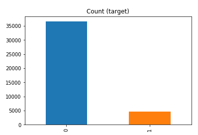
df['y'].value_counts() # dataset is imbalanced with majority of class label as "no".
no     36548
yes     4640
Name: y, dtype: int64
#print bar chart
df.y.value_counts().plot(kind='bar', title='Count (target)');
Example 1a – Down/Under sampling the majority class y=1 (using random sampling)
count_class_0, count_class_1 = df.y.value_counts()

# Divide by class
df_class_0 = df[df['y'] == 0] #majority class
df_class_1 = df[df['y'] == 1] #minority class

# Sample Majority class (y=0, to have same number of records as minority calls (y=1)
df_class_0_under = df_class_0.sample(count_class_1)
# join the dataframes containing y=1 and y=0
df_test_under = pd.concat([df_class_0_under, df_class_1])

print('Random under-sampling:')
print(df_test_under.y.value_counts())
print("Num records = ", df_test_under.shape[0])

df_test_under.y.value_counts().plot(kind='bar', title='Count (target)');

Example 1b – Down/Under sampling the majority class y=1 using imblearn
from imblearn.under_sampling import RandomUnderSampler

X = df_new.drop('y', axis=1)
Y = df_new['y']

rus = RandomUnderSampler(random_state=42, replacement=True)
X_rus, Y_rus = rus.fit_resample(X, Y)

df_rus = pd.concat([pd.DataFrame(X_rus), pd.DataFrame(Y_rus, columns=['y'])], axis=1)

print('imblearn over-sampling:')
print(df_rus.y.value_counts())
print("Num records = ", df_rus.shape[0])

df_rus.y.value_counts().plot(kind='bar', title='Count (target)');
[same results as Example 1a]
Example 1c – Down/Under sampling the majority class y=1 using Sci-Kit Learn
from sklearn.utils import resample

print("Original Data distribution")
print(df['y'].value_counts())

# Down Sample Majority class
down_sample = resample(df[df['y']==0],
replace = True, # sample with replacement
n_samples = df[df['y']==1].shape[0], # to match minority class
random_state=42) # reproducible results

# Combine majority class with upsampled minority class
train_downsample = pd.concat([df[df['y']==1], down_sample])

# Display new class counts
print('Sci-Kit Learn : resample : Down Sampled data set')
print(train_downsample['y'].value_counts())
print("Num records = ", train_downsample.shape[0])
train_downsample.y.value_counts().plot(kind='bar', title='Count (target)');
[same results as Example 1a]
Example 2 a – Over sampling the minority call y=0 (using random sampling)
df_class_1_over = df_class_1.sample(count_class_0, replace=True)
df_test_over = pd.concat([df_class_0, df_class_1_over], axis=0)

print('Random over-sampling:')
print(df_test_over.y.value_counts())

df_test_over.y.value_counts().plot(kind='bar', title='Count (target)');
Random over-sampling:
1    36548
0    36548
Name: y, dtype: int64

Example 2b – Over sampling the minority call y=0 using SMOTE
from imblearn.over_sampling import SMOTE

print(df_new.y.value_counts())
X = df_new.drop('y', axis=1)
Y = df_new['y']

sm = SMOTE(random_state=42)
X_res, Y_res = sm.fit_resample(X, Y)

df_smote_over = pd.concat([pd.DataFrame(X_res), pd.DataFrame(Y_res, columns=['y'])], axis=1)

print('SMOTE over-sampling:')
print(df_smote_over.y.value_counts())

df_smote_over.y.value_counts().plot(kind='bar', title='Count (target)');
[same results as Example 2a]
Example 2c – Over sampling the minority call y=0 using Sci-Kit Learn
from sklearn.utils import resample

print("Original Data distribution")
print(df['y'].value_counts())

# Upsample minority class
train_positive_upsample = resample(df[df['y']==1],
replace = True, # sample with replacement
n_samples = train_zero.shape[0], # to match majority class
random_state=42) # reproducible results

# Combine majority class with upsampled minority class
train_upsample = pd.concat([train_negative, train_positive_upsample])

# Display new class counts
print('Sci-Kit Learn : resample : Up Sampled data set')
print(train_upsample['y'].value_counts())
train_upsample.y.value_counts().plot(kind='bar', title='Count (target)');
[same results as Example 2a]
Oracle Text, Oracle R Enterprise and Oracle Data Mining – Part 4
This is the fourth blog post of a series on using Oracle Text, Oracle R Enterprise and Oracle Data Mining. Make sure to check out the previous blog posts as each one builds upon each other.
In this blog post, I will have an initial look at how you can use Oracle Text to perform document classification. In my next blog post, in the series, I will look at how you can use Oracle Data Mining with Oracle Text to perform classification.
The area of document classification using Oracle Text is a well trodden field and there are lots and lots of material out there to assist you. This blog post will look at the core steps you need to follow and how Oracle Text can help you with classifying your documents or text objects in a table.
When you use Oracle Text for documentation classification the simplest approach is to use ‘Rule-based Classification’. With this approach you will defined a set of rules, when applied to the document will determine classification that will be assigned to the document.
There is a little bit of setup and configuration needed to make this happen. This includes the following.
- Create a table that will store you document. See my previous blog posts in the series to see an example of one that is used to store the text from webpages.
- Create a rules table. This will contain the classification label and then a set of rules that will be used by Oracle Text to determine that classification to assign to the document. These are in the format similar to what you might see in the WHERE clause of a SELECT statement. You will need follow the rules and syntax of CTXRULES to make sure your rules fire correctly.
- Create a CTXRULE index on the rules table you created in the previous step.
- Create a table that will be a link table between the table that contains your documents and the table that contains your categories.
When you have these steps completed you can now start classifying your documents. The following example illustrates using these steps using the text documents I setup in my previous blog posts.
Here is the structure of my documents table. I had also created an Oracle Text CTXSYS.CONTEXT index on the DOC_TEXT attribute.
create table MY_DOCUMENTS (
 doc_pk			NUMBER(10) PRIMARY KEY,
 doc_title		VARCHAR2(100),
 doc_extracted 	DATE,
 data_source 	VARCHAR2(200),
 doc_text 		CLOB );
The next step is to create a table that contains our categories and rules. The structure of this table is very simple, and the following is an example.
create table DOCUMENT_CATEGORIES (
 doc_cat_pk  	NUMBER(10) PRIMARY KEY,
 doc_category 	VARCHAR2(40),
 doc_cat_query  VARCHAR2(2000) );

create sequence doc_cat_seq;
Now we can create the table that will store the identified document categories/classifications for each of out documents. This is a link table that contains the primary keys from the MY_DOCUMENTS and the MY_DOCUMENT_CATEGORIES tables.
create table MY_DOC_CAT (
 doc_pk 	NUMBER(10),
 doc_cat_pk NUMBER(10) );
Queries for CTXRULE are similar to those of CONTAINS queries. Basic phrasing within quotes is supported, as are the following CONTAINS operators: ABOUT, AND, NEAR, NOT, OR, STEM, WITHIN, and THESAURUS. The following statements contain my rules.
insert into document_categories values
  (doc_cat_seq.nextval, 'OAA','Oracle Advanced Analytics');

insert into document_categories values
  (doc_cat_seq.nextval, 'Oracle Data Mining','ODM or Oracle Data Mining');

insert into document_categories values
  (doc_cat_seq.nextval, 'Oracle Data Miner','ODMr or Oracle Data Miner or SQL Developer');

insert into document_categories values
  (doc_cat_seq.nextval, 'R Technologies','Oracle R Enterprise or ROacle or ORAACH or R');
We are now ready to create the Oracle Text CTXRULE index.
create index doc_cat_idx on document_categories(doc_cat_query) indextype is ctxsys.ctxrule;
Our next step is to apply the rules and to generate the categories/classifications. We have two scenarios to deal with here. The first is how do we do this for our existing records and the second to how can you do this ongoing as new documents get loaded into the MY_DOCUMENTS table.
For the first scenario, where the documents already exist in our table, we can can use a procedure, just like the following.
DECLARE
   v_document    MY_DOCUMENTS.DOC_TEXT%TYPE;
   v_doc         MY_DOCUMENTS.DOC_PK%TYPE;
BEGIN
   for doc in (select doc_pk, doc_text from my_documents) loop
      v_document := doc.doc_text;
      v_doc  := doc.doc_pk;
      for c in (select doc_cat_pk from document_categories
              where matches(doc_cat_query, v_document) > 0 )
         loop
            insert into my_doc_cat values (doc.doc_pk, c.doc_cat_pk);
      end loop;
   end loop;
END;
/
Let us have a look at the categories/classifications that were generated.
select a.doc_title, c.doc_cat_pk, b.doc_category
from my_documents a,
     document_categories b,
     my_doc_cat c
where a.doc_pk = c.doc_pk
and c.doc_cat_pk = b.doc_cat_pk
order by a.doc_pk, c.doc_cat_pk;

We can see the the categorisation/classification actually gives us the results we would have expected of these documents/web pages.
Now we can look at how to generate these these categories/classifications on an on going basis. For this we will need a database trigger on the MY_DOCUMENTS table. Something like the following should do the trick.
CREATE or REPLACE TRIGGER t_cat_doc
  before insert on MY_DOCUMENTS
  for each row
BEGIN
  for c in (select doc_cat_pk from document_categories
            where  matches(doc_cat_query, :new.doc_text)>0)
  loop
        insert into my_doc_cat values (:new.doc_pk, c.doc_cat_pk);
  end loop;
END;
At this point we have now worked through how to build and use Oracle Text to perform Rule based document categorisation/classification.
In addition to this type of classification, Oracle Text also has uses some machine learning algorithms to classify documents. These include using Decision Trees, Support Vector Machines and Clustering. It is important to note that these are not the machine learning algorithms that come as part of Oracle Data Mining. Look out of my other blog posts that cover these topics.
Cluster Distance using SQL with Oracle Data Mining – Part 4
This is the fourth and last blog post in a series that looks at how you can examine the details of predicted clusters using Oracle Data Mining. In the previous blog posts I looked at how to use CLUSER_ID, CLUSTER_PROBABILITY and CLUSTER_SET.
In this blog post we will look at CLUSTER_DISTANCE. We can use the function to determine how close a record is to the centroid of the cluster. Perhaps we can use this to determine what customers etc we might want to focus on most. The customers who are closest to the centroid are one we want to focus on first. So we can use it as a way to prioritise our workflows, particularly when it is used in combination with the value for CLUSTER_PROBABILITY.
Here is an example of using CLUSTER_DISTANCE to list all the records that belong to Cluster 14 and the results are ordered based on closeness to the centroid of this cluster.
SELECT customer_id,
       cluster_probability(clus_km_1_37 USING *) as cluster_Prob,
       cluster_distance(clus_km_1_37 USING *) as cluster_Distance
FROM   insur_cust_ltv_sample
WHERE   cluster_id(clus_km_1_37 USING *) = 14
order by cluster_Distance asc;
Here is a subset of the results from this query.

When you examine the results you may notice that the records that is listed first and closest record to the centre of cluster 14 has a very low probability. You need to remember that we are working in a N-dimensional space here. Although this first record is closest to the centre of cluster 14 it has a really low probability and if we examine this record in more detail we will find that it is at an overlapping point between a number of clusters.
This is why we need to use the CLUSTER_DISTANCE and CLUSTER_PROBABILITY functions together in our workflows and applications to determine how we need to process records like these.
Cluster Sets using SQL with Oracle Data Mining – Part 3
This is the third blog post on my series on examining the Clusters that were predicted by an Oracle Data Mining model. Check out the previous blog posts.
- Part 1 – Examining predicted Clusters and Cluster details using SQL
- Part 2 – Cluster Details with Oracle Data Mining
In the previous posts we were able to list the predicted cluster for each record in our data set. This is the cluster that the records belonged to the most. I also mentioned that a record could belong to many clusters.
So how can you list all the clusters that the a record belongs to?
You can use the CLUSTER_SET SQL function. This will list the Cluster Id and a probability measure for each cluster. This function returns a array consisting of the set of all clusters that the record belongs to.
The following example illustrates how to use the CLUSTER_SET function for a particular cluster model.
SELECT t.customer_id, s.cluster_id, s.probability
FROM   (select customer_id, cluster_set(clus_km_1_37 USING *) as Cluster_Set
        from   insur_cust_ltv_sample
        WHERE  customer_id in ('CU13386', 'CU100')) T,
      TABLE(T.cluster_set) S
order by t.customer_id, s.probability desc;
The output from this query will be an ordered data set based on the customer id and then the clusters listed in descending order of probability. The cluster with the highest probability is what would be returned by the CLUSTER_ID function. The output from the above query is shown below.

If you would like to see the details of each of the clusters and to examine the differences between these clusters then you will need to use the CLUSTER_DETAILS function (see previous blog post).
You can specify topN and cutoff to limit the number of clusters returned by the function. By default, both topN and cutoff are null and all clusters are returned.
– topN is the N most probable clusters. If multiple clusters share the Nth probability, then the function chooses one of them.
– cutoff is a probability threshold. Only clusters with probability greater than or equal to cutoff are returned. To filter by cutoff only, specify NULL for topN.
You may want to use these individually or combined together if you have a large number of customers. To return up to the N most probable clusters that are greater than or equal to cutoff, specify both topN and cutoff.
The following example illustrates using the topN value to return the top 4 clusters.
SELECT t.customer_id, s.cluster_id, s.probability
FROM   (select customer_id, cluster_set(clus_km_1_37, 4, null USING *) as Cluster_Set
        from   insur_cust_ltv_sample
        WHERE  customer_id in ('CU13386', 'CU100')) T,
      TABLE(T.cluster_set) S
order by t.customer_id, s.probability desc;
and the output from this query shows only 4 clusters displayed for each record.

Alternatively you can select the clusters based on a cut off value for the probability. In the following example this is set to 0.05.
SELECT t.customer_id, s.cluster_id, s.probability
FROM   (select customer_id, cluster_set(clus_km_1_37, NULL, 0.05 USING *) as Cluster_Set
        from   insur_cust_ltv_sample
        WHERE  customer_id in ('CU13386', 'CU100')) T,
      TABLE(T.cluster_set) S
order by t.customer_id, s.probability desc;
and the output this time looks a bit different.

Finally, yes you can combine these two parameters to work together.
SELECT t.customer_id, s.cluster_id, s.probability
FROM (select customer_id, cluster_set(clus_km_1_37, 2, 0.05 USING *) as Cluster_Set
from insur_cust_ltv_sample
WHERE customer_id in (‘CU13386’, ‘CU100’)) T,
TABLE(T.cluster_set) S
order by t.customer_id, s.probability desc;
PMML in Oracle Data Mining
PMML (Predictive Model Markup Langauge) is an XML formatted output that defines the core elements and settings for your Predictive Models. This XML formatted output can be used to migrate your models from one data mining or predictive modelling tool to another data mining or predictive modelling tool, such as Oracle.
Using PMML to migrate your models from one tool to another allows for you to use the most appropriate tools for developing your models and then allows them to be imported into another tool that will be used for deploying your predictive models in batch or real-time mode. In particular the ability to use your Predictive Model within your everyday applications enables you to work in the area of Automatic or Prescriptive Analytics. Oracle Data Mining and the Oracle Database are ideal or even the best possible tools to allow for Automatic and Prescriptive Analytics for your transa
PMML is an XML based standard specified by the Data Mining Group
Oracle Data Mining supports the importing of PMML models that are compliant with version 3.1 of the standard and for Regression Models only. The regression models can be for linear regression or binary logistic regression.
The Data Mining Group Archive webpage have a number of sample PMML files for you to download and then to load into your Oracle database.
To Load the PMML file into your Oracle Database you can use the DBMS_DATA_MINING.IMPORT_MODEL function. I’ve given examples of how you can use this function to import an Oracle Data Mining model that was exported using the EXPORT_MODEL function.
The syntax of the IMPORT_MODEL function when importing a PMML file is the following
DBMS_DATA_MINING.IMPORT_MODEL (
      model_name        IN  VARCHAR2,
      pmmldoc           IN  XMLTYPE
      strict_check      IN  BOOLEAN DEFAULT FALSE);
The following example shows how you can load the version 3.1 Logistic Regression PMML file from the Data Mining Group archive webpage
![]()
BEGIN
   dbms_data_mining.IMPORT_MODEL (‘PMML_MODEL',
        XMLType (bfilename (‘IMPORT_DIR', 'sas_3.1_iris_logistic_reg.xml'),
          nls_charset_id ('AL32UTF8')
        ));
END;
This example uses the default value for STRICT_CHECK as FALASE. In this case if there are any errors in the PMML structure then these will be ignored and the imported model may contain “features” that may make it perform in a slightly odd manner.

You must be logged in to post a comment.