
Oracle Database
Oracle Semantic Search using Vectors on Iceberg Tables
In my previous blog posts I’ve explored how to use Iceberg Tables and how to integrate these in with your Data Lake. Additionally, I showed how to setup your Oracle Data Lake (Database) to access the data stored in Iceberg Tables stored in OCI Object Storage. To access this Iceberg Table data from the Oracle Database we created an External Table. This allows us to query the Iceberg Table data as if it was internal to the database. With all new releases there is continuous improvement in the features and to make them easier to use. One such new feature (as of 23.26.1) is the ability to read vector data types from an External Table. This new feature is called or referred to as ‘Vectors on Ice’.
With Oracle Database External Tables now supporting vector embedding stored in Iceberg Tables, means you can generate vector embeddings with your preferred embedding model (external to Oracle using your faviourite tool/library), store them in Iceberg Tables in cloud object storage (OCI Object Storage, AWS S3, etc.), and run semantic search from Oracle AI Database, accessing vector data stored within the database and externally with the minimum of data movement and with similar SQL queries.
Summary: Vectors on Ice lets you ask semantic questions of your data lake using the same SQL and vector search tooling you already use in Oracle Database, without copying or moving the data.
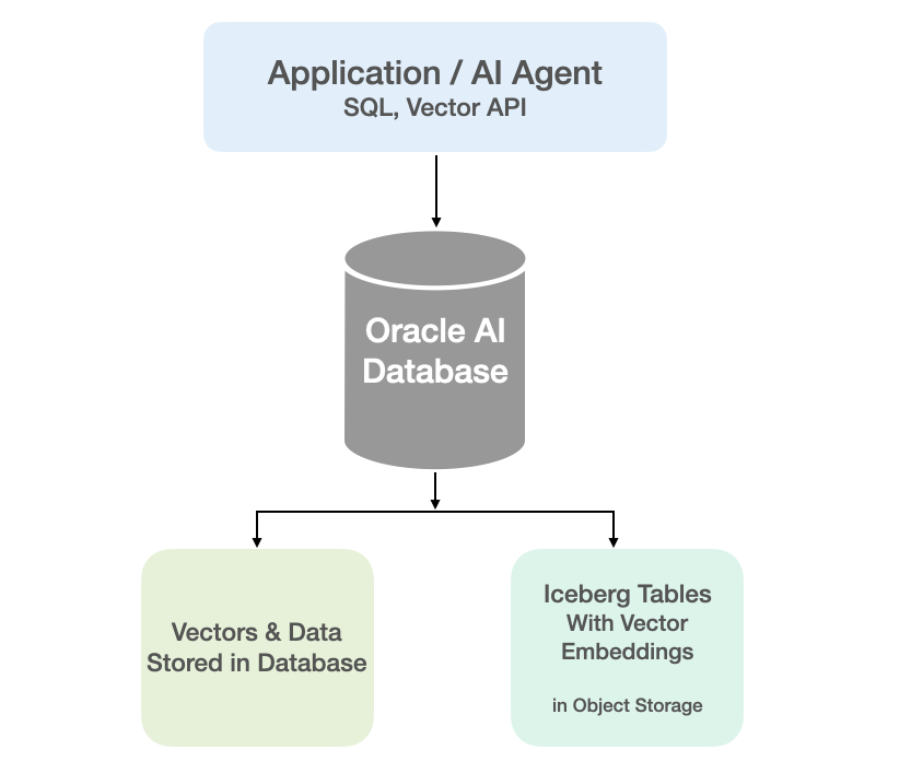
Oracle vector indexes can be created to speed up semantic search over the vectors in the Iceberg Tables. You don’t need to copy Iceberg data into an Oracle Database to use them or to update the Vector Index. The vector indexes are stored standalone in the database and (depending on the type of Vector Index used) can automatic sync as data is added to the files on Object Storage. The syncing of the Vector Index is not immediately updated but is updated based on a background process, so you can look on this index being eventually consistent. In might happen fairly quickly or during large write periods in might take seconds to a few minutes to get fully up-to-date.
Let’s have a look at an example of this. The following example builds upon my example in my previous posts which walked through the setup sets needed for gaining access to Object Storage, etc
CREATE TABLE IF NOT EXISTS external_vector_file ( id VARCHAR(10) PRIMARY KEY, text_desc VARCHAR2(1000), vec_embedding VECTOR(1024, float32) ) ORGANIZATION EXTERNAL ( TYPE ORACLE_BIGDATA DEFAULT DIRECTORY DATA_PUMP_DIR ACCESS PARAMETERS ( com.oracle.bigdata.credential.name=OCI_CRED com.oracle.bigdata.fileformat=parquet com.oracle.bigdata.access_protocol=iceberg ) LOCATION ('<path-to-iceberg-table>/metadata/v1.metadata.json') ) REJECT LIMIT UNLIMITED;
and to create a Vector Index on this external file
CREATE VECTOR INDEX external_vector_file_idx_ivf ON external_vector_file (vec_embedding)ORGANIZATION NEIGHBOR PARTITIONS;
We can now run our SQL queries on this external vector data. This query assumes we have the same vector embedding model loaded into the database.
SELECT id, text_desc, vector_distance(vec_embedding, vector_embedding(my_onnx_model using :INPUT_TERM as data) DISTFROM external_vector_fileORDER BY DISTFETCH FIRST 10 ROWS ONLY;
Why is this important? This allows organisations that already store vectors or embeddings in Iceberg Tables, as part of an existing ML pipeline, and who want to query them, performing semantic search, alongside the data in their Oracle Database, can now do so with the minimum of setup. This brings the benefits of Semantic Search to a wider audience within the organisation.
Oracle 23c DBMS_SEARCH – Ubiquitous Search
One of the new PL/SQL packages with Oracle 23c is DBMS_SEARCH. This can be used for indexing (and searching) multiple schema objects in a single index.
Check out the documentation for DBMS_SEARCH.
This type of index is a little different to your traditional index. With DBMS_SEARCH we can create an index across multiple schema objects using just a single index. This gives us greater indexing capabilities for scenarios where we need to search data across multiple objects. You can create a ubiquitous search index on multiple columns of a table or multiple columns from different tables in a given schema. All done using one index, rather than having to use multiples. Because of this wider search capability, you will see this (DBMS_SEARCH) being referred to as a Ubiquitous Search Index. A ubiquitous search index is a JSON search index and can be used for full-text and range-based searches.
To create the index, you will first define the name of the index, and then add the different schema objects (tables, views) to it. The main commands for creating the index are:
- DBMS_SEARCH.CREATE_INDEX
- DBMS_SEARCH.ADD_SOURCE
Note: Each table used in the ADD_SOURCE must have a primary key.
The following is an example of using this type of index using the HR schema/data set.
exec dbms_search.create_index('HR_INDEX');This just creates the index header.
Important: For each index created using this method it will create a table with the Index name in your schemas. It will also create fourteen DR$ tables in your schema. SQL Developer filtering will help to hide these and minimise the clutter.
select table_name from user_tables;
...
HR_INDEX
DR$HR_INDEX$I
DR$HR_INDEX$K
DR$HR_INDEX$N
DR$HR_INDEX$U
DR$HR_INDEX$Q
DR$HR_INDEX$C
DR$HR_INDEX$B
DR$HR_INDEX$SN
DR$HR_INDEX$SV
DR$HR_INDEX$ST
DR$HR_INDEX$G
DR$HR_INDEX$DG
DR$HR_INDEX$KG
To add the contents and search space to the index we need to use ADD_SOURCE. In the following, I’m adding two tables to the index.
exec DBMS_SEARCH.ADD_SOURCE('HR_INDEX', 'EMPLOYEES');NOTE: At the time of writing this post some of the client tools and libraries do not support the JSON datatype fully. If they did, you could just query the index metadata, but until such time all tools and libraries fully support the data type, you will need to use the JSON_SERIALIZE function to translate the metadata. If you query the metadata and get no data returned, then try using this function to get the data.
Running a simple select from the index might give you an error due to the JSON type not being fully implemented in the client software. (This will change with time)
select * from HR_INDEX;But if we do a count from the index, we could get the number of objects it contains.
select count(*) from HR_INDEX;
   COUNT(*)
___________
        107
We can view what data is indexed by viewing the virtual document.
select json_serialize(DBMS_SEARCH.GET_DOCUMENT('HR_INDEX',METADATA))
from HR_INDEX;

JSON_SERIALIZE(DBMS_SEARCH.GET_DOCUMENT('HR_INDEX',METADATA))
___________________________________________________________________________________________________________________________________________________________________________________________________________________________________________________________________________
{"HR":{"EMPLOYEES":{"PHONE_NUMBER":"515.123.4567","JOB_ID":"AD_PRES","SALARY":24000,"COMMISSION_PCT":null,"FIRST_NAME":"Steven","EMPLOYEE_ID":100,"EMAIL":"SKING","LAST_NAME":"King","MANAGER_ID":null,"DEPARTMENT_ID":90,"HIRE_DATE":"2003-06-17T00:00:00"}}}
{"HR":{"EMPLOYEES":{"PHONE_NUMBER":"515.123.4568","JOB_ID":"AD_VP","SALARY":17000,"COMMISSION_PCT":null,"FIRST_NAME":"Neena","EMPLOYEE_ID":101,"EMAIL":"NKOCHHAR","LAST_NAME":"Kochhar","MANAGER_ID":100,"DEPARTMENT_ID":90,"HIRE_DATE":"2005-09-21T00:00:00"}}}
{"HR":{"EMPLOYEES":{"PHONE_NUMBER":"515.123.4569","JOB_ID":"AD_VP","SALARY":17000,"COMMISSION_PCT":null,"FIRST_NAME":"Lex","EMPLOYEE_ID":102,"EMAIL":"LDEHAAN","LAST_NAME":"De Haan","MANAGER_ID":100,"DEPARTMENT_ID":90,"HIRE_DATE":"2001-01-13T00:00:00"}}}
{"HR":{"EMPLOYEES":{"PHONE_NUMBER":"590.423.4567","JOB_ID":"IT_PROG","SALARY":9000,"COMMISSION_PCT":null,"FIRST_NAME":"Alexander","EMPLOYEE_ID":103,"EMAIL":"AHUNOLD","LAST_NAME":"Hunold","MANAGER_ID":102,"DEPARTMENT_ID":60,"HIRE_DATE":"2006-01-03T00:00:00"}}}
{"HR":{"EMPLOYEES":{"PHONE_NUMBER":"590.423.4568","JOB_ID":"IT_PROG","SALARY":6000,"COMMISSION_PCT":null,"FIRST_NAME":"Bruce","EMPLOYEE_ID":104,"EMAIL":"BERNST","LAST_NAME":"Ernst","MANAGER_ID":103,"DEPARTMENT_ID":60,"HIRE_DATE":"2007-05-21T00:00:00"}}}
We can search the metadata for certain data using the CONTAINS or JSON_TEXTCONTAINS functions.
select json_serialize(metadata)
from DEMO_IDX
where contains(data, 'winston')>0;
select json_serialize(metadata)
from DEMO_IDX
where json_textcontains(data, '$.HR.EMPLOYEES.FIRST_NAME', 'Winston');When the index is no longer required it can be dropped by running the following. Don’t run a DROP INDEX command as that removes some objects and leaves others behind! (leaves a bit of mess) and you won’t be able to recreate the index, unless you give it a different name.
exec dbms_search.drop_index('SH_INDEX');Oracle Database In-Memory – simple example
In a previous post, I showed how to enable and increase the memory allocation for use by Oracle In-Memory. That example was based on using the Pre-built VM supplied by Oracle.
To use In-Memory on your objects, you have a few options.
Enabling the In-Memory attribute on the EXAMPLE tablespace by specifying the INMEMORY attribute
SQL> ALTER TABLESPACE example INMEMORY;Enabling the In-Memory attribute on the sales table but excluding the “prod_id” column
SQL> ALTER TABLE sales INMEMORY NO INMEMORY(prod_id);Disabling the In-Memory attribute on one partition of the sales table by specifying the NO INMEMORY clause
SQL> ALTER TABLE sales MODIFY PARTITION SALES_Q1_1998 NO INMEMORY;Enabling the In-Memory attribute on the customers table with a priority level of critical
SQL> ALTER TABLE customers INMEMORY PRIORITY CRITICAL;You can also specify the priority level, which helps to prioritise the order the objects are loaded into memory.

A simple example to illustrate the effect of using In-Memory versus not.
Create a table with, say, 11K records. It doesn’t really matter what columns and data are.
Now select all the records and display the explain plan
select count(*) from test_inmemory;
Now, move the table to In-Memory and rerun your query.
alter table test_inmemory inmemory PRIORITY critical;
select count(*) from test_inmemory;  -- again
There you go!
We can check to see what object are In-Memory by
SELECT table_name, inmemory, inmemory_priority, inmemory_distribute,
       inmemory_compression, inmemory_duplicate
FROM user_tables
WHERE inmemory = 'ENABLED’
ORDER BY table_name;
To remove the object from In-Memory
SQL > alter table test_inmemory no inmemory; -- remove the table from in-memory
This is just a simple test and lots of other things can be done to improve performance
But, you do need to be careful about using In-Memory. It does have some limitations and scenarios where it doesn’t work so well. So care is needed
Changing In-Memory size in Oracle Database
The pre-built virtual machine provided by Oracle for trying out and playing with Oracle Database comes configured to use the In-Memory option. But memory size is a little limited if you are trying to load anything slightly bigger than a tiny table into memory, for example if the table has more than a few hundred rows.
The amount of memory allocated to In-Memory can be increased to allow for more data to be loaded. There is a requirement that the VM and Database has enough memory allocated to allow this. If you don’t and increase the In-Memory size too large, you will have some problems restarting the database and VM. So proceed carefully.
For the pre-built VM, I typically allocate 4G or 8G of RAM to the VM. This in turn will give more memory to the database when it starts.
To setup In-Memory on the VM run the following:
– Open a terminal window and run this command:
sqlplus sys/oracle as sysdbaThen run these two commands
alter session set container = cdb$root;
alter system set inmemory_size = 200M scope=spfile;
Now, bounce the VM, i.e. restart the VM
In-memory will now be enabled on your Database, and you can now create/move tables in and out of in-memory.
Working with External Data on Oracle DB Docker
With multi-modal databases (such as Oracle and many more) you will typically work with data in different formats and for different purposes. One such data format is with data located external to the database. The data will exist in files on the operating systems on the DB server or on some connected storage device.
The following demonstrates how to move data to an Oracle Database Docker image and access this data using External Tables. (This based on an example from Oracle-base.com with a few additional commands).
For this example, I’ll be using an Oracle 21c Docker image setup previously. Similarly the same steps can be followed for the 18c XE Docker image, by changing the Contain Id from 21cFull to 18XE.
Step 1 – Connect to OS in the Docker Container & Create Directory
The first step involves connecting the the OS of the container. As the container is setup for default user ‘oracle’, that is who we will connect as, and it is this Linux user who owns all the Oracle installation and associated files and directories
docker exec -it 21cFull /bin/bash
When connected we are in the Home directory for the Oracle user.
The Home directory contains lots of directories which contain all the files necessary for running the Oracle Database.
Next we need to create a directory which will story the files.
mkdir ext_data
As we are logged in as the oracle Linux user, we don’t have to make any permissions changes, as Oracle Database requires read and write access to this directory.
Step 3 – Upload files to Directory on Docker container
Open another terminal window on your computer (desktop/laptop). You should have two such terminal windows open. One you opened for Step 1 above, and this one. This will allow you to easily switch between files on your computer and the files in the Docker container.
Download the two Countries files, to your computer, which are listed on Oracle-base.com. Countries1.txt and Countries2.txt.
Now you need to upload those files to the Docker container.
docker cp Countries1.txt 21cFull:/opt/oracle/ext_data/Countries1.txt
docker cp Countries2.txt 21cFull:/opt/oracle/ext_data/Countries2.txt
Step 4 – Connect to System (DBA) schema, Create User, Create Directory, Grant access to Directory
If you a new to the Database container, you don’t have any general users/schemas created. You should create one, as you shouldn’t use the System (or DBA) user for any development work. To create a new database user connect to System.
sqlplus system/SysPassword1@//localhost/XEPDB1
To use sqlplus command line tool you will need to install Oracle Instant Client and then SQLPlus (which is a separate download from the same directory for your OS)
To create a new user/schema in the database you can run the following (change the username and password to something more sensible).
create user brendan identified by BtPassword1
default tablespace users
temporary tablespace temp;
grant connect, resource to brendan;
alter user brendan
quota unlimited on users;
Now create the Directory object in the database, which points to the directory on the Docker OS we created in the Step 1 above. Grant ‘brendan’ user/schema read and write access to this Directory
CREATE OR REPLACE DIRECTORY ext_tab_data AS '/opt/oracle/ext_data';
grant read, write on directory ext_tab_data to brendan;
Now, connect to the brendan user/schema.
Step 5 – Create external table and test
To connect to brendan user/schema, you can run the following if you are still using SQLPlus
SQL> connect brendan/BtPassword1@//localhost/XEPDB1
or if you exited it, just run this from the command line
sqlplus system/SysPassword1@//localhost/XEPDB1
Create the External Table (same code from oracle-base.com)
CREATE TABLE countries_ext (
  country_code      VARCHAR2(5),
  country_name      VARCHAR2(50),
  country_language  VARCHAR2(50)
)
ORGANIZATION EXTERNAL (
  TYPE ORACLE_LOADER
  DEFAULT DIRECTORY ext_tab_data
  ACCESS PARAMETERS (
    RECORDS DELIMITED BY NEWLINE
    FIELDS TERMINATED BY ','
    MISSING FIELD VALUES ARE NULL
    (
      country_code      CHAR(5),
      country_name      CHAR(50),
      country_language  CHAR(50)
    )
  )
  LOCATION ('Countries1.txt','Countries2.txt')
)
PARALLEL 5
REJECT LIMIT UNLIMITED;
It should create for you. If not and you get an error then if will be down to a typo on directory name or the files are not in the directory or something like that.
We can now query the External Table as if it is a Table in the database.
SQL> set linesize 120
SQL> select * from countries_ext order by country_name;
COUNT COUNTRY_NAME                         COUNTRY_LANGUAGE
----- ------------------------------------ ------------------------------
ENG   England                              English
FRA   France                               French
GER   Germany                              German
IRE   Ireland                              English
SCO   Scotland                             English
USA   Unites States of America             English
WAL   Wales                                Welsh

7 rows selected.
All done!
GoLang: Inserting records into Oracle Database using goracle
In this blog post I’ll give some examples of how to process data for inserting into a table in an Oracle Database. I’ve had some previous blog posts on how to setup and connecting to an Oracle Database, and another on retrieving data from an Oracle Database and the importance of setting the Array Fetch Size.
When manipulating data the statements can be grouped (generally) into creating new data and updating existing data.
When working with this kind of processing we need to avoid the creation of the statements as a concatenation of strings. This opens the possibility of SQL injection, plus we are not allowing the optimizer in the database to do it’s thing. Prepared statements allows for the reuse of execution plans and this in turn can speed up our data processing and applications.
In a previous blog post I gave a simple example of a prepared statement for querying data and then using it to pass in different values as a parameter to this statement.
dbQuery, err := db.Prepare("select cust_first_name, cust_last_name, cust_city from sh.customers where cust_gender = :1")
if err != nil {
    fmt.Println(err)
    return
}
defer dbQuery.Close()

rows, err := dbQuery.Query('M')
if err != nil {
    fmt.Println(".....Error processing query")
    fmt.Println(err)
    return
}
defer rows.Close()

var CustFname, CustSname,CustCity string
for rows.Next() {
    rows.Scan(&CustFname, &CustSname, &CustCity)
    fmt.Println(CustFname, CustSname, CustCity)
}
For prepared statements for inserting data we can follow a similar structure. In the following example a table call LAST_CONTACT is used. This table has columns:
- CUST_ID
- CON_METHOD
- CON_MESSAGE
_, err := db.Exec("insert into LAST_CONTACT(cust_id, con_method, con_message) VALUES(:1, :2, :3)", 1, "Phone", "First contact with customer")
if err != nil {
    fmt.Println(".....Error Inserting data")
    fmt.Println(err)
    return
}
an alternative is the following and allows us to get some additional information about what was done and the result from it. In this example we can get the number records processed.
stmt, err := db.Prepare("insert into LAST_CONTACT(cust_id, con_method, con_message) VALUES(:1, :2, :3)")
if err != nil {
    fmt.Println(err)
    return
}

res, err := dbQuery.Query(1, "Phone", "First contact with customer")
if err != nil {
    fmt.Println(".....Error Inserting data")
    fmt.Println(err)
    return
}

rowCnt := res.RowsAffected()
fmt.Println(rowCnt, " rows inserted.")
A similar approach can be taken for updating and deleting records
Managing Transactions
With transaction, a number of statements needs to be processed as a unit. For example, in double entry book keeping we have two inserts. One Credit insert and one debit insert. To do this we can define the start of a transaction using db.Begin() and the end of the transaction with a Commit(). Here is an example were we insert two contact details.
// start the transaction
transx, err := db.Begin()
if err != nil {
    fmt.Println(err)
    return
}

// Insert first record
_, err := db.Exec("insert into LAST_CONTACT(cust_id, con_method, con_message) VALUES(:1, :2, :3)", 1, "Email", "First Email with customer")
if err != nil {
    fmt.Println(".....Error Inserting data - first statement")
    fmt.Println(err)
    return
}
// Insert second record
_, err := db.Exec("insert into LAST_CONTACT(cust_id, con_method, con_message) VALUES(:1, :2, :3)", 1, "In-Person", "First In-Person with customer")
if err != nil {
    fmt.Println(".....Error Inserting data - second statement")
    fmt.Println(err)
    return
}

// complete the transaction
err = transx.Commit()
if err != nil {
    fmt.Println(".....Error Committing Transaction")
    fmt.Println(err)
    return
}
GoLang: Querying records from Oracle Database using goracle
Continuing my series of blog posts on using Go Lang with Oracle, in this blog I’ll look at how to setup a query, run the query and parse the query results. I’ll give some examples that include setting up the query as a prepared statement and how to run a query and retrieve the first record returned. Another version of this last example is a query that returns one row.
Check out my previous post on how to create a connection to an Oracle Database.
Let’s start with a simple example. This is the same example from the blog I’ve linked to above, with the Database connection code omitted.
    dbQuery := "select table_name from user_tables where table_name not like 'DM$%' and table_name not like 'ODMR$%'"
    rows, err := db.Query(dbQuery)
    if err != nil {
        fmt.Println(".....Error processing query")
        fmt.Println(err)
        return
    }
    defer rows.Close()

    fmt.Println("... Parsing query results")
    var tableName string
    for rows.Next() {
        rows.Scan(&tableName)
        fmt.Println(tableName)
    }
Processing a query and it’s results involves a number of steps and these are:
- Using Query() function to send the query to the database. You could check for errors when processing each row
- Iterate over the rows using Next()
- Read the columns for each row into variables using Scan(). These need to be defined because Go is strongly typed.
- Close the query results using Close(). You might want to defer the use of this function but depends if the query will be reused. The result set will auto close the query after it reaches the last records (in the loop). The Close() is there just in case there is an error and cleanup is needed.
You should never use * as a wildcard in your queries. Always explicitly list the attributes you want returned and only list the attributes you want/need. Never list all attributes unless you are going to use all of them. There can be major query performance benefits with doing this.
Now let us have a look at using prepared statement. With these we can parameterize the query giving us greater flexibility and reuse of the statements. Additionally, these give use better query execution and performance when run the the database as the execution plans can be reused.
    dbQuery, err := db.Prepare("select cust_first_name, cust_last_name, cust_city from sh.customers where cust_gender = :1")
    if err != nil {
        fmt.Println(err)
        return
    }
    defer dbQuery.Close()

    rows, err := dbQuery.Query('M')
    if err != nil {
        fmt.Println(".....Error processing query")
        fmt.Println(err)
        return
    }
    defer rows.Close()

    var CustFname, CustSname,CustCity string
    for rows.Next() {
        rows.Scan(&CustFname, &CustSname, &CustCity)
        fmt.Println(CustFname, CustSname, CustCity)
    }
Sometimes you may have queries that return only one row or you only want the first row returned by the query. In cases like this you can reduce the code to something like the following.
var CustFname, CustSname,CustCity string
err := db.Prepare("select cust_first_name, cust_last_name, cust_city from sh.customers where cust_gender = ?").Scan(&CustFname, &CustSname, &CustCity)
if err != nil {
    fmt.Println(err)
    return
}
fmt.Println(CustFname, CustSname, CustCity)
or an alternative to using Quer(), use QueryRow()
dbQuery, err := db.Prepare("select cust_first_name, cust_last_name, cust_city from sh.customers where cust_gender = ?")
if err != nil {
    fmt.Println(err)
    return
}
defer dbQuery.Close()

var CustFname, CustSname,CustCity string
err := dbQuery.QueryRow('M').Scan(&CustFname, &CustSname, &CustCity)
if err != nil {
    fmt.Println(".....Error processing query")
    fmt.Println(err)
    return
}
fmt.Println(CustFname, CustSname, CustCity)
Importance of setting Fetched Rows size for Database Query using Golang
When issuing queries to the database one of the challenges every developer faces is how to get the results quickly. If your queries are only returning a small number of records, eg. < 5, then you don’t really have to worry about execution time. That is unless your query is performing some complex processing, joining lots of tables, etc.
Most of the time developers are working with one or a small number of records, using a simple query. Everything runs quickly.
But what if your query is returning several tens or thousands of records. Assuming we have a simple query and no query optimization is needed, the challenge facing the developer is how can you get all of those records quickly into your environment and process them. Typically the database gets blamed for the query result set being returned slowly. But what if this wasn’t the case? In most cases developers take the default parameter settings of the functions and libraries. For database connection libraries and their functions, you can change some of the parameters and affect how your code, your query, gets executed on the Database server and can affect how quickly the data is shipped from the database to your code.
One very important parameter to consider is the query array size. This is the number of records the database will send to your code in each batch. The database will keep sending batches until you tell it to stop. It makes sense to have the size of this batch set to a small value, as most queries return one or a small number of records. But when we get onto returning a larger number of records it can affect the response time significantly.
I tested the effect of changing the size of the returning buffer/array using Golang and querying data in an Oracle Database, hosted on Oracle Cloud, and using goracle library to connect to the database.
[ I did a similar test using Python. The results can be found here. You will notices that Golang is significantly quicker than Python, as you would expect. ]
The database table being queried contains 55,000 records and I just executed a SELECT * FROM … on this table. The results shown below contain the timing the query took to process this data for different buffer/array sizes by setting the FetchRowCount value.
rows, err := db.Query(dbQuery, goracle.FetchRowCount(arraySize))

As you can see, as the size of the buffer/array size increases the timing it takes to process the data drops. This is because the buffer/array is returning a larger number of records, and this results in a reduced number of round trips to/from the database i.e. fewer packets of records are sent across the network.
The challenge for the developer is to work out the optimal number to set for the buffer/array size. The default for the goracle libary, using Oracle client is 256 row/records.
When that above query is run, without the FetchRowCount setting, it will use this default 256 value. When this is used we get the following timings.
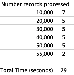
We can see, for the data set being used in this test case the optimal setting needs to be around 1,500.
What if we set the parameter to be very large? That would no necessarily make it quicker. You can see from the first table the timing starts to increase for the last two settings. There is an overhead in gathering and sending the data.
Here is a subset of the Golang code I used to perform the tests.
var currentTime = time.Now()

var i int

var custId int

arrayOne := [11] int{5, 10, 30, 50, 100, 200, 500, 1000, 1500, 2000, 2500}


currentTime = time.Now()


fmt.Println("Array Size = ", arraySize, " : ", currentTime.Format("03:04:05:06 PM"))


for index, arraySize := range arrayOne {

    currentTime = time.Now()

    fmt.Println(index, " Array Size = ", arraySize, " : ", currentTime.Format("03:04:05:06 PM"))


    db, err := sql.Open("goracle", username+"/"+password+"@"+host+"/"+database)

    if err != nil {

        fmt.Println("... DB Setup Failed")

        fmt.Println(err)

        return

    }

    defer db.Close()


    if err = db.Ping(); err != nil {

        fmt.Printf("Error connecting to the database: %s\n", err)

        return

    }


    currentTime = time.Now()

    fmt.Println("...Executing Query", currentTime.Format("03:04:05:06 PM"))

    dbQuery := "select cust_id from sh.customers"

    rows, err := db.Query(dbQuery, goracle.FetchRowCount(arraySize))

    if err != nil {

        fmt.Println(".....Error processing query")

        fmt.Println(err)

        return

    }

    defer rows.Close()


    i = 0

    currentTime = time.Now()

    fmt.Println("... Parsing query results", currentTime.Format("03:04:05:06 PM"))

   for rows.Next() {

        rows.Scan(&custId)

        i++

        if i% 10000 == 0 {

            currentTime = time.Now()

            fmt.Println("...... ",i, " customers processed", currentTime.Format("03:04:05:06 PM"))

        }

    }


    currentTime = time.Now()

    fmt.Println(i, " customers processed", currentTime.Format("03:04:05:06 PM"))


    fmt.Println("... Closing connection")

    finishTime := time.Now()

    fmt.Println("Finished at ", finishTime.Format("03:04:05:06 PM"))


}
Auto enabling APPROX_* function in the Oracle Database
With the releases of 12.1 and 12.2 of Oracle Database we have seen some new functions that perform approximate calculations. These include:
- APPROX_COUNT_DISTINCT
- APPROX_COUNT_DISTINCT_DETAIL
- APPROX_COUNT_DISTINCT_AGG
- APPROX_MEDIAN
- APPROX_PERCENTILE
- APPROX_PERCENTILE_DETAIL
- APPROX_PERCENTILE_AGG
These functions can be used when approximate answers can be used instead of the exact answer. Yes can have many scenarios for these and particularly as we move into the big data world, the ability to process our data quickly is slightly more important and exact numbers. For example, is there really a difference between 40% of our customers being of type X versus 41%. The real answer to this is, ‘It Depends!’, but for a lot of analytical and advanced analytical methods this difference doesn’t really make a difference.
There are various reports of performance improvement of anything from 6x to 50x with the response times of the queries that are using these functions, instead of using the more traditional functions.
If you are a BI or big data analyst and you have build lots of code and queries using the more traditional functions. But what if you now want to use the newer functions. Does this mean you have go and modify all the code you have written over the years? you can imagine getting approval to do this!
The simple answer to this question is ‘No’. No you don’t have to change any code, but with some parameter changes for the DB or your session you can tell the database to automatically switch from using the traditional functions (count, etc) to the newer more optimised and significantly faster APPROX_* functions.
So how can you do this magic?
First let us see what the current settings values are:
SELECT name, value
FROM   v$ses_optimizer_env
WHERE  sid = sys_context('USERENV','SID')
AND    name like '%approx%';

Now let us run a query to test what happens using the default settings (on a table I have with 10,500 records).
set auto trace on

select count(distinct cust_id) from test_inmemory;

COUNT(DISTINCTCUST_ID)
----------------------
		  1500


Execution Plan
----------------------------------------------------------
Plan hash value: 2131129625

--------------------------------------------------------------------------------------
| Id  | Operation	     | Name	     | Rows  | Bytes | Cost (%CPU)| Time     |
--------------------------------------------------------------------------------------
|   0 | SELECT STATEMENT     |		     |	   1 |	  13 |	  70   (2)| 00:00:01 |
|   1 |  SORT AGGREGATE      |		     |	   1 |	  13 |		  |	     |
|   2 |   VIEW		     | VW_DAG_0      |	1500 | 19500 |	  70   (2)| 00:00:01 |
|   3 |    HASH GROUP BY     |		     |	1500 |	7500 |	  70   (2)| 00:00:01 |
|   4 |     TABLE ACCESS FULL| TEST_INMEMORY | 10500 | 52500 |	  69   (0)| 00:00:01 |
--------------------------------------------------------------------------------------
Let us now set the automatic usage of the APPROX_* function.
alter session set approx_for_aggregation = TRUE;

SQL> select count(distinct cust_id) from test_inmemory;

COUNT(DISTINCTCUST_ID)
----------------------
		  1495


Execution Plan
----------------------------------------------------------
Plan hash value: 1029766195

---------------------------------------------------------------------------------------
| Id  | Operation	      | Name	      | Rows  | Bytes | Cost (%CPU)| Time     |
---------------------------------------------------------------------------------------
|   0 | SELECT STATEMENT      | 	      |     1 |     5 |    69	(0)| 00:00:01 |
|   1 |  SORT AGGREGATE APPROX| 	      |     1 |     5 | 	   |	      |
|   2 |   TABLE ACCESS FULL   | TEST_INMEMORY | 10500 | 52500 |    69	(0)| 00:00:01 |
---------------------------------------------------------------------------------------
We can see above that the APPROX_* equivalent function was used, and slightly less work. But we only used this on a very small table.
The full list of session level settings is:
alter session set approx_for_aggregation = TRUE;
alter session set approx_for_aggregation = FALSE;

alter session set approx_for_count_distinct = TRUE;
alter session set approx_for_count_distinct = FALSE;

alter session set approx_for_percentile = 'PERCENTILE_CONT DETERMINISTIC';
alter session set approx_for_percentile = PERCENTILE_DISC;
alter session set approx_for_percentile = NONE;
Or at a system wide level:
alter system set approx_for_aggregation = TRUE;
alter system set approx_for_aggregation = FALSE;

alter system set approx_for_count_distinct = TRUE;
alter system set approx_for_count_distinct = FALSE;

alter system set approx_for_percentile = 'PERCENTILE_CONT DETERMINISTIC';
alter system set approx_for_percentile = PERCENTILE_DISC;
alter system set approx_for_percentile = NONE;
And to reset back to the default settings:
alter system reset approx_for_aggregation;
alter system reset approx_for_count_distinct;
alter system reset approx_for_percentile;

You must be logged in to post a comment.