
21c
Oracle on AWS costs
In a previous post I walked through the steps of setting up an Oracle Database on AWS RDS. It was a very simple and straight forward process. The only thing to watch out for was to open the network to allow traffic in and out. I also showed how to connect SQL Developer to that database.
I’ve been using it for a few days and needed to move onto other things for a few days. I could leave the Database up and running during this period or I could shut down the Database to save a few dollars/euro. It also gave me a chance to see how much this database cloud instance is costing me. In my previous post, it was estimated to cost about 0.89c per day.
Before we look at the Actual/Real costs, let’s walk through the steps of shutting down the database.
To stop the database, click on the Actions button on the top right hand side of the screen, just above the database summary details. You will get a confirmation window/box appearing, see image below, asking you to confirm by clicking ‘Yes, Stop Now’.
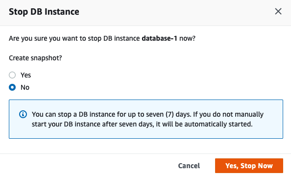
It will take a few minutes for this shutdown to complete and in my case it took approx. 8 minutes, which was a little surprising as no one was using it at the time. You might need to refresh the webpage to see this change.

That’s all very simple, but it does give you a warning about the stopped database instance. It will be restarted in 7 days time! So if this is a database you will occasionally use, then you will need to carefully manage this particular feature, otherwise you will end up with the database automatically starting and you will be paying for this.
What about the Costs?
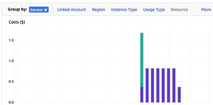
The costs for running this service can be found in the AWS Cost Management page. Here we can see the database was running for 7 and a bit days before I shut it down, and we can see the daily cost was 0.82c. Two things note about these costs. There was larger cost for the first day. Most of this cost was associated with the setup and configuration of the database service. The second thing to note is the costs listed in this console do not include taxes.
A got the bill for this usage, and it came to $6.94, consisting of $5.64 for usage (approx. 75c per day) and $1.30 in taxes/vat. Not a lot considering some cloud services, but comes out at approx 92.5c per day, which is a little more than the estimated cost when the service was being created. A small example of what can happen between the “in theory” cost of cloud versus the actual costs.
AWS RDS Oracle setup
There are lots of options available to you for creating and using an Oracle Database.
One of these options is to use AWS RDS services to create and host a Database.
Warning: Using AWS is a paid service and the RDS options are available based on the size of the server you pick. The example show in below will cost approx 89c per day or $27 per month. For this the database will be running 24×7. You could reduce this cost significantly by only starting/stopping the Database when you need it, or alternatively create an AWS lamda function service to start/stop.
First thing you need to do is go create an AWS account, and yes you will need to hand over your credit card number.
After creating your account and you have logged in, search for RDS and you will get the following display. Click on the orange button at the top of the page to Create Database.

Then select
- Standard create
- Oracle
- Architecture settings -> Use multitenant architecture
- Oracle Enterprise Edition
- Version -> use the drop down and select latest version (in my case 21)
- Templates -> Dev/Test
- Instance Identifier -> database-1
- Master Username -> admin
- Master password -> <set password> and confirm it
- DB Instance Class – as we only want a DB for playing with, go with the cheapest -> db.t3.small (Hint: Scroll to bottom of page to see the estimated monthly costs)
- Storage type -> General Purpose SSD. If you change this to Magnetic, you will see the cost drop by approx $2 per month. I selected General Purpose SSD
- Allocated Storage -> I set this to 20G (it’s just a small play DB)
- Disable/un-tick – Entable Storage Autoscaling
- Select defaults for VPC (Virtual Private Cloud) – see notes later on opening this to allow connection from your computer.
- Public Access – Set to Yes
- Defaults for remaining options.
[Note: You might be prompted to enter a DB Name. Keep this short, with no special characters.]
Click on ‘Create Database’ button at bottom of screen to create the database. It can take anything from a couple of minutes to 30 minutes to create the Database.
When everything is create, and you try to connect to the Database using SQL Developer, you will not be able to connect. The VPC needs to be opened to outside traffic. Click on the VPC Security Groups link, then click on the Security Group link on the next page
Then click on the ‘Edit Inbound rules’ button, and then on the ‘Add Rule’ button (bottom left) to add a new rule. Then select ‘All Traffic’ from drop down, and 0.0.0.0/0 in the Source field. Then save the rules.

You are now ready to create a connection using SQL Developer. To do this you will need database Endpoint from the RDS dashboard. You will also need the DB Name. This can be found by clicking on the ‘Configuration’ tab, and is listed on left-hand side under DB Name
Now in SQL Developer enter those details and click Test button to see if the connection works. It should! but if it doesn’t then double check the username and password, the other details entered, and the network changes made above are correct.

You can now connect and start using the Database.
Warning: You will be connecting as the ADMIN for the Database. You should never use this account for any development work. So go create a new database user/schema and use it for all your work.
Using SQL to create some festive Christmas Trees
Here are a few examples I found on the “great internet” of how SQL can be used to create some festive Christmas cheer and fun. See links to the original posts. Most of the examples shown below have been run on Oracle 21c Docker image, or on SQL Server or MySQL.
Our first example comes from Gerald Venzi who posted this on twitter. See later in the post for Christmas trees created using similar SQL queries.
WITH tree(lev, xmas) AS (
   SELECT 1 lev, RPAD(' ', 10, ' ') || '*' xmas
   FROM dual
   UNION ALL
   SELECT tree.lev+1,
          RPAD(' ', 10-tree.lev, ' ') ||
             RPAD('^', tree.lev+1, '^') ||
             LPAD('^', tree.lev, '^')  xmas
   FROM tree
   WHERE tree.lev < 10
)
SELECT '    Merry Christmas!' AS "Merry Christmas!" FROM dual
UNION ALL
SELECT xmas FROM TREE
UNION ALL
SELECT '         | |' FROM dual
UNION ALL
SELECT '      ~~/   \~~' FROM dual;
Our next example includes using Spatial Data on SQL Server to create a Christmas Tree. This example comes from Niket Kedia.
USE tempdb
GO

— Create a table

CREATE TABLE #xmasTREE (shape GEOMETRY )

–Creating the Christmas tree with stars

INSERT INTO #xmasTREE

VALUES
(‘POLYGON((4 0, 0 0, 4 2, 1 2, 4 4, 1 4, 4 6, 2 6, 5 10, 8 6, 6 6, 9 4, 6 4, 9 2, 6 2, 10 0, 4 0))’ ),
(‘POLYGON((3.5 0, 4 -1, 6 -1, 6.5 0, 3.5 0))’ ),
(‘POLYGON((5 9.5, 4.5 9.25, 4.6 9.9, 4.1 10.2, 4.8 10.2, 5 10.9, 5.2 10.2, 5.9 10.2, 5.4 9.9, 5.5 9.25, 5 9.5))’ ),
(‘POLYGON((2 5.5, 1.5 5.25, 1.6 5.9, 1.1 6.2, 1.8 6.2, 2 6.9, 2.2 6.2, 2.9 6.2, 2.4 5.9, 2.5 5.25, 2 5.5))’ ),
(‘POLYGON((8 5.5, 7.5 5.25, 7.6 5.9, 7.1 6.2, 7.8 6.2, 8 6.9, 8.2 6.2, 8.9 6.2, 8.4 5.9, 8.5 5.25, 8 5.5))’ ),
(‘POLYGON((1 3.5, 0.5 3.25, 0.6 3.9, 0.1 4.2, 0.8 4.2, 1 4.9, 1.2 4.2, 1.9 4.2, 1.4 3.9, 1.5 3.25, 1 3.5))’ ),
(‘POLYGON((9 3.5, 8.5 3.25, 8.6 3.9, 8.1 4.2, 8.8 4.2, 9 4.9, 9.2 4.2, 9.9 4.2, 9.4 3.9, 9.5 3.25, 9 3.5))’ ), (‘POLYGON((1 1.5, 0.5 1.25, 0.6 1.9, 0.1 2.2, 0.8 2.2, 1 2.9, 1.2 2.2, 1.9 2.2, 1.4 1.9, 1.5 1.25, 1 1.5))’ ), (‘POLYGON((9 1.5, 8.5 1.25, 8.6 1.9, 8.1 2.2, 8.8 2.2, 9 2.9, 9.2 2.2, 9.9 2.2, 9.4 1.9, 9.5 1.25, 9 1.5))’ ),
(‘POLYGON((0 -0.5, -0.5 -0.75, -0.4 -0.1, -0.9 0.2, -0.2 0.2, 0 0.9, 0.2 0.2, 0.9 0.2, 0.4 -0.1, 0.5 -0.75, 0 -0.5))’ ),
(‘POLYGON((10 -0.5, 9.5 -0.75, 9.6 -0.1, 9.1 0.2, 9.8 0.2, 10 0.9, 10.2 0.2, 10.9 0.2, 10.4 -0.1, 10.5 -0.75, 10 -0.5))’ ),
(‘POLYGON((5 -2, 4.5 -2, 4.5 -1, 5 -1, 5.5 -1, 5.5 -2, 5 -2))’)

–Create the “Merry Christmas” greetings

INSERT INTO #xmasTREE

VALUES (‘POLYGON((-2 11, -2 12, -1.75 12, -1.5 11.5, -1.25 12, -1 12, -1 11, -1.25 11, -1.25 11.7, -1.5 11.2, -1.75 11.7, -1.75 11, -2 11))’ ),–M
(‘POLYGON((-1 11, -1 12, 0 12, 0 11.8, -0.75 11.8, -0.75 11.6, -0.25 11.6, -0.25 11.4, -0.75 11.4, -0.75 11.2, 0 11.2, 0 11, -1 11))’ ),–E
(‘POLYGON((0 11, 0 12, 1 12, 1 11.5, 0.4 11.5, 1 11, 0.7 11, 0.2 11.4, 0.2 11, 0 11),(0.2 11.8, 0.8 11.8, 0.8 11.7, 0.2 11.7, 0.2 11.8))’ ),–R
(‘POLYGON((1 11, 1 12, 2 12, 2 11.5, 1.4 11.5, 2 11, 1.7 11, 1.2 11.4, 1.2 11, 1 11),(1.2 11.8, 1.8 11.8, 1.8 11.7, 1.2 11.7, 1.2 11.8))’ ),–R
(‘POLYGON((2 12, 2.2 12, 2.5 11.6, 2.8 12, 3 12, 2.6 11.5, 2.6 11, 2.4 11, 2.4 11.5, 2 12))’ ), –Y
(‘POLYGON((4 11, 4 12, 5 12, 5 11.8, 4.25 11.8, 4.25 11.2, 5 11.2, 5 11, 4 11))’ ),–C
(‘POLYGON((5 11, 5 12, 5.2 12, 5.2 11.6, 5.8 11.6, 5.8 12, 6 12, 6 11, 5.8 11, 5.8 11.4, 5.2 11.4, 5.2 11, 5 11))’ ),–H
(‘POLYGON((6 11, 6 12, 7 12, 7 11.5, 6.4 11.5, 7 11, 6.7 11, 6.2 11.4, 6.2 11, 6 11),(6.2 11.8, 6.8 11.8, 6.8 11.7, 6.2 11.7, 6.2 11.8))’ ),–R
(‘POLYGON((7.2 11, 7.2 11.2, 7.4 11.2, 7.4 11.8, 7.2 11.8, 7.2 12, 7.8 12, 7.8 11.8, 7.6 11.8, 7.6 11.2, 7.8 11.2, 7.8 11, 7.2 11))’ ),–I
(‘POLYGON((8 11, 8 11.2, 8.8 11.2, 8.8 11.4, 8 11.4, 8 12, 9 12, 9 11.8, 8.2 11.8, 8.2 11.6, 9 11.6, 9 11, 8 11))’ ),–S
(‘POLYGON((9 11.8, 9 12, 10 12, 10 11.8, 9.6 11.8, 9.6 11, 9.4 11, 9.4 11.8, 9 11.8))’ ),–T
(‘POLYGON((10 11, 10 12, 10.25 12, 10.5 11.5, 10.75 12, 11 12, 11 11, 10.75 11, 10.75 11.7, 10.5 11.2, 10.25 11.7, 10.25 11, 10 11))’ ),–M
(‘POLYGON((11 11, 11 12, 12 12, 12 11, 11.75 11, 11.75 11.3, 11.25 11.3, 11.25 11, 11 11),(11.25 11.5, 11.25 11.8, 11.75 11.8, 11.75 11.5, 11.25 11.5))’ ),–A
(‘POLYGON((12 11, 12 11.2, 12.8 11.2, 12.8 11.4, 12 11.4, 12 12, 13 12, 13 11.8, 12.2 11.8, 12.2 11.6, 13 11.6, 13 11, 12 11))’ )–S

–Decorate the tree with some round bell circles

DECLARE @counter INT = 0

,@x INT

,@y INT ;

WHILE ( @counter < 25 )

BEGIN

INSERT INTO #xmasTREE

VALUES (GEOMETRY::Point(RAND() * 5 + 2.5, RAND() * 8.5, 0).STBuffer(0.3) )

SET @counter+=1 ;

END

Select * from #xmasTREE
Drop table #xmasTREE
Our next example comes from StackOverflow with a similar example for MySQL.
DECLARE @g TABLE (g GEOMETRY, ID INT IDENTITY(1,1));


-- Adjust Color

INSERT INTO @g(g) SELECT TOP 29 CAST('POLYGON((0 0, 0 0.0000001, 0.0000001 0.0000001, 0 0))' as geometry) FROM sys.messages;

-- Build Christmas Tree

INSERT INTO @g(g) VALUES (CAST('POLYGON((0 0,900 0,450 400, 0 0 ))' as geometry).STUnion(CAST('POLYGON((80 330,820 330,450 640,80 330 ))' as geometry)).STUnion(CAST('POLYGON((210 590,690 590,450 800, 210 590 ))' as geometry)));

-- Adjust Color

INSERT INTO @g(g) SELECT TOP 294 CAST('POLYGON((0 0, 0 0.0000001, 0.0000001 0.0000001, 0 0))' as geometry) FROM sys.messages;

-- Build a Star

INSERT INTO @g(g) VALUES (CAST('POLYGON ((450 910, 465.716 861.631, 516.574 861.631, 475.429 831.738, 491.145 783.369, 450 813.262, 408.855 783.369, 424.571 831.738, 383.426 861.631, 434.284 861.631, 450 910))' as geometry));

-- Build Colored Balls

INSERT INTO @g(g) SELECT TOP 2 CAST('POLYGON((0 0, 0 0.0000001, 0.0000001 0.0000001, 0 0))' as geometry) FROM sys.messages;

INSERT INTO @g(g) VALUES (CAST('CURVEPOLYGON (CIRCULARSTRING (80 290, 110 320, 140 290, 110 260, 80 290))' as geometry));

INSERT INTO @g(g) SELECT TOP 2 CAST('POLYGON((0 0, 0 0.0000001, 0.0000001 0.0000001, 0 0))' as geometry) FROM sys.messages;

INSERT INTO @g(g) VALUES (CAST('CURVEPOLYGON (CIRCULARSTRING (760 290, 790 320, 820 290, 790 260, 760 290))' as geometry));

INSERT INTO @g(g) SELECT TOP 3 CAST('POLYGON((0 0, 0 0.0000001, 0.0000001 0.0000001, 0 0))' as geometry) FROM sys.messages;

INSERT INTO @g(g) VALUES (CAST('CURVEPOLYGON (CIRCULARSTRING (210 550, 240 580, 270 550, 240 520, 210 550))' as geometry));

INSERT INTO @g(g) SELECT TOP 46 CAST('POLYGON((0 0, 0 0.0000001, 0.0000001 0.0000001, 0 0))' as geometry) FROM sys.messages;

INSERT INTO @g(g) VALUES (CAST('CURVEPOLYGON (CIRCULARSTRING (630 550, 660 580, 690 550, 660 520, 630 550))' as geometry));


SELECT g FROM @g ORDER BY ID;

GO
Connor McDonold posted the following SQL to create a Christmas Tree on StackOverflow in 2020, and wrote a blog post for it in December 2021. I just made one very very minor change to it.
You need to be careful where you run this. It runs best on/in a Linux environment, docker, VM, etc using SQL Command Line or SQL*Plus. For me, SQL Developer struggled to present the results correctly.
select replace(replace(replace(r,'X',chr(27)||'[42m'||chr(27)||'[1;'||to_char(32)||'m'||'X'||chr(27)||'[0m'),
    'T',chr(27)||'[43m'||chr(27)||'[1;'||to_char(33)||'m'||'T'||chr(27)||'[0m'),
    '@',chr(27)||'[33m'||chr(27)||'[1;'||to_char(31)||'m'||'@'||chr(27)||'[0m')  Happy_Christmas
from ( select lpad(' ',20-e-i)|| case when dbms_random.value < 0.3 then substr(s,1,e*2-3+i*2)
       else substr(substr(s,1,dbms_random.value(1,e*2-3+i*2-1))||'@'||s,1,e*2-3+i*2) end r
from ( select rpad('X',40,'X') s,rpad('T',40,'T') t from dual ) ,
( select level i, level+2 hop from dual connect by level <= 4 ) , lateral
( select level e from dual connect by level <= hop ) union all select lpad(' ',17)||substr(t,1,3)
from ( select rpad('X',40,'X') s,rpad('T',40,'T') t from dual ) connect by level <= 5 );
Next up we have a simpler Christmas Tree. This comes from Matheus Boesing and his original post on grepora.
clear screen
set feedback off;
set heading off;
set pages 80;
SELECT DECODE(SIGN(FLOOR(maxwidth / 2) - ROWNUM),
              1,
              LPAD(' ', FLOOR(maxwidth / 2) - (ROWNUM - 1)) ||
              RPAD('*', 2 * (ROWNUM - 1) + 1, ' *'),
              LPAD('* * *', FLOOR(maxwidth / 2) + 3))
  FROM all_objects, (SELECT 40 AS maxwidth FROM DUAL)
 WHERE ROWNUM < FLOOR(maxwidth / 2) + 5
union all select '     Happy Christmas from Brendan!' from dual;
set heading on;
set feedback on;
This next example comes from LearnSQL and is similar to the previous example, but this time we get a multiple trees.
clear screen
set feedback off;
set heading off;
set pages 80;
WITH small_tree(tree_depth,pine) AS (
  SELECT 1 tree_depth,
  rpad(' ',10,' ') || '*'
  || rpad(' ',20,' ') || '*'
  || rpad(' ',20,' ') || '*'
  pine
  FROM   dual
  UNION ALL
  SELECT small_tree.tree_depth +1 tree_depth,
  rpad(' ',10-small_tree.tree_depth,' ') || rpad('*',small_tree.tree_depth+1,'.') || lpad('*',small_tree.tree_depth,'.')
  || rpad(' ',20-small_tree.tree_depth-tree_depth,' ') || rpad('*',small_tree.tree_depth+1,'.') || lpad('*',small_tree.tree_depth,'.')
  || rpad(' ',20-small_tree.tree_depth-tree_depth,' ') || rpad('*',small_tree.tree_depth+1,'.') || lpad('*',small_tree.tree_depth,'.') pine
  FROM   small_tree
  where small_tree.tree_depth < 10
)
SELECT   rpad(' ',9,' ') ||'Ho'
         || rpad(' ',19,' ') || 'Ho'
         || rpad(' ',19,' ') || 'Ho'
  pine
  FROM   dual
  UNION ALL
SELECT pine
FROM small_tree;
set heading on;
set feedback on;
Hans Viehmann from the Oracle Spatial teams sent me this example using Oracle Spatial and Oracle Spatial Studio. The geospatial data is defined using GeoJSON. The funny coordinates are referencing the Santa Claus village near Rovaniemi in Finnish Lappland, right on the Arctic Circle. Oracle Spatial Studio can be used to view the Christmas tree on a map (see image below).
DROP TABLE XMAS_TREE_JSON;

DROP TABLE XMAS_TREE;

CREATE TABLE XMAS_TREE_JSON (
    ID   NUMBER(10),
    DATA CLOB,
    CONSTRAINT XMAS_TREE_PK PRIMARY KEY ( ID ),
    CONSTRAINT XMAS_TREE_JSON_CHK CHECK ( DATA IS JSON )
);

INSERT INTO XMAS_TREE_JSON VALUES (
    1,
    '{
      "type": "Feature",
      "properties": { "label": "Tree"},
      "geometry": {
        "type": "Polygon",
        "coordinates": [
          [[25.84725335240364,
              66.5437744044363],
            [25.847166180610653,
              66.543721555766],
            [25.847235918045044,
              66.5437231572425],
            [25.84712728857994,
              66.5436740452493],
            [25.84722116589546,
              66.54367564672889],
            [25.847095102071762,
              66.54362012871027],
            [25.847205072641373,
              66.54362226402098],
            [25.847202390432358,
              66.54361105363778],
            [25.847297608852386,
              66.54361212129352],
            [25.847297608852386,
              66.5436238655039],
            [25.84740623831749,
              66.5436243993315],
            [25.84728017449379,
              66.54367724820834],
            [25.84736466407776,
              66.54367724820834],
            [25.847273468971252,
              66.54372369106797],
            [25.847321748733517,
              66.54372369106797],
            [25.84725335240364,
              66.5437744044363]
          ]
        ]
      }
    }'
);

COMMIT;

CREATE TABLE XMAS_TREE
    AS
        SELECT
            ID,
            JSON_VALUE(DATA, '$.geometry' RETURNING SDO_GEOMETRY) AS SHAPE,
            JSON_VALUE(DATA, '$.properties.label')                AS LABEL
        FROM
            XMAS_TREE_JSON;
Happy Christmas everyone.
Working with External Data on Oracle DB Docker
With multi-modal databases (such as Oracle and many more) you will typically work with data in different formats and for different purposes. One such data format is with data located external to the database. The data will exist in files on the operating systems on the DB server or on some connected storage device.
The following demonstrates how to move data to an Oracle Database Docker image and access this data using External Tables. (This based on an example from Oracle-base.com with a few additional commands).
For this example, I’ll be using an Oracle 21c Docker image setup previously. Similarly the same steps can be followed for the 18c XE Docker image, by changing the Contain Id from 21cFull to 18XE.
Step 1 – Connect to OS in the Docker Container & Create Directory
The first step involves connecting the the OS of the container. As the container is setup for default user ‘oracle’, that is who we will connect as, and it is this Linux user who owns all the Oracle installation and associated files and directories
docker exec -it 21cFull /bin/bash
When connected we are in the Home directory for the Oracle user.
The Home directory contains lots of directories which contain all the files necessary for running the Oracle Database.
Next we need to create a directory which will story the files.
mkdir ext_data
As we are logged in as the oracle Linux user, we don’t have to make any permissions changes, as Oracle Database requires read and write access to this directory.
Step 3 – Upload files to Directory on Docker container
Open another terminal window on your computer (desktop/laptop). You should have two such terminal windows open. One you opened for Step 1 above, and this one. This will allow you to easily switch between files on your computer and the files in the Docker container.
Download the two Countries files, to your computer, which are listed on Oracle-base.com. Countries1.txt and Countries2.txt.
Now you need to upload those files to the Docker container.
docker cp Countries1.txt 21cFull:/opt/oracle/ext_data/Countries1.txt
docker cp Countries2.txt 21cFull:/opt/oracle/ext_data/Countries2.txt
Step 4 – Connect to System (DBA) schema, Create User, Create Directory, Grant access to Directory
If you a new to the Database container, you don’t have any general users/schemas created. You should create one, as you shouldn’t use the System (or DBA) user for any development work. To create a new database user connect to System.
sqlplus system/SysPassword1@//localhost/XEPDB1
To use sqlplus command line tool you will need to install Oracle Instant Client and then SQLPlus (which is a separate download from the same directory for your OS)
To create a new user/schema in the database you can run the following (change the username and password to something more sensible).
create user brendan identified by BtPassword1
default tablespace users
temporary tablespace temp;
grant connect, resource to brendan;
alter user brendan
quota unlimited on users;
Now create the Directory object in the database, which points to the directory on the Docker OS we created in the Step 1 above. Grant ‘brendan’ user/schema read and write access to this Directory
CREATE OR REPLACE DIRECTORY ext_tab_data AS '/opt/oracle/ext_data';
grant read, write on directory ext_tab_data to brendan;
Now, connect to the brendan user/schema.
Step 5 – Create external table and test
To connect to brendan user/schema, you can run the following if you are still using SQLPlus
SQL> connect brendan/BtPassword1@//localhost/XEPDB1
or if you exited it, just run this from the command line
sqlplus system/SysPassword1@//localhost/XEPDB1
Create the External Table (same code from oracle-base.com)
CREATE TABLE countries_ext (
  country_code      VARCHAR2(5),
  country_name      VARCHAR2(50),
  country_language  VARCHAR2(50)
)
ORGANIZATION EXTERNAL (
  TYPE ORACLE_LOADER
  DEFAULT DIRECTORY ext_tab_data
  ACCESS PARAMETERS (
    RECORDS DELIMITED BY NEWLINE
    FIELDS TERMINATED BY ','
    MISSING FIELD VALUES ARE NULL
    (
      country_code      CHAR(5),
      country_name      CHAR(50),
      country_language  CHAR(50)
    )
  )
  LOCATION ('Countries1.txt','Countries2.txt')
)
PARALLEL 5
REJECT LIMIT UNLIMITED;
It should create for you. If not and you get an error then if will be down to a typo on directory name or the files are not in the directory or something like that.
We can now query the External Table as if it is a Table in the database.
SQL> set linesize 120
SQL> select * from countries_ext order by country_name;
COUNT COUNTRY_NAME                         COUNTRY_LANGUAGE
----- ------------------------------------ ------------------------------
ENG   England                              English
FRA   France                               French
GER   Germany                              German
IRE   Ireland                              English
SCO   Scotland                             English
USA   Unites States of America             English
WAL   Wales                                Welsh

7 rows selected.
All done!
Oracle 21c XE Database and Docker setup
You know when you are waiting for the 39 bus for ages, and then two of them turn up at the same time. It’s a bit like this with Oracle 21c XE Database Docker image being released a few days after the 18XE Docker image!
Again we have Gerald Venzi to thank for putting these together and making them available.
23c Database – If you want to use the 23c Database, Check out this post for the command to install
Are you running an Apple M1 chip Laptop? If so, follow these instructions (and ignore the rest of this post)
If you want to install Oracle 21c XE yourself then go to the download page and within a few minutes you are ready to go. Remember 21c XE is a fully featured version of their main Enterprise Database, with a few limitations, basically on size of deployment. You’d be surprised how many organisations who’s data would easily fit within these limitations/restrictions. The resource limits of Oracle Database 21 XE include:
- 2 CPU threads
- 2 GB of RAM
- 12GB of user data (Compression is included so you can store way way more than 12G)
- 3 pluggable Databases
It is important to note, there are some additional restrictions on feature availability, for example Parallel Query is not possible, etc.
Remember the 39 bus scenario I mentioned above. A couple of weeks ago the Oracle 18c XE Docker image was released. This is a full installation of the database and all you need to do is to download it and run it. Nothing else is required. Check out my previous post on this.
To download, install and run Oracle 21c XE Docker image, just run the following commands.
docker pull gvenzl/oracle-xe:21-full

docker run -d -p 1521:1521 -e ORACLE_PASSWORD=SysPassword1 -v oracle-volume:/opt/oracle/XE21CFULL/oradata gvenzl/oracle-xe:21-full

docker rename da37a77bb436 21cFull

sqlplus system/SysPassword1@//localhost/XEPDB1
It’s a good idea to create a new schema for your work. Here is an example to create a schema called ‘demo’. First log into system using sqlplus, as shown above, and then run these commands.
create user demo identified by demo quota unlimited on users;
grant connect, resource to demo;
To check that schema was created you can connect to it using sqlplus.
connect demo/demo@//localhost/XEPDB1
Then to stop the image from running and to restart it, just run the following
docker stop 21cFull
docker start 21cFull
Check out my previous post on Oracle 18c XE setup for a few more commands.
SQL Developer Connection Setup
An alternative way to connect to the Database is to use SQL Developer. The following image shows and example of connecting to a schema called DEMO, which I created above. See the connection details in this image. They are the same as what is shown above when connecting using sqlplus.

Collection of Oracle 21c posts on new Machine Learning and Statistical functions
Oracle 21c was officially released a few days about and this post contains links to some blog posts I’ve written on new machine learning and statistical functions in the new Oracle 21c.
- Adam Optimization Solver for Neural Network Algorithm
- MSET-SPRT Algorithm
- XGBoost Algorithm
- Measuring SKEWNESS Function
- Measuring tailedness of data with KURTOSIS Function
I also have posts on new OML4Py and AutoML too, and I’ll have a different set of posts for those, so look out them.
Also check out my previous blog post that covers new machine learning feature introduced in Oracle 19c.
Measuring Kurtosis of Data in Oracle (21c)
Kurtosis is a new analytics function in Oracle 21c (20c) and is one of a set of commonly used statistical functions used to evaluate data to see and understand the behavior of the data.
[See my previous post where I give examples of the new Skewness functions]
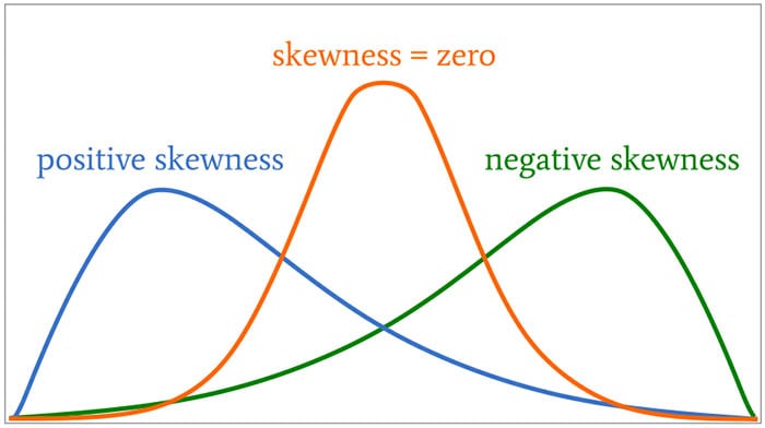
Kurtosis is the measurement of the tails of the data distribution and its comparison with that of normal distribution. The Kurtosis of the normal distribution is said to be 3. To make interpenetrating results easier (a Zero) kurtosis measure for gaussian/normal distribution by subtracting 3 from its value, this is called Excess Kurtosis. Kurtosis can be used to describe the height or the breath of the distributions, when compared to a normal distributions, although this is not theoretically correct, it gives a simpler explanation and visualization of it. The following diagram gives an example of a normal distribution, a plot of Positive Kurtosis and Negative Kurtosis.

Prior to the new Kurtosis SQL functions (KURTOSIS_POP and KURTOSIS_SAMP), you had to calculate the Kurtosis value manually using something like the following SQL. These use the same data and attributes set used for the Skewness examples.
select avg(KV) K_value
from (select power((age - avg(age) over ())/stddev(age) over (), 4) KV
      from cust_data)
union all
select avg(KV) K_value
from (select power((duration - avg(duration) over ())/stddev(duration) over (), 4) KV
      from cust_data);

K_value
------------------------------------------
3.79088571963003808388287765230733611415
23.24420570926391173498028369605428048285
These don’t include the subtraction of 3 to give a zero kurtosis, and these values can be compared to the data distribution charts shown in the Skewness post.
Now with the new Kurtosis functions it simplifies the tasks of getting these values.
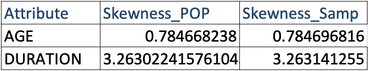
SELECT kurtosis_pop(age), kurtosis_samp(age)
FROM bank_additional
union all
SELECT kurtosis_pop(duration), kurtosis_samp(duration)
FROM bank_additional;

KURTOSIS_POP         KURTOSIS_SAMP
------------------   -----------------------------------------
 0.791069803527387    0.79131153115443467194451597661213420763
20.245334438614832   20.24793801497878942299945619307526969226
As you can see the Kurtosis function have the subtraction include.
As with the Skewness functions, the SAMP version works on a sample of the data values and as the number inputs increases, and differences between the POP and SAMP will reduce.
Measuring Skewness of Data in Oracle (21c)
When analyzing data you will look at using a variety of different statistical functions to explore variable data insights.
One of these is the Skewness of the data.
Skewness is a measure of the asymmetry of the probability distribution about its mean. This looks a the tail of the data, with a positive value indicating the tail on the right side of the distribution, and a negative value when the tail is on the left hand side. A zero value indicates the tails on both side balance out, as shown in the following image.
Most SQL dialects support Skewness using with an inbuilt function. But if it doesn’t then you would need to write your own version of the calculation, for example using the following.
SELECT avg(SV) S_value
FROM   (SELECT  power((age – avg(age) over ())/stddev(age) over (), 3) SV
        FROM    cust_data)
Here are charts illustrating the data in my table. These include the distributions for the AGE and DURATION attributes.
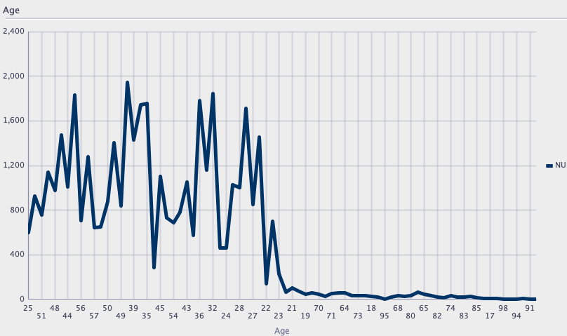

We can see the data is skewed. When we run the above code we get the following values.
Age = 0.78
Duration = 3.26
We can see the skewness of Duration is significantly longer, giving a positive value as the skewness is to the right.
In Oracle 21s we now have new Skewness functions called SKEWNESS_POP and SKEWNESS_SAMP. The POP version of the function considers all records, where as the SAMP function considers a sample of the records. When your data set grows into many millions of records the SKEWNESS_SAMP will give a quicker response as it works with a sample of the data set
Both functions will give similar values but at the number of input records the returned values will returned will converge.
SELECT skewness_pop(age), skewness_samp(age)
FROM cust_data;
SELECT skewness_pop(duration), skewness_samp(duration)
FROM cust_data;
Enhanced Window Clause functionality in Oracle 21c (20c)
Updated: Changed 20c to Oracle 21c, as Oracle 20c Database never really existed 🙂
The Oracle Database has had advanced analytical functions for some time now and with each release we get to have some new additions or some enhancements to existing functionality.
One new enhancement, available and documented in 21c (not yet released at time of writing this), is changing in the way the Window Clause can be defined for analytic functions. Oracle 21c is available on Oracle Cloud as a pre-release for evaluation purposes (but it won’t be available for much longer!). The examples shown below are based on using this 21c pre-release of the database.
NOTE: At this point, no one really knows when or if 20c will be released. I’m sure all the documented 20c new features will be rolled into 21c, whenever that will be released.
Before giving some examples of the new Window Clause functionality, lets have a quick recap on how we could use it up to now (up to 19c database). Here is a simple example of windowing the data by creating partitions based on the distinct values in DEPTNO column
select deptno,
       ename,
       job,
       salary,
       avg (salary) over (partition by DEPTNO) avg_sal
from employee
order by deptno;

Here we get to see the average salary being calculated for each window partition and being reset for the next windwo partition.
The SQL:2011 standard support the defining of the Window clause in the query block, after defining the list tables for the query. This allows us to define the window clause one and then reference this for analytic function that need it. The following example illustrate this. I’ve take the able query and altered it to have the newer syntax. I’ve highlighted the new or changed code in blue. In the analytic function, the w1 refers to the Window clause defined later, and is more in keeping with how a query is logically processed.
select deptno,
       ename,
       sal,
       sum(sal) over (w1) sum_sal
from emp
   window w1 as (partition by deptno);
As you would expect we get the same results returned.
This newer syntax is particularly useful when we have many more analytic function in our queries, and some of these are using slightly different windowing. To me it makes it easier to read and to make edits, allowing an edit to be preformed once instead of for each analytic function, and avoids any errors. But making it easier to read and understand is by far the greatest benefit. Here is another example which uses different window clauses using the previous syntax.
SELECT deptno,
       ename,
       sal,
       AVG(sal) OVER (PARTITION BY deptno ORDER BY sal) AS avg_dept_sal,
       AVG(sal) OVER (PARTITION BY deptno ) AS avg_dept_sal2,
       SUM(sal) OVER (PARTITION BY deptno ORDER BY sal desc) AS sum_dept_sal
FROM emp;
Using the newer syntax this gets transformed into the following.
SELECT deptno,
       ename,
       sal,
       AVG(sal) OVER (w1) AS avg_dept_sal,
       AVG(sal) OVER (w2) AS avg_dept_sal2,
       SUM(sal) OVER (w2) AS avg_dept_sal
FROM emp
   window w1 as (PARTITION BY deptno ORDER BY sal),
          w2 as (PARTITION BY deptno),
          w3 as (PARTITION BY deptno ORDER BY sal desc);
XGBoost in Oracle 20c
 Updated: Changed 20c to Oracle 21c, as Oracle 20c Database never really existed 🙂
Another of the new machine learning algorithms in Oracle 21c Database is called XGBoost. Most people will have come across this algorithm due to its recent popularity with winners of Kaggle competitions and other similar events.
XGBoost is an open source software library providing a gradient boosting framework in most of the commonly used data science, machine learning and software development languages. It has it’s origins back in 2014, but the first official academic publication on the algorithm was published in 2016 by Tianqi Chen and Carlos Guestrin, from the University of Washington.
The algorithm builds upon the previous work on Decision Trees, Bagging, Random Forest, Boosting and Gradient Boosting. The benefits of using these various approaches are well know, researched, developed and proven over many years. XGBoost can be used for the typical use cases of Classification including classification, regression and ranking problems. Check out the original research paper for more details of the inner workings of the algorithm.
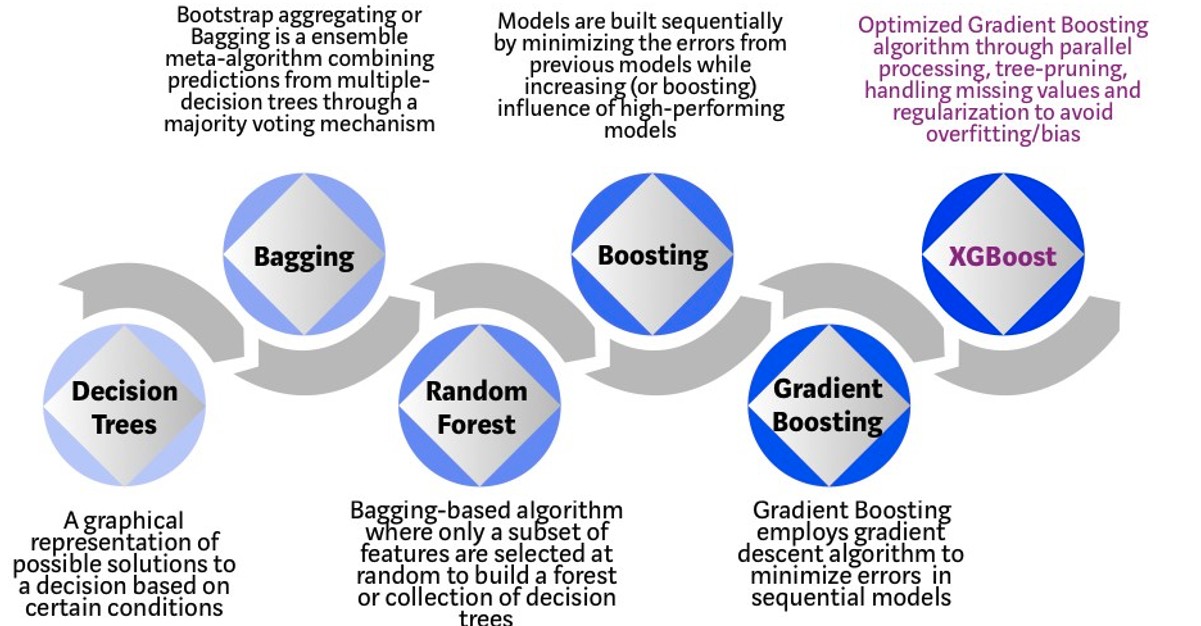
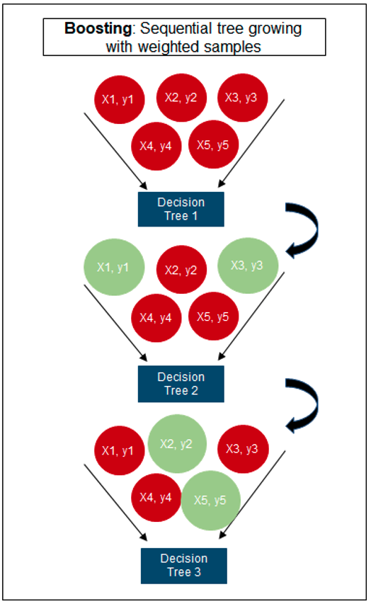
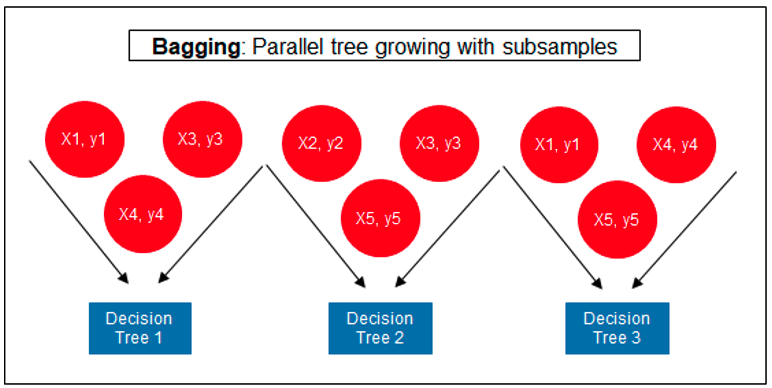
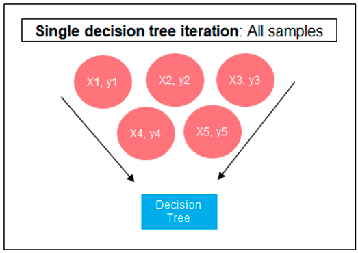
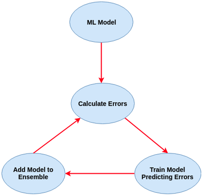 Regular machine learning models, like Decision Trees, simply train a single model using a training data set, and only this model is used for predictions. Although a Decision Tree is very simple to create (and very very quick to do so) its predictive power may not be as good as most other algorithms, despite providing model explainability. To overcome this limitation ensemble approaches can be used to create multiple Decision Trees and combines these for predictive purposes. Bagging is an approach where the predictions from multiple DT models are combined using majority voting. Building upon the bagging approach Random Forest uses different subsets of features and subsets of the training data, combining these in different ways to create a collection of DT models and presented as one model to the user. Boosting takes a more iterative approach to refining the models by building sequential models with each subsequent model is focused on minimizing the errors of the previous model. Gradient Boosting uses gradient descent algorithm to minimize errors in subsequent models. Finally with XGBoost builds upon these previous steps enabling parallel processing, tree pruning, missing data treatment, regularization and better cache, memory and hardware optimization. It’s commonly referred to as gradient boosting on steroids.
The following three images illustrates the differences between Decision Trees, Random Forest and XGBoost.
The XGBoost algorithm in Oracle 20c has over 40 different parameter settings, and with most scenarios the default settings with be fine for most scenarios. Only after creating a baseline model with the details will you look to explore making changes to these. Some of the typical settings include:
- Booster = gbtree
- #rounds for boosting = 10
- max_depth = 6
- num_parallel_tree = 1
- eval_metric = Classification error rate or RMSE for regression
As with most of the Oracle in-database machine learning algorithms, the setup and defining the parameters is really simple. Here is an example of minimum of parameter settings that needs to be defined.
BEGIN
   -- delete previous setttings
   DELETE FROM banking_xgb_settings;

   INSERT INTO BANKING_XGB_SETTINGS (setting_name, setting_value)
   VALUES (dbms_data_mining.algo_name, dbms_data_mining.algo_xgboost);

   -- For 0/1 target, choose binary:logistic as the objective.
   INSERT INTO BANKING_XGB_SETTINGS (setting_name, setting_value)
   VALUES (dbms_data_mining.xgboost_objective, 'binary:logistic’);

   commit;
END;
To create an XGBoost model run the following.


BEGIN
   DBMS_DATA_MINING.CREATE_MODEL (
      model_name          => 'BANKING_XGB_MODEL',
      mining_function     => dbms_data_mining.classification,
      data_table_name     => 'BANKING_72K',
      case_id_column_name => 'ID',
      target_column_name  => 'TARGET',
      settings_table_name => 'BANKING_XGB_SETTINGS');
END;
That’s all nice and simple, as it should be, and the new model can be called in the same manner as any of the other in-database machine learning models using functions like PREDICTION, PREDICTION_PROBABILITY, etc.
One of the interesting things I found when experimenting with XGBoost was the time it took to create the completed model. Using the default settings the following table gives the time taken, in seconds to create the model.
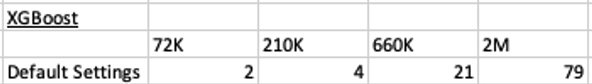
As you can see it is VERY quick even for large data sets and gives greater predictive accuracy.

You must be logged in to post a comment.