R
OML4R available on ADB
Oracle Machine Learning for R (OML4R) is available on Oracle Autonomous Database. Finally. After waiting for way, way too long we can now run R code in the Autonomous Database (in the Cloud). It’s based on using Oracle R Distribution 4.0.5 (which is based on R 4.0.5). This product was previously called Oracle R Enterprise, which I was a fan of many few years ago, so much so I wrote a book about it.
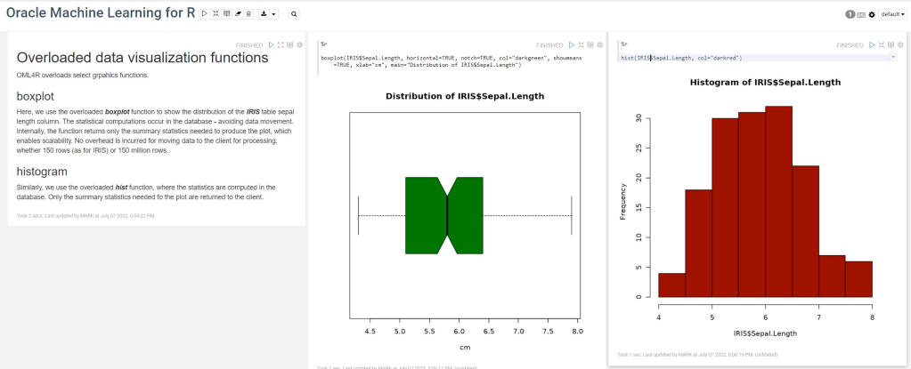
OML4R comes with all (or most) of the benefits of Oracle R Enterprise, whereby you can connect to, in this case an Oracle Autonomous Database (in the Cloud), allowing data scientists work with R code and manipulate data in the database instead of in their local environment. Embed R code in the database and enable other database users (and applications) to call this R code. Although with OML4R on ADB (in the Cloud) does come with some limitations and restrictions, which will put people/customers off from using it.
Waiting for OML4R reminds me of Eurovision Song Contest winning song by Johnny Logan titled,
I’ve been waiting such a long time
Looking out for you
But you’re not here
What’s another year
It has taken Oracle way, way too long to migrate OML4R to ADB. They’ve probably just made it available because one or two customers needed/asked it.
As the lyrics from Johnny Logan says (changing I’ve to We’ve), We’ve been waiting such a long time, most customers have moved to other languages, tools and other cloud data science platforms for their data science work. The market has moved on, many years ago.
Hopefully over the next few months, and with Oracle 23c Database, we might see some innovation, or maybe their data science and AI focus lies elsewhere within Oracle development teams.
R (ROracle) and Oracle DATE formats
When you comes to working with R to access and process your data there are a number of little features and behaviors you need to look out for.
One of these is the DATE datatype.
The main issue that you have to look for is the TIMEZONE conversion that happens then you extract the data from the database into your R environment.
There is a datatype conversions from the Oracle DATE into the POSIXct format. The POSIXct datatype also includes the timezone. But the Oracle DATE datatype does not have a Timezone part of it.
When you look into this a bit more you will see that the main issue is what Timezone your R session has. By default your R session will inherit the OS session timezone. For me here in Ireland we have the time timezone as the UK. You would time that the timezone would therefore be GMT. But this is not the case. What we have for timezone is BST (or British Standard Time) and this takes into account the day light savings time. So on the 26th May, BST is one hour ahead of GMT.
OK. Let’s have a look at a sample scenario.
The Problem
As mentioned above, when I select date of type DATE from Oracle into R, using ROracle, I end up getting a different date value than what was in the database. Similarly when I process and store the data.
The following outlines the data setup and some of the R code that was used to generate the issue/problem.
Data Set-up
Create a table that contains a DATE field and insert some records.
CREATE TABLE STAFF
(STAFF_NUMBER VARCHAR2(20),
FIRST_NAME VARCHAR2(20),
SURNAME VARCHAR2(20),
DOB DATE,
PROG_CODE VARCHAR2(6 BYTE),
PRIMARY KEY (STAFF_NUMBER));

insert into staff values (123456789, 'Brendan', 'Tierney', to_date('01/06/1975', 'DD/MM/YYYY'), 'DEPT_1');
insert into staff values (234567890, 'Sean', 'Reilly', to_date('21/10/1980', 'DD/MM/YYYY'), 'DEPT_2');
insert into staff values (345678901, 'John', 'Smith', to_date('12/03/1973', 'DD/MM/YYYY'), 'DEPT_3');
insert into staff values (456789012, 'Barry', 'Connolly', to_date('25/01/1970', 'DD/MM/YYYY'), 'DEPT_4');
You can query this data in SQL without any problems. As you can see there is no timezone element to these dates.
Selecting the data
I now establish my connection to my schema in my 12c database using ROracle. I won’t bore you with the details here of how to do it but check out point 3 on this post for some details.
When I select the data I get the following.
> res<-dbSendQuery(con, "select * from staff")
> data <- fetch(res)
> data$DOB
[1] "1975-06-01 01:00:00 BST" "1980-10-21 01:00:00 BST" "1973-03-12 00:00:00 BST"
[4] "1970-01-25 01:00:00 BST"
As you can see two things have happened to my date data when it has been extracted from Oracle. Firstly it has assigned a timezone to the data, even though there was no timezone part of the original data. Secondly it has performed some sort of timezone conversion to from GMT to BST. The difference between GMT and BTS is the day light savings time. Hence the 01:00:00 being added to the time element that was extract. This time should have been 00:00:00. You can see we have a mixture of times!
So there appears to be some difference between the R date or timezone to what is being used in Oracle.
To add to this problem I was playing around with some dates and different records. I kept on getting this scenario but I also got the following, where we have a mixture of GMT and BST times and timezones. I’m not sure why we would get this mixture.
> data$DOB
[1] "1995-01-19 00:00:00 GMT" "1965-06-20 01:00:00 BST" "1973-10-20 01:00:00 BST"
[4] "2000-12-28 00:00:00 GMT"
This is all a bit confusing and annoying. So let us look at how you can now fix this.
The Solution
Fixing the problem : Setting Session variables
What you have to do to fix this and to ensure that there is consistency between that is in Oracle and what is read out and converted into R (POSIXct) format, you need to define two R session variables. These session variables are used to ensure the consistency in the date and time conversions.
These session variables are TZ for the R session timezone setting and Oracle ORA_SDTZ setting for specifying the timezone to be used for your Oracle connections.
The trick there is that these session variables need to be set before you create your ROracle connection. The following is the R code to set these session variables.
> Sys.setenv(TZ = "GMT")

> Sys.setenv(ORA_SDTZ = "GMT")
So you really need to have some knowledge of what kind of Dates you are working with in the database and if a timezone if part of it or is important. Alternatively you could set the above variables to UDT.
Selecting the data (correctly this time)
Now when we select our data from our table in our schema we now get the following, after reconnecting or creating a new connection to your Oracle schema.
> data$DOB

[1] "1975-06-01 GMT" "1980-10-21 GMT" "1973-03-12 GMT" "1970-01-25 GMT"
Now you can see we do not have any time element to the dates and this is correct in this example. So all is good.
We can now update the data and do whatever processing we want with the data in our R script.
But what happens when we save the data back to our Oracle schema. In the following R code we will add 2 days to the DOB attribute and then create a new table in our schema to save the updated data.
> data$DOB

[1] "1975-06-01 GMT" "1980-10-21 GMT" "1973-03-12 GMT" "1970-01-25 GMT"

> data$DOB <- data$DOB + days(2)
> data$DOB
[1] "1975-06-03 GMT" "1980-10-23 GMT" "1973-03-14 GMT" "1970-01-27 GMT"
> dbWriteTable(con, "STAFF_2", data, overwrite = TRUE, row.names = FALSE)
[1] TRUE
I’ve used the R package Libridate to do the date and time processing.
When we look at this newly created table in our Oracle schema we will see that we don’t have DATA datatype for DOB, but instead it is created using a TIMESTAMP data type.
If you are working with TIMESTAMP etc type of data types (i.e. data types that have a timezone element that is part of it) then that is a slightly different problem.
PRECIS R package
If you use R then you are very familiar with the SUMMARY function.
If you use R then you are very familiar with the name Hadley Wickham. He has produced some really cool packages for R.
He has produced a new R package and function that complements the commonly used SUMMARY R function.
The following outlines how you can install this new R package from GitHub (Hadley’s GitHub is https://github.com/hadley/).
Install the R devtools package. This will allow you to download the package code from GitHub.
install.packages("devtools")
Install the package from Hadley’s GitHub repository.
devtools::install_github("hadley/precis")
Load the library.
library(precis)
The following displays information produced by the SUMMARY and the PRECIS function.
> summary(mtcars)
      mpg             cyl             disp             hp             drat             wt
 Min.   :10.40   Min.   :4.000   Min.   : 71.1   Min.   : 52.0   Min.   :2.760   Min.   :1.513
 1st Qu.:15.43   1st Qu.:4.000   1st Qu.:120.8   1st Qu.: 96.5   1st Qu.:3.080   1st Qu.:2.581
 Median :19.20   Median :6.000   Median :196.3   Median :123.0   Median :3.695   Median :3.325
 Mean   :20.09   Mean   :6.188   Mean   :230.7   Mean   :146.7   Mean   :3.597   Mean   :3.217
 3rd Qu.:22.80   3rd Qu.:8.000   3rd Qu.:326.0   3rd Qu.:180.0   3rd Qu.:3.920   3rd Qu.:3.610
 Max.   :33.90   Max.   :8.000   Max.   :472.0   Max.   :335.0   Max.   :4.930   Max.   :5.424
      qsec             vs               am              gear            carb
 Min.   :14.50   Min.   :0.0000   Min.   :0.0000   Min.   :3.000   Min.   :1.000
 1st Qu.:16.89   1st Qu.:0.0000   1st Qu.:0.0000   1st Qu.:3.000   1st Qu.:2.000
 Median :17.71   Median :0.0000   Median :0.0000   Median :4.000   Median :2.000
 Mean   :17.85   Mean   :0.4375   Mean   :0.4062   Mean   :3.688   Mean   :2.812
 3rd Qu.:18.90   3rd Qu.:1.0000   3rd Qu.:1.0000   3rd Qu.:4.000   3rd Qu.:4.000
 Max.   :22.90   Max.   :1.0000   Max.   :1.0000   Max.   :5.000   Max.   :8.000
> precis(mtcars)
# data.frame [32 x 11]
    name  type                            precis

1    mpg   dbl  10.4 [ 15.4 ( 19.2)  22.8]  33.9
2    cyl   dbl               4 (11) 6 (7) 8 (14)
3   disp   dbl  71.1 [121.0 (196.0) 334.0] 472.0
4     hp   dbl    52 [   96 (  123)   180]   335
5   drat   dbl  2.76 [ 3.08 ( 3.70)  3.92]  4.93
6     wt   dbl  1.51 [ 2.54 ( 3.32)  3.65]  5.42
7   qsec   dbl  14.5 [ 16.9 ( 17.7)  18.9]  22.9
8     vs   dbl                     0 (18) 1 (14)
9     am   dbl                     0 (19) 1 (13)
10  gear   dbl               3 (15) 4 (12) 5 (5)
11  carb   dbl     1 [    2 (    2)     4]     8
> precis(mtcars, histogram=TRUE)
# data.frame [32 x 11]
    name  type                            precis

1    mpg   dbl           10.4 ▂▁▇▃▅▅▂▂▁▁▂▂  33.9
2    cyl   dbl      4 ▅▁▁▁▁▁▁▁▁▃▁▁▁▁▁▁▁▁▁▇     8
3   disp   dbl  71.1 ▅▁▁▃▇▂▁▁▁▁▃▁▃▁▅▁▁▁▁▁▁ 472.0
4     hp   dbl          52 ▁▅▅▇▂▂▇▁▂▁▂▁▁▁▁   335
5   drat   dbl           2.76 ▂▂▇▂▁▅▇▃▂▁▁▁  4.93
6     wt   dbl  1.51 ▁▁▂▂▁▁▂▁▂▁▇▂▂▁▁▁▁▁▁▂▁  5.42
7   qsec   dbl      14.5 ▂▂▁▁▃▇▅▁▇▂▂▂▁▁▁▁▁  22.9
8     vs   dbl      0 ▇▁▁▁▁▁▁▁▁▁▁▁▁▁▁▁▁▁▁▅     1
9     am   dbl      0 ▇▁▁▁▁▁▁▁▁▁▁▁▁▁▁▁▁▁▁▅     1
10  gear   dbl      3 ▇▁▁▁▁▁▁▁▁▅▁▁▁▁▁▁▁▁▁▂     5
11  carb   dbl            1 ▅▇▁▂▁▇▁▁▁▁▁▁▁▁     8
Managing memory allocation for Oracle R Enterprise Embedded Execution
When working with Oracle R Enterprise and particularly when you are using the ORE functions that can spawn multiple R processes, on the DB Server, you need to be very aware of the amount of memory that will be consumed for each call of the ORE function.
ORE has two sets of parallel functions for running your user defined R scripts stored in the database, as part of the Embedded R Execution feature of ORE. The R functions are called ore.groupApply, ore.rowApply and ore.indexApply. When using SQL there are “rqGroupApply” and rqRowApply. (There is no SQL function equivalent of the R function ore.indexApply)
For each parallel R process that is spawned on the DB server a certain amount of memory (RAM) will be allocated to this R process. The default size of memory to be allocated can be found by using the following query.
select name, value from sys.rq_config;

NAME                                VALUE
----------------------------------- -----------------------------------
VERSION                             1.5
MIN_VSIZE                           32M
MAX_VSIZE                           4G
MIN_NSIZE                           2M
MAX_NSIZE                           20M
The memory allocation is broken out into the amount of memory allocated for Cells and NCells for each R process.
If your parallel ORE function create a large number of parallel R processes then you can see that the amount of overall memory consumed can be significant. I’ve seen a few customers who very quickly run out of memory on their DB servers. Now that is something you do not want to happen.
How can you prevent this from happening ?
There are a few things you need to keep in mind when using the parallel enabled ORE functions. The first one is, how many R processes will be spawned. For most cases this can be estimated or calculated to a high degree of accuracy. Secondly, how much memory will be used to process each of the R processes. Thirdly, how memory do you have available on the DB server. Fourthly, how many other people will be running parallel R processes at the same time?
Examining and answering each of these may look to be a relatively trivial task, but the complexity behind these can increase dramatically depending on the answer to the fourth point/question above.
To calculate the amount of memory used during the ORE user defined R script, you can use the R garbage function to calculate the memory usage at the start and at the end of the R script, and then return the calculated amount. Yes you need to add this extra code to your R script and then remove it when you have calculated the memory usage.
gc.start <- gc(reset=TRUE)
...
gc.end <- gc()
gc.used <- gc.end[,7] - gc.start[,7] # amount consumed by the processing
Using this information and the answers to the points/questions I listed above you can now look at calculating how much memory you need to allocated to the R processes. You can set this to be static for all R processes or you can use some code to allocate the amount of memory that is needed for each R process. But this starts to become messy. The following gives some examples (using R) of changing the R memory allocations in the Oracle Database. Similar commands can be issued using SQL.
> sys.rqconfigset('MIN_VSIZE', '10M') -- min heap 10MB, default 32MB
> sys.rqconfigset('MAX_VSIZE', '100M') -- max heap 100MB, default 4GB
> sys.rqconfigset('MIN_NSIZE', '500K') -- min number cons cells 500x1024, default 1M
> sys.rqconfigset('MAX_NSIZE', '2M') -- max number cons cells 2M, default 20M
Some guidelines – as with all guidelines you have to consider all the other requirements for the Database, and in reality you will have to try to find a balance between what is listed here and what is actually possible.
- Set parallel_degree_policy to MANUAL.
- Set parallel_min_servers to the number of parallel slave processes to be started when the database instances start, this avoids start up time for the R processes. This is not a problem for long running processes. But can save time with processes running for 10s seconds
- To avoid overloading the CPUs if the parallel_max_servers limit is reached, set the hidden parameter _parallel_statement_queuing to TRUE. Avoids overloading and lets processes wait.
- Set application tables and their indexes to DOP 1 to reinforce the ability of ORE to determine when to use parallelism.
Understanding the memory requirements for your ORE processes can be tricky business and can take some time to work out the right balance between what is needed by the spawned parallel R processes and everything else that is going on in the Database. There will be a lot of trial and error in working this out and it is always good to reach out for some help. If you have a similar scenario and need some help or guidance let me know.
OUG Ireland 2017 Presentation
Here are the slides from my presentation at OUG Ireland 2017. All about running R using SQL.
Formatting results from ORE script in a SELECT statement
This blog post looks at how to format the output or the returned returns from an Oracle R Enterprise (ORE), user defined R function, that is run using a SELECT statement in SQL.
Sometimes this can be a bit of a challenge to work out, but it can be relatively easy once you have figured out how to do it. The following examples works through some scenarios of different results sets from a user defined R function that is stored in the Oracle Database.
To run that user defined R function using a SELECT statement I can use one of the following ORE SQL functions.
- rqEval
- rqTableEval
- “rqGroupEval“
- rqRowEval
For simplicity we will just use the first of these ORE SQL functions to illustrate the problem and how to go about solving it. The rqEval ORE SQL function is a generate purpose function to call a user defined R script stored in the database. The function does not require any input data set and but it will return some data. You could use this to generate some dummy/test data or to find some information in the database. Here is noddy example that returns my name.
BEGIN
   --sys.rqScriptDrop('GET_NAME');
   sys.rqScriptCreate('GET_NAME',
      'function() {
         res<-data.frame("Brendan")
         res
         } ');
END;
To call this user defined R function I can use the following SQL.
select *
from table(rqEval(null,
                  'select cast(''a'' as varchar2(50))  from dual',
                  'GET_NAME') );
For text strings returned you need to cast the returned value giving a size.
If we have a numeric value being returned we can don’t have to use the cast and instead use ‘1’ as shown in the following example. This second example extends our user defined R function to return my name and a number.
BEGIN
   sys.rqScriptDrop('GET_NAME');
   sys.rqScriptCreate('GET_NAME',
      'function() {
         res<-data.frame(NAME="Brendan", YEAR=2017)
         res
         } ');
END;
To call the updated GET_NAME function we now have to process two returned columns. The first is the character string and the second is a numeric.
select *
from table(rqEval(null,
                  'select cast(''a'' as varchar2(50)) as "NAME", 1 AS YEAR  from dual',
                  'GET_NAME') );
These example illustrate how you can process character strings and numerics being returned by the user defined R script.
The key to setting up the format of the returned values is knowing the structure of the data frame being returned by the user defined R script. Once you know that the rest is (in theory) easy.
Creating and Reading SPSS and SAS data sets in R
Have you ever been faced with having to generate a data set in the format that is needed by another analytics tool? or having to generate a data set in a particular format but you don’t have the software that generates that format? For example, if you are submitting data to the FDA and other bodies, you may need to submit the data in a SAS formatted file. There are a few ways you can go about this.
One option is that you can use the Haven R package to generate your dataset in SAS and SPSS formats. But you can also read in SAS and SPSS formatted files. I have to deal with these formatted data files all the time, and it can be a challenge, but I’ve recently come across the Haven R package that has just made my life just a little bit/lots easier. Now I can easily generate SAS and SPSS formatted data sets for my data in my Oracle Database, using R and ORE. ORE we can now use the embedded feature to build the generation of these data sets into some of our end-user applications.
Let us have a look at Haven and what it can do.
Firstly there is very little if any documentation online for it. That is ok so we will have to rely on the documentation that comes with the R packages. Again there isn’t much to help and that is because the R package mainly consists of functions to Read in these data sets, functions to Write these data sets and some additional functions for preparing data.
For reading in data sets we have the following functions:
# SAS
read_sas("mtcars.sas7bdat")
# Stata
read_dta("mtcars.dta")
# SPSS
read_sav("mtcars.sav")
For writing data sets we have the following functions:
# SAS
write_sas(mtcars, "mtcars.sas7bdat")
# Stata
write_dta(mtcars, "mtcars.dta")
# SPSS
write_sav(mtcars, "mtcars.sav")
Let us now work through an example of creating a SAS data set. We can use some of the sample data sets that come with the Oracle Database in the SH schema. I’m going to use the data in the CUSTOMER table to create a SAS data set. In the following code I’m using ORE to connect to the database but you can use your preferred method.
> library(ORE)
> # Create your connection to the schema in the DB
> ore.connect(user="sh", password="sh", host="localhost", service_name="PDB12C",
            port=1521, all=TRUE)

> dim(CUSTOMERS)
[1] 55500    23
> names(CUSTOMERS)
 [1] "CUST_ID"                "CUST_FIRST_NAME"        "CUST_LAST_NAME"
 [4] "CUST_GENDER"            "CUST_YEAR_OF_BIRTH"     "CUST_MARITAL_STATUS"
 [7] "CUST_STREET_ADDRESS"    "CUST_POSTAL_CODE"       "CUST_CITY"
[10] "CUST_CITY_ID"           "CUST_STATE_PROVINCE"    "CUST_STATE_PROVINCE_ID"
[13] "COUNTRY_ID"             "CUST_MAIN_PHONE_NUMBER" "CUST_INCOME_LEVEL"
[16] "CUST_CREDIT_LIMIT"      "CUST_EMAIL"             "CUST_TOTAL"
[19] "CUST_TOTAL_ID"          "CUST_SRC_ID"            "CUST_EFF_FROM"
[22] "CUST_EFF_TO"            "CUST_VALID"
Next we can prepare the data, take a subset of the data, reformat the data, etc. For me I just want to use the data as it is. All I need to do now is to pull the data from the database to my local R environment.
dat <- ore.pull(CUSTOMERS)
Then I need to load the Haven library and then create the SAS formatted file.
library(haven)
write_sas(dat, "c:/app/my_customers.sas7bdat")
That’s it. Nice and simple.
But has it worked? Has it created the file correctly? Will it load into my SAS tool?
There is only one way to test this and that is to only it in SAS. I have an account on SAS OnDemand with access to several SAS products. I’m going to use SAS Studio.
Well it works! The following image shows SAS Studio after I had loaded the data set with the variables and data shown.
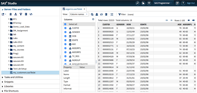
WARNING: When you load the data set into SAS you may get a warning message saying that it isn’t a SAS data set. What this means is that it is not a data set generated by SAS. But as you can see in the image above all the data got loaded OK and you can work away with it as normal in your SAS tools.
The next step is to test the loading of a SAS data set into R. I’m going to use one of the standard SAS data sets called PVA97NK.SAS7BDAT. If you have worked with SAS products then you will have come across this data set.
When you use Haven to load in your SAS data set, it will create the data in tribble format. This is a slight varient of a data.frame. So if you want the typical format of a data.frmae then you will need to convert the loaded data, as shown in the following code.
> data_read  dim(data_read)
[1] 9686   28
> d class(data_read)
[1] "tbl_df"     "tbl"        "data.frame"
> class(d)
[1] "data.frame"
> head(d)
  TARGET_B       ID TARGET_D GiftCnt36 GiftCntAll GiftCntCard36 GiftCntCardAll
1        0 00014974       NA         2          4             1              3
2        0 00006294       NA         1          8             0              3
3        1 00046110        4         6         41             3             20
...
I think this package to going to make my life a little bit easier, and if you work with SPSS and SAS data sets then hopefully some of your tasks have become a little bit easier too.
Machine Learning notebooks (and Oracle)
Over the past 12 months there has been an increase in the number of Machine Learning notebooks becoming available.
What is a Machine Learning notebook?
As the name implies it can be used to perform machine learning using one or more languages and allows you to organise your code, scripts and other details in one application.
The ML notebooks provide an interactive environment (sometimes browser based) that allows you to write, run, view results, share/collaborate code and results, visualise data, etc.
Some of these ML notebooks come with one language and others come with two or more languages, and have the ability to add other ML related languages. The most common languages are Spark, Phython and R.
Based on these languages ML notebooks are typically used in the big data world and on Hadoop.
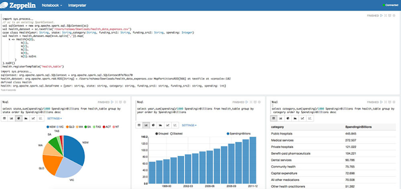
Examples of Machine Learning notebooks include: (Starting with the more common ones)
- Apache Zeppelin
- Jupyter Notebook (formally known as IPython Notebook)
- Azure ML R Notebook
- Beaker Notebook
- SageMath
At Oracle Open World (2016), Oracle announced that they are currently working creating their own ML notebook and it is based on Apache Zeppelin. They seemed to indicate that a beta version might be available in 2017. Here are some photos from that presentation, but with all things that Oracle talk about you have to remember and take into account their Safe Habor.
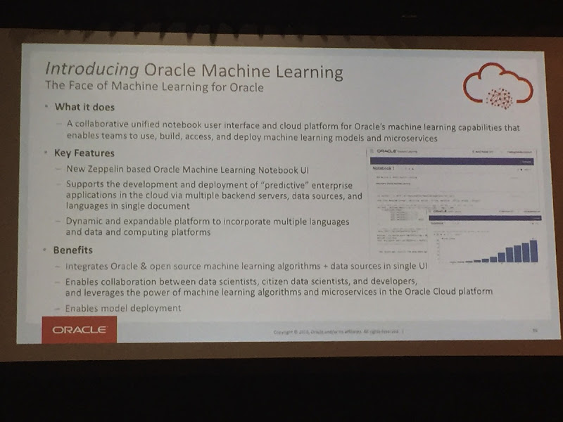
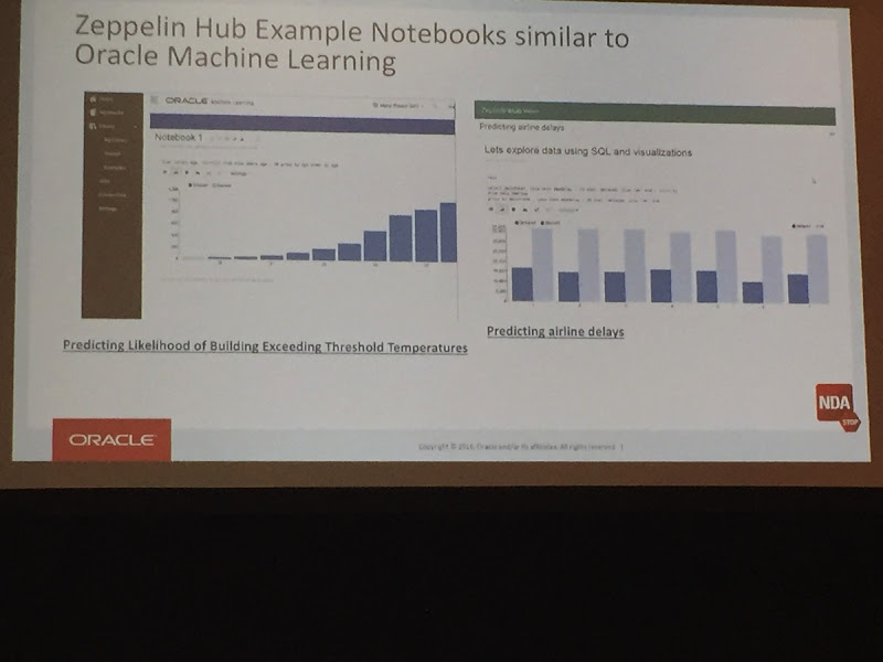
I’m looking forward to getting my hands on this new product when it is available.
Oracle Text, Oracle R Enterprise and Oracle Data Mining – Part 1
A project that I’ve been working on for a while now involves the use of Oracle Text, Oracle R Enterprise and Oracle Data Mining. Oracle Text comes with your Oracle Database licence. Oracle R Enterprise and Oracle Data Mining are part of the Oracle Advanced Analytics (extra cost) option.
What I will be doing over the course of 4 or maybe 5 blog posts is how these products can work together to help you gain a grater insight into your data, and part of your data being large text items like free format text, documents (in various forms e.g. html, xml, pdf, ms word), etc.
Unfortunately I cannot show you examples from the actual project I’ve been working on (and still am, from time to time). But what I can do is to show you how products and components can work together.
In this blog post I will just do some data setup. As with all project scenarios there can be many ways of performing the same tasks. Some might be better than others. But what I will be showing you is for demonstration purposes.
The scenario: The scenario for this blog post is that I want to extract text from some webpages and store them in a table in my schema. I then want to use Oracle Text to search the text from these webpages.
Schema setup: We need to create a table that will store the text from the webpages. We also want to create an Oracle Text index so that this text is searchable.
drop sequence my_doc_seq;
create sequence my_doc_seq;

drop table my_documents;

create table my_documents (
doc_pk number(10) primary key,
doc_title varchar2(100),
doc_extracted date,
data_source varchar2(200),
doc_text clob);

create index my_documents_ot_idx on my_documents(doc_text)
indextype is CTXSYS.CONTEXT;
In the table we have a number of descriptive attributes and then a club for storing the website text. We will only be storing the website text and not the html document (More on that later). In order to make the website text searchable in the DOC_TEXT attribute we need to create an Oracle Text index of type CONTEXT.
There are a few challenges with using this type of index. For example when you insert a new record or update the DOC_TEXT attribute, the new values/text will not be reflected instantly, just like we are use to with traditional indexes. Instead you have to decide when you want to index to be updated. For example, if you would like the index to be updated after each commit then you can create the index using the following.
create index my_documents_ot_idx on my_documents(doc_text)
indextype is CTXSYS.CONTEXT
parameters ('sync (on commit)');
Depending on the number of documents you have being committed to the DB, this might not be for you. You need to find the balance. Alternatively you could schedule the index to be updated by passing an interval to the ‘sync’ in the above command. Alternatively you might want to use DBMS_JOB to schedule the update.
To manually sync (or via DBMS_JOB) the index, assuming we used the first ‘create index’ statement, we would need to run the following.
EXEC CTX_DDL.SYNC_INDEX('my_documents_ot_idx');
This function just adds the new documents to the index. This can, over time, lead to some fragmentation of the index, and will require it to the re-organised on a semi-regular basis. Perhaps you can schedule this to happen every night, or once a week, or whatever makes sense to you.
BEGIN
  CTX_DDL.OPTIMIZE_INDEX('my_documents_ot_idx','FULL');
END;
(I could talk a lot more about setting up some basics of Oracle Text, the indexes, etc. But I’ll leave that for another day or you can read some of the many blog posts that already exist on the topic.)
Extracting text from a webpage using R: Some time ago I wrote a blog post on using some of the text mining features and packages in R to produce a word cloud based on some of the Oracle Advanced Analytics webpages.
I’m going to use the same webpages and some of the same code/functions/packages here.
The first task you need to do is to get your hands on the ‘htmlToText function. You can download the htmlToText function on github. This function requires the ‘Curl’ and ‘XML’ R packages. So you may need to install these.
I also use the str_replace_all function (“stringer’ R package) to remove some of the html that remains, to remove some special quotes and to replace and occurrences of ‘&’ with ‘and’.
# Load the function and required R packages
source(“c:/app/htmltotext.R”)
library(stringr)
data1 <- str_replace_all(htmlToText("http://www.oracle.com/technetwork/database/options/advanced-analytics/overview/index.html"), "[\r\n\t\"\'\u201C\u201D]" , "")
data1 <- str_replace_all(data1, "&", "and")
data2 <- str_replace_all(str_replace_all(htmlToText("http://www.oracle.com/technetwork/database/options/advanced-analytics/odm/index.html"), "[\r\n\t\"\'\u201C\u201D]" , ""), "&", "and")
data2 <- str_replace_all(data2, "&", "and")
data3 <- str_replace_all(str_replace_all(htmlToText("http://www.oracle.com/technetwork/database/database-technologies/r/r-technologies/overview/index.html"), "[\r\n\t\"\'\u201C\u201D]" , ""), "&", "and")
data3 <- str_replace_all(data3, "&", "and")
data4 <- str_replace_all(str_replace_all(htmlToText("http://www.oracle.com/technetwork/database/database-technologies/r/r-enterprise/overview/index.html"), "[\r\n\t\"\'\u201C\u201D]" , ""), "&", "and")
data4 <- str_replace_all(data4, "&", "and")
We now have the text extracted and cleaned up.
Create a data frame to contain all our data: Now that we have the text extracted, we can prepare the other data items we need to insert the data into our table (‘my_documents’). The first stept is to construct a data frame to contain all the data.
data_source = c("http://www.oracle.com/technetwork/database/options/advanced-analytics/overview/index.html",
                 "http://www.oracle.com/technetwork/database/options/advanced-analytics/odm/index.html",
                 "http://www.oracle.com/technetwork/database/database-technologies/r/r-technologies/overview/index.html",
                 "http://www.oracle.com/technetwork/database/database-technologies/r/r-enterprise/overview/index.html")
doc_title = c("OAA_OVERVIEW", "OAA_ODM", "R_TECHNOLOGIES", "OAA_ORE")
doc_extracted = Sys.Date()
data_text <- c(data1, data2, data3, data4)

my_docs <- data.frame(doc_title, doc_extracted, data_source, data_text)
Insert the data into our database table: With the data in our data fram (my_docs) we can now use this data to insert into our database table. There are a number of ways of doing this in R. What I’m going to show you here is how to do it using Oracle R Enterprise (ORE). The thing with ORE is that there is no explicit functionality for inserting and updating records in a database table. What you need to do is to construct, in my case, the insert statement and then use ore.exec to execute this statement in the database.
googleVis R package for creating google charts in R
I’ve recently come across the ‘googleVis’ R package. This allows you to create a variety of different (typical and standard) charts in R but with the look and feel of the charts we can get from a number of different Google sites.
I won’t bore you with some examples in the post but I’ll point you to a good tutorial on the various charts.
Here is the link to the mini-tutorial.
Before you can use the package you will need to install it. The simplest way is to run the following in your R session.
> install.packages("googleVis")
Depending on your version of R you may need to upgrade.
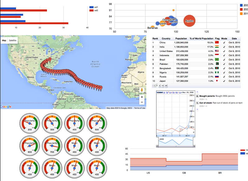
Here is a selection of some of the charts you can create, and there are many, many more.
Some of you might be familiar with the presenting that Hans Rosling gives. Some of the same technology is behind these bubble charts from Google, as they bought the software years ago. Hans typically uses a data set that consists of GDP, Population and Life Expectancy for countries around the World. You too can use this same data set and is available from rdatamarket. The following R codes will extract this data set to you local R session and you can then use it as input to the various charts in the googleVis functions.
install.packages("rdatamarket")
library(rdatamarket)
dminit(NULL)

# Pull in life expectancy and population data
life_expectancy <- dmlist("15r2!hrp")
population <- dmlist("1cfl!r3d")

# Pull in the yearly GDP for each country
gdp <- dmlist("15c9!hd1")

# Load in the plyr package
library("plyr")

# Rename the Value for each dataset
names(gdp)[3] <- "GDP"

# Use plyr to join your three data frames into one: development
gdp_life_exp <- join(gdp, life_expectancy)
names(gdp_life_exp)[4] <- "LifeExpectancy"
development <- join(gdp_life_exp, population)
names(development)[5] <- "Population"
Here is an example of the bubble chart using this data set.
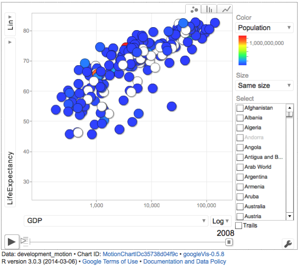
There are a few restrictions with using this package. All the results will be displayed in a web browser, so you need to make sure that this is possible. Some of the charts are require flash. Again you need to make sure you are the latest version and/or you many have restrictions in your workplace on using it.
Accessing the R datasets in ORE and SQL
When you install R you also get a set of pre-compiled datasets. These are great for trying out many of the features that are available with R and all the new packages that are being produced on an almost daily basis.
The exact list of data sets available will depend on the version of R that you are using.
To get the list of available data sets in R you can run the following.
> library(help="datasets")
This command will list all the data sets that you can reference and start using immediately.
I’m currently running the latest version of Oracle R Distribution version 3.2. See the listing at the end of this blog post for the available data sets.
But are these data sets available to you if you are using Oracle R Enterprise (ORE)? The answer is Yes of course they are.
But are these accessible on the Oracle Database server? Yes they are, as you have R installed there and you can use ORE to access and use the data sets.
But how? how can I list what is on the Oracle Database server using R? Simple use the following ORE code to run an embedded R execution function using the ORE R API.
What? What does that mean? Using the R on your client machine, you can use ORE to send some R code to the Oracle Database server. The R code will be run on the Oracle Database server and the results will be returned to the client. The results contain the results from the server. Try the following code.
ore.doEval(function() library(help="datasets"))

# let us create a functions for this code
myFn <- function() {library(help="datasets")}

# Now send this function to the DB server and run it there.
ore.doEval(myFn)

# create an R script in the Oracle Database that contains our R code
ore.scriptDrop("inDB_R_DemoData")
ore.scriptCreate("inDB_R_DemoData", myFn)
# Now run the R script, stored in the Oracle Database, on the Database server
#   and return the results to my client
ore.doEval(FUN.NAME="inDB_R_DemoData")
Simple, Right!
Yes it is. You have shown us how to do this in R using the ORE package. But what if I’m a SQL developer. Can I do this in SQL? Yes you can. Connect you your schema using SQL Developer/SQL*Plus/SQLcl or whatever tool you will be using to run SQL. Then run the following SQL.
select *
from table(rqEval(null, 'XML', 'inDB_R_DemoData'));
This SQL code will return the results in XML format. You can parse this to extract and display the results and when you do you will get something like the following listing, which is exactly the same that is produced when you run the R code that I gave above.
So what this means is that evening if you have an empty schema with no data in it, and as long as you have the privileges to run embedded R execution, you actually have access to all these different data sets. You can use these to try our R using the ORE SQL APIs too.
		Information on package ‘datasets’

Description:

Package:       datasets
Version:       3.2.0
Priority:      base
Title:         The R Datasets Package
Author:        R Core Team and contributors worldwide
Maintainer:    R Core Team
Description:   Base R datasets.
License:       Part of R 3.2.0
Built:         R 3.2.0; ; 2015-08-07 02:20:26 UTC; windows

Index:

AirPassengers           Monthly Airline Passenger Numbers 1949-1960
BJsales                 Sales Data with Leading Indicator
BOD                     Biochemical Oxygen Demand
CO2                     Carbon Dioxide Uptake in Grass Plants
ChickWeight             Weight versus age of chicks on different diets
DNase                   Elisa assay of DNase
EuStockMarkets          Daily Closing Prices of Major European Stock
                        Indices, 1991-1998
Formaldehyde            Determination of Formaldehyde
HairEyeColor            Hair and Eye Color of Statistics Students
Harman23.cor            Harman Example 2.3
Harman74.cor            Harman Example 7.4
Indometh                Pharmacokinetics of Indomethacin
InsectSprays            Effectiveness of Insect Sprays
JohnsonJohnson          Quarterly Earnings per Johnson & Johnson Share
LakeHuron               Level of Lake Huron 1875-1972
LifeCycleSavings        Intercountry Life-Cycle Savings Data
Loblolly                Growth of Loblolly pine trees
Nile                    Flow of the River Nile
Orange                  Growth of Orange Trees
OrchardSprays           Potency of Orchard Sprays
PlantGrowth             Results from an Experiment on Plant Growth
Puromycin               Reaction Velocity of an Enzymatic Reaction
Theoph                  Pharmacokinetics of Theophylline
Titanic                 Survival of passengers on the Titanic
ToothGrowth             The Effect of Vitamin C on Tooth Growth in
                        Guinea Pigs
UCBAdmissions           Student Admissions at UC Berkeley
UKDriverDeaths          Road Casualties in Great Britain 1969-84
UKLungDeaths            Monthly Deaths from Lung Diseases in the UK
UKgas                   UK Quarterly Gas Consumption
USAccDeaths             Accidental Deaths in the US 1973-1978
USArrests               Violent Crime Rates by US State
USJudgeRatings          Lawyers' Ratings of State Judges in the US
                        Superior Court
USPersonalExpenditure   Personal Expenditure Data
VADeaths                Death Rates in Virginia (1940)
WWWusage                Internet Usage per Minute
WorldPhones             The World's Telephones
ability.cov             Ability and Intelligence Tests
airmiles                Passenger Miles on Commercial US Airlines,
                        1937-1960
airquality              New York Air Quality Measurements
anscombe                Anscombe's Quartet of 'Identical' Simple Linear
                        Regressions
attenu                  The Joyner-Boore Attenuation Data
attitude                The Chatterjee-Price Attitude Data
austres                 Quarterly Time Series of the Number of
                        Australian Residents
beavers                 Body Temperature Series of Two Beavers
cars                    Speed and Stopping Distances of Cars
chickwts                Chicken Weights by Feed Type
co2                     Mauna Loa Atmospheric CO2 Concentration
crimtab                 Student's 3000 Criminals Data
datasets-package        The R Datasets Package
discoveries             Yearly Numbers of Important Discoveries
esoph                   Smoking, Alcohol and (O)esophageal Cancer
euro                    Conversion Rates of Euro Currencies
eurodist                Distances Between European Cities and Between
                        US Cities
faithful                Old Faithful Geyser Data
freeny                  Freeny's Revenue Data
infert                  Infertility after Spontaneous and Induced
                        Abortion
iris                    Edgar Anderson's Iris Data
islands                 Areas of the World's Major Landmasses
lh                      Luteinizing Hormone in Blood Samples
longley                 Longley's Economic Regression Data
lynx                    Annual Canadian Lynx trappings 1821-1934
morley                  Michelson Speed of Light Data
mtcars                  Motor Trend Car Road Tests
nhtemp                  Average Yearly Temperatures in New Haven
nottem                  Average Monthly Temperatures at Nottingham,
                        1920-1939
npk                     Classical N, P, K Factorial Experiment
occupationalStatus      Occupational Status of Fathers and their Sons
precip                  Annual Precipitation in US Cities
presidents              Quarterly Approval Ratings of US Presidents
pressure                Vapor Pressure of Mercury as a Function of
                        Temperature
quakes                  Locations of Earthquakes off Fiji
randu                   Random Numbers from Congruential Generator
                        RANDU
rivers                  Lengths of Major North American Rivers
rock                    Measurements on Petroleum Rock Samples
sleep                   Student's Sleep Data
stackloss               Brownlee's Stack Loss Plant Data
state                   US State Facts and Figures
sunspot.month           Monthly Sunspot Data, from 1749 to "Present"
sunspot.year            Yearly Sunspot Data, 1700-1988
sunspots                Monthly Sunspot Numbers, 1749-1983
swiss                   Swiss Fertility and Socioeconomic Indicators
                        (1888) Data
treering                Yearly Treering Data, -6000-1979
trees                   Girth, Height and Volume for Black Cherry Trees
uspop                   Populations Recorded by the US Census
volcano                 Topographic Information on Auckland's Maunga
                        Whau Volcano
warpbreaks              The Number of Breaks in Yarn during Weaving
women                   Average Heights and Weights for American Women
Configuring RStudio Server for Oracle R Enterprise
In this blog post I will show you the configurations that are necessary for RStudio Server to work with Oracle R Enterprise on your Oracle Database server. In theory if you have just installed ORE and then RStudio Server, everything should work, but if you encounter any issues then check out the following.
Before I get started make sure to check out my previous blog posts on installing R Studio Server. The first blog post was installing and configuring RStudio Server on the Oracle BigDataLite VM. This is an automated install. The second blog post was a step by step guide to installing RStudio Server on your (Oracle) Linux Database Server and how to open the port on the VM using VirtualBox.
Right. Let’s get back to configuring to work with Oracle R Enterprise. The following assumes you have complete the second blog post mentioned above.
1. Edit the rserver.conf files
Add in the values and locations for RHOME and ORACLE_HOME
sudo vi /etc/rstudio/rserver.conf
    rsession-ld-library-path=RHOME/lib:ORACLE_HOME/lib
2. Edit the .Renviron file.
Add in the values for ORACLE_HOME, ORACLE_HOSTNAME and ORACLE_SID
cd /home/oracle
sudo vi .Renviron
    ORACLE_HOME=ORACLE_HOME
    ORACLE_HOSTNAME=ORACLE_HOSTNAME
    ORACLE_SID=ORACLE_SID

export ORACLE_HOME
export ORACLE_HOSTNAME
export ORACLE_SID
3. To access the Oracle R Distribution
Add the following to the usr/lib/rstudio-server/R/modules/SessionHelp.R file for the version of Oracle R Distribution you installed prior to installing Oracle R Enterprise.
.rs.addFunction( "httpdPortIsFunction", function() {
   getRversion() >= "3.2"
})
You are all done now with all the installations and configurations.


You must be logged in to post a comment.