
statistics
Measuring Kurtosis of Data in Oracle (21c)
Kurtosis is a new analytics function in Oracle 21c (20c) and is one of a set of commonly used statistical functions used to evaluate data to see and understand the behavior of the data.
[See my previous post where I give examples of the new Skewness functions]
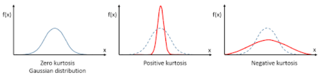
Kurtosis is the measurement of the tails of the data distribution and its comparison with that of normal distribution. The Kurtosis of the normal distribution is said to be 3. To make interpenetrating results easier (a Zero) kurtosis measure for gaussian/normal distribution by subtracting 3 from its value, this is called Excess Kurtosis. Kurtosis can be used to describe the height or the breath of the distributions, when compared to a normal distributions, although this is not theoretically correct, it gives a simpler explanation and visualization of it. The following diagram gives an example of a normal distribution, a plot of Positive Kurtosis and Negative Kurtosis.
Prior to the new Kurtosis SQL functions (KURTOSIS_POP and KURTOSIS_SAMP), you had to calculate the Kurtosis value manually using something like the following SQL. These use the same data and attributes set used for the Skewness examples.
select avg(KV) K_value
from (select power((age - avg(age) over ())/stddev(age) over (), 4) KV
      from cust_data)
union all
select avg(KV) K_value
from (select power((duration - avg(duration) over ())/stddev(duration) over (), 4) KV
      from cust_data);

K_value
------------------------------------------
3.79088571963003808388287765230733611415
23.24420570926391173498028369605428048285
These don’t include the subtraction of 3 to give a zero kurtosis, and these values can be compared to the data distribution charts shown in the Skewness post.
Now with the new Kurtosis functions it simplifies the tasks of getting these values.
SELECT kurtosis_pop(age), kurtosis_samp(age)
FROM bank_additional
union all
SELECT kurtosis_pop(duration), kurtosis_samp(duration)
FROM bank_additional;

KURTOSIS_POP         KURTOSIS_SAMP
------------------   -----------------------------------------
 0.791069803527387    0.79131153115443467194451597661213420763
20.245334438614832   20.24793801497878942299945619307526969226
As you can see the Kurtosis function have the subtraction include.
As with the Skewness functions, the SAMP version works on a sample of the data values and as the number inputs increases, and differences between the POP and SAMP will reduce.
Measuring Skewness of Data in Oracle (21c)
When analyzing data you will look at using a variety of different statistical functions to explore variable data insights.
One of these is the Skewness of the data.
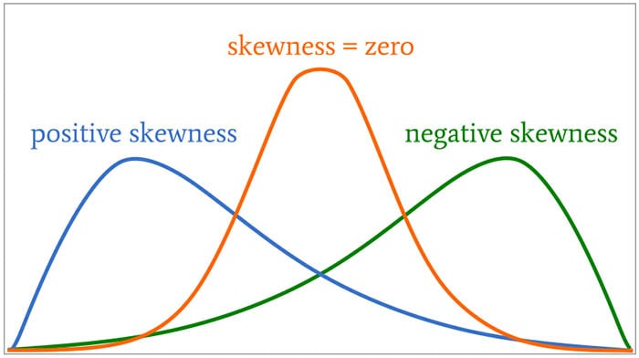
Skewness is a measure of the asymmetry of the probability distribution about its mean. This looks a the tail of the data, with a positive value indicating the tail on the right side of the distribution, and a negative value when the tail is on the left hand side. A zero value indicates the tails on both side balance out, as shown in the following image.
Most SQL dialects support Skewness using with an inbuilt function. But if it doesn’t then you would need to write your own version of the calculation, for example using the following.
SELECT avg(SV) S_value
FROM   (SELECT  power((age – avg(age) over ())/stddev(age) over (), 3) SV
        FROM    cust_data)
Here are charts illustrating the data in my table. These include the distributions for the AGE and DURATION attributes.
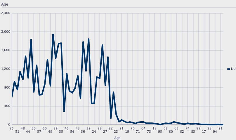

We can see the data is skewed. When we run the above code we get the following values.
Age = 0.78
Duration = 3.26
We can see the skewness of Duration is significantly longer, giving a positive value as the skewness is to the right.
In Oracle 21s we now have new Skewness functions called SKEWNESS_POP and SKEWNESS_SAMP. The POP version of the function considers all records, where as the SAMP function considers a sample of the records. When your data set grows into many millions of records the SKEWNESS_SAMP will give a quicker response as it works with a sample of the data set
Both functions will give similar values but at the number of input records the returned values will returned will converge.
SELECT skewness_pop(age), skewness_samp(age)
FROM cust_data;
SELECT skewness_pop(duration), skewness_samp(duration)
FROM cust_data;

Managing imbalanced Data Sets with SMOTE in Python
When working with data sets for machine learning, lots of these data sets and examples we see have approximately the same number of case records for each of the possible predicted values. In this kind of scenario we are trying to perform some kind of classification, where the machine learning model looks to build a model based on the input data set against a target variable. It is this target variable that contains the value to be predicted. In most cases this target variable (or feature) will contain binary values or equivalent in categorical form such as Yes and No, or A and B, etc or may contain a small number of other possible values (e.g. A, B, C, D).
For the classification algorithm to perform optimally and be able to predict the possible value for a new case record, it will need to see enough case records for each of the possible values. What this means, it would be good to have approximately the same number of records for each value (there are many ways to overcome this and these are outside the score of this post). But most data sets, and those that you will encounter in real life work scenarios, are never balanced, as in having a 50-50 split. What we typically encounter might be a 90-10, 98-2, etc type of split. These data sets are said to be imbalanced.

The image above gives examples of two approaches for creating a balanced data set. The first is under-sampling. This involves reducing the class that contains the majority of the case records and reducing it to match the number of case records in the minor class. The problems with this include, the resulting data set is too small to be meaningful, the case records removed could contain important records and scenarios that the model will need to know about.
The second example is creating a balanced data set by increasing the number of records in the minority class. There are a few approaches to creating this. The first approach is to create duplicate records, from the minor class, until such time as the number of case records are approximately the same for each class. This is the simplest approach. The second approach is to create synthetic records that are statistically equivalent of the original data set. A commonly technique used for this is called SMOTE, Synthetic Minority Oversampling Technique. SMOTE uses a nearest neighbors algorithm to generate new and synthetic data we can use for training our model. But one of the issues with SMOTE is that it will not create sample records outside the bounds of the original data set. As you can image this would be very difficult to do.
The following examples will illustrate how to perform Under-Sampling and Over-Sampling (duplication and using SMOTE) in Python using functions from Pandas, Imbalanced-Learn and Sci-Kit Learn libraries.
NOTE: The Imbalanced-Learn library (e.g. SMOTE)requires the data to be in numeric format, as it statistical calculations are performed on these. The python function get_dummies was used as a quick and simple to generate the numeric values. Although this is perhaps not the best method to use in a real project. With the other sampling functions can process data sets with a sting and numeric.
Data Set: Is the Portuaguese Banking data set and is available on the UCI Data Set Repository, and many other sites. Here are some basics with that data set.
import warnings

import pandas as pd
import numpy as np
import matplotlib.pyplot as plt
get_ipython().magic('matplotlib inline')

bank_file = ".../bank-additional-full.csv"

# import dataset
df = pd.read_csv(bank_file, sep=';',)

# get basic details of df (num records, num features)
df.shape
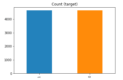
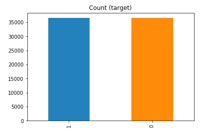
df['y'].value_counts() # dataset is imbalanced with majority of class label as "no".
no     36548
yes     4640
Name: y, dtype: int64
#print bar chart
df.y.value_counts().plot(kind='bar', title='Count (target)');

Example 1a – Down/Under sampling the majority class y=1 (using random sampling)
count_class_0, count_class_1 = df.y.value_counts()

# Divide by class
df_class_0 = df[df['y'] == 0] #majority class
df_class_1 = df[df['y'] == 1] #minority class

# Sample Majority class (y=0, to have same number of records as minority calls (y=1)
df_class_0_under = df_class_0.sample(count_class_1)
# join the dataframes containing y=1 and y=0
df_test_under = pd.concat([df_class_0_under, df_class_1])

print('Random under-sampling:')
print(df_test_under.y.value_counts())
print("Num records = ", df_test_under.shape[0])

df_test_under.y.value_counts().plot(kind='bar', title='Count (target)');
Example 1b – Down/Under sampling the majority class y=1 using imblearn
from imblearn.under_sampling import RandomUnderSampler

X = df_new.drop('y', axis=1)
Y = df_new['y']

rus = RandomUnderSampler(random_state=42, replacement=True)
X_rus, Y_rus = rus.fit_resample(X, Y)

df_rus = pd.concat([pd.DataFrame(X_rus), pd.DataFrame(Y_rus, columns=['y'])], axis=1)

print('imblearn over-sampling:')
print(df_rus.y.value_counts())
print("Num records = ", df_rus.shape[0])

df_rus.y.value_counts().plot(kind='bar', title='Count (target)');
[same results as Example 1a]
Example 1c – Down/Under sampling the majority class y=1 using Sci-Kit Learn
from sklearn.utils import resample

print("Original Data distribution")
print(df['y'].value_counts())

# Down Sample Majority class
down_sample = resample(df[df['y']==0],
replace = True, # sample with replacement
n_samples = df[df['y']==1].shape[0], # to match minority class
random_state=42) # reproducible results

# Combine majority class with upsampled minority class
train_downsample = pd.concat([df[df['y']==1], down_sample])

# Display new class counts
print('Sci-Kit Learn : resample : Down Sampled data set')
print(train_downsample['y'].value_counts())
print("Num records = ", train_downsample.shape[0])
train_downsample.y.value_counts().plot(kind='bar', title='Count (target)');
[same results as Example 1a]
Example 2 a – Over sampling the minority call y=0 (using random sampling)
df_class_1_over = df_class_1.sample(count_class_0, replace=True)
df_test_over = pd.concat([df_class_0, df_class_1_over], axis=0)

print('Random over-sampling:')
print(df_test_over.y.value_counts())

df_test_over.y.value_counts().plot(kind='bar', title='Count (target)');
Random over-sampling:
1    36548
0    36548
Name: y, dtype: int64
Example 2b – Over sampling the minority call y=0 using SMOTE
from imblearn.over_sampling import SMOTE

print(df_new.y.value_counts())
X = df_new.drop('y', axis=1)
Y = df_new['y']

sm = SMOTE(random_state=42)
X_res, Y_res = sm.fit_resample(X, Y)

df_smote_over = pd.concat([pd.DataFrame(X_res), pd.DataFrame(Y_res, columns=['y'])], axis=1)

print('SMOTE over-sampling:')
print(df_smote_over.y.value_counts())

df_smote_over.y.value_counts().plot(kind='bar', title='Count (target)');
[same results as Example 2a]
Example 2c – Over sampling the minority call y=0 using Sci-Kit Learn
from sklearn.utils import resample

print("Original Data distribution")
print(df['y'].value_counts())

# Upsample minority class
train_positive_upsample = resample(df[df['y']==1],
replace = True, # sample with replacement
n_samples = train_zero.shape[0], # to match majority class
random_state=42) # reproducible results

# Combine majority class with upsampled minority class
train_upsample = pd.concat([train_negative, train_positive_upsample])

# Display new class counts
print('Sci-Kit Learn : resample : Up Sampled data set')
print(train_upsample['y'].value_counts())
train_upsample.y.value_counts().plot(kind='bar', title='Count (target)');
[same results as Example 2a]
Oracle Code Online December 2017
This week Oracle Code will be having an online event consisting of 5 tracks and with 3 presentations on each track.
This online Oracle Code event will be given in 3 different geographic regions on 12th, 13th and 14th December.

I’ve been selected to give one of these talks, and I’ve given this talk at some live Oracle Code events and at JavaOne back in October.
The present is pre-recorded and I recorded this video back in September.
I hope to be online at the end of some of these presentations to answer any questions, but unfortunately due to changes with my work commitments I may not be able to be online for all of them.
The moderator for these events will take your questions (or you can send them to me here) and I will write a blog post answering all your questions.

You must be logged in to post a comment.