Oracle Advanced Analytics
New OAA features in Oracle 12.2 Database
The Oracle 12.2c Database has been released and is currently available as a Cloud Service. The on-site version should be with us soon.
A few weeks ago I listed some of the new features that you will find in the Oracle Data Miner GUI tool (check out that blog post). I’ll have another blog post soon that looks a bit closer at how the new OAA features are exposed in this tool.
In this blog post I will list most of the new database related features in Oracle 12.2. There is a lot of new features and a lot of updated features. Over the next few months (yes it will take that long) I’ll have blog posts on most of these.
The Oracle Advanced Analytics Option new features include:
- The first new feature is one that you cannot see. Yes that sound a bit odd. But the underlying architecture of OAA has been rebuilt to allow for the algorithms to scale significantly. This is also future proofing OAA for new features coming in future releases of the database.
- Explicit Semantic Analysis. This is a new algorithm allows us to perform text similarity comparison. This is a great new addition and and much, much easier now compared to what we may have had to do previously.
- Using R models using SQL. Although we have been able to do this in the previous version of the database, the framework and supports have been extended to allow for greater and easier usage of user defined R scripts and R models with the in-database environment.
- Partitioned Models. We can now build partitioned mining models. This is where you can specify an attribute and a separate model will be created based on each value in the attribute.
- Partitioned scoring. Similarly we can now dynamically score the data based on an partition attribute.
- Extentions to Association Rules. Over the past few releases of the database, additional insights to the workings and decision making of the algorithms have been included. In 12.2 we now have some additional insights for the Association Rules aglorithm where we can now get to see the calculation of values associated with rules.
- DBMS_DATA_MINING package extended. This PL/SQL package has been extended to include the functionality for the new features listed above. Additional it can now process R algorithms and models.
- SQL Function changes: Change to the followi ODM related SQL functions to allow for partitioned models. CLUSTER_DETAILS, CLUSTER_DISTANCE, CLUSTER_ID, CLUSTER_PROBABILITY, CLUSTER_SET, FEATURE_COMPARE, FEATURE_DETAILS, FEATURE_ID, FEATURE_SET, FEATURE_VALUE, ORA_DM_PARTITION_NAME, PREDICTION, PREDICTION_BOUNDS, PREDICTION_COST, PREDICTION_DETAILS, PREDICTION_PROBABILITY, PREDICTION_SET
- New SQL Hint for ODM models. We have had hints in SQL for many, many versions now, but with 12.2c we now have a hint for partitioned models, called GROUPING hint.
- New CREATE_MODEL function. With the existing CREATE_MODEL function the input data set for the function needed to be defined in a table or accessed using a view. Basically the data needed to resist somewhere. With CREAETE_MODEL2 you can now define the input data set based on a SELECT statement.
In addition to all of these changes there are also some new interesting DB, SQL and PL/SQL new features that are of particular interest for your data science, machine learning, advanced analytics (or whatever the current favourite marketing term is today) projects.
It is going to be a busy few months ahead, working through all of these new features and write blog posts on how to use each of them.
Oracle Text, Oracle R Enterprise and Oracle Data Mining – Part 5
In this 5th blog post in my series on using the capabilities of Oracle Text, Oracle R Enterprise and Oracle Data Mining to process documents and text, I will have a look at some of the machine learning features of Oracle Text.
Oracle Text comes with a number of machine learning algorithms. These can be divided into two types. The first is called ‘Supervised Learning’ where we have two machine learning algorithms for classification type of problem. The second type is called ‘Unsupervised Learning’ where we have the ability to use clustering machine learning algorithms to look for patterns in our text documents and to find similarities between documents based on their contents.
It is this second type of document clustering that I will work through in this blog post.
When using clustering with text documents, the machine learning algorithm will look for patterns that are common between the documents. These patterns will include the words used, the frequency of the words, the position or ordering of these words, the co-occurance of words, etc. Yes this is a large an complex task and that is why we need a machine learning algorithm to help us.
With Oracle Text we only have one clustering machine learning algorithm available to use. When we move onto using the Oracle Advanced Analytics Option (Oracle Data Mining and Oracle R Enterprise) we more algorithms available to us.
With Oracle Text the clustering algorithm is called k-Means. In a way the actual algorithm is unimportant as it is the only one available to us when using Oracle Text. To use this algorithm we have the CTX_CLS.CLUSTERING procedure. This procedure takes the documents we want to compare and will then identify the clusters (using hierarchical clustering) and will then tells us, for each document, what clusters the documents belong to and they probability value. With clustering a document (or a record) can belong to many clusters. Typically in the text books we see clusters that are very distinct and are clearly separated from each other. When you work on real data this is never the case. We will have many over lapping clusters and a data point/record can belong to one or more clusters. This is why we need the probability vale. We can use this to determine what cluster our record belongs to most and what other clusters it is associated with.
Using the example documents that I have been using during this series of blog posts we can use the CTX_CLS.CLUSTERING algorithm to cluster and identify similarities in these documents.
We need to setup the parameters that will be used by the CTX_CLS.CLUSTERING procedure. Tell it to use the k-Means algorithm and then the number of clusters to generate. As with all Oracle Text procedures or algorithms there are a number of settings you can configure or you can just accept the default values.
exec ctx_ddl.drop_preference('Cluster_My_Documents');
exec ctx_ddl.create_preference('Cluster_My_Documents','KMEAN_CLUSTERING');
exec ctx_ddl.set_attribute('Cluster_My_Documents','CLUSTER_NUM','3');
The code above is an example of the basics of what you need to setup for clustering. Other attribute or cluster parameter setting available to you include, MAX_DOCTERMS, MAX_FEATURES, THEME_ON, TOKEN_ON, STEM_ON, MEMORY_SIZE and SECTION_WEIGHT.
Now we can run the CTX_CLS.CLUSTERING procedure on our documents. This procedure has the following parameters.
– The Oracle Text Index Name
– Document Id Column Name
– Document Assignment (cluster assignment) Table Name. This table will be created if it doesn’t already exist
– Cluster Description Table Name. This table will be created if it doesn’t already exist.
– Name of the Oracle Text Preference (list)
exec ctx_cls.clustering(
'MY_DOCUMENTS_OT_IDX',
'DOC_PK',
'OT_CLUSTER_RESULTS',
'DOC_CLUSTER_DETAILS',
'Cluster_My_Documents');
When the procedure has completed we can now examine the OT_CLUSTER_RESULTS and the DOC_CLUSTER_DETAILS tables. The first of these (OT_CLUSTER_RESULTS) allows us to see what documents have been clustered together. The following is what was produced for my documents.
SELECT d.doc_pk,
       d.doc_title,
       r.clusterid,
       r.score
FROM my_documents d,
     ot_cluster_results r
WHERE d.doc_pk = r.docid;
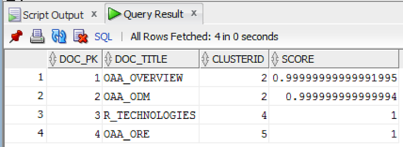
We can see that two of the documents have been grouped into the same cluster (ClusterId=2). If you have a look back at what these documents are about then you can see that yes these are very similar. For the other two documents we can see that they have been clustered into separate clusters (ClusterId=4 & 5). The clustering algorithms have said that they are different types of documents. Again when you examine these documents you will see that they are talking about different topics. So the clustering process worked !
You can also explore the various features of the clusters by looking that he DOC_CLUSTER_DETAILS table. Although the details in this table are not overly useful but it will give you some insight into what clusters the k-Means algorithm has produced.
Hopefully I’ve shown you how easy it is to setup and use the clustering feature of Oracle Text.
WARNING: Before using the Clustering or Classification with Oracle Text, you need to check with your local Oracle Sales representative about if there is licence implication. There seems to be some mentions the the algorithms used are those that come with Oracle Data Mining. Oracle Data Mining is a licence cost option for the database. So make sure you check before you go using these features.
How to get ORE to work with APEX
This blog post will bring you through the steps of how to get Oracle R Enterprise (ORE) to work with APEX.
The reason for this blog posts is that since ORE 1.4+ the security model has changed for how you access and run in-database user defined R scripts using the ORE SQL API functions.
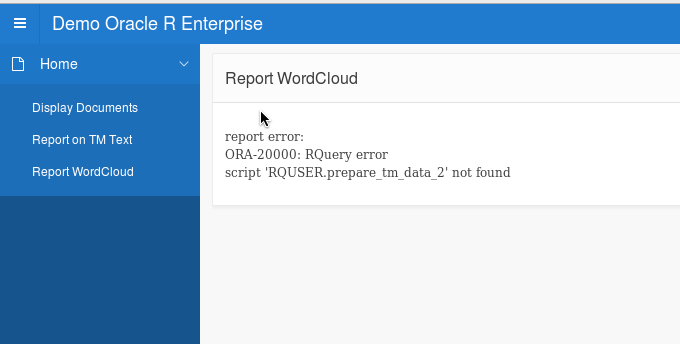
I have a series of blog posts going out on using Oracle Text, Oracle R Enterprise and Oracle Data Mining. It was during one of these posts I wanted to show how easy it was to display an R chart using ORE in APEX. Up to now my APEX environment consisted of APEX 4 and ORE 1.3. Everything worked, nice and easy. But in my new APEX environment (APEX 5 and ORE 1.5), it didn’t work. This is the calling of an in-database user defined R script using the SQL API functions didn’t work. Here is the error message that is displayed.
So something extra was needed with using ORE 1.5. The security model around the use of in-database user defined R scripts has changed. Extra functions are now available to allow you who can run these scripts. For example we have an ore.grant function where you can grant another user the privilege to run the script.
But the problem was, when I was in APEX, the application was defined on the same schema that the r script was created in (this was the RQUSER schema). When I connect to the RQUSER schema using ORE and SQL, I was able to see and run this R script (see my previous blog post for these details). But when I was in APEX I wasn’t able to see the R script. For example, when using the SQL Workshop in APEX, I just couldn’t see the R script.
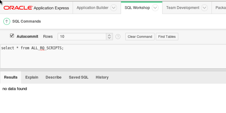
Something strange is going on. It turns out that the view definitions for the in-database ORE scripts are defined with
owner=SYS_CONTEXT('USERENV', 'SESSION_USER');
(Thanks to the Oracle ORE team and the Oracle APEX team for their help in working out what needed to be done)
This means when I’m connected to APEX, using my schema (RQUSER), I’m not able to see any of my ORE objects.
How do you overcome this problem ?
To fix this problem, I needed to grant the APEX_PUBLIC_USER access to my ORE script.
ore.grant(name = "prepare_tm_data_2", type = "rqscript", user = "APEX_PUBLIC_USER")
Now when I query the ALL_RQ_SCRIPTS view again, using the APEX SQL Workshop, I now get the following.
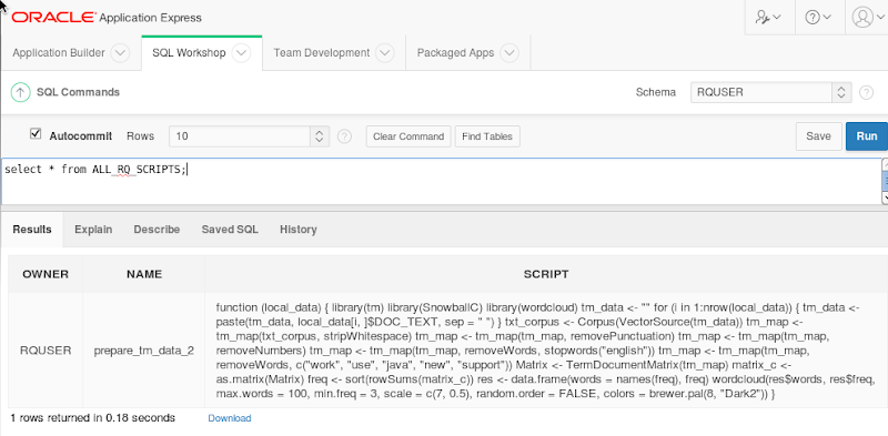
Great. Now I can see the ORE script in my schema.
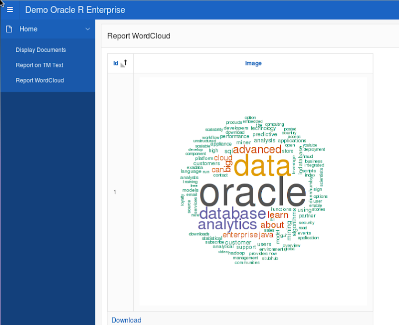
Now when I run my APEX application I now get graphic produced by R, running on my DB server, and delivered to my APEX application using SQL (via a BLOB object), displayed on my screen.
Change the size of ORE PNG graphics using in-database R functions
In a previous blog post I showed you how create and display a ggplot2 R graphic using SQL. Make sure to check it out before reading the rest of this blog post.
In my previous blog post, I showed and mentioned that the PNG graphic returned by the embedded R execution SQL statement was not the same as what was produced if you created the graphic in an R session.
Here is the same ggplot2 graphic. The first one is what is produced in an R session and the section is what is produced by SQL query and the embedded R execution in Oracle.

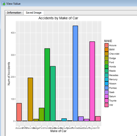
As you can see the second image (produced using the embedded R execution) gives a very square image.
The reason for this is that Oracle R Enterprise (ORE) creates the graphic image in PNG format. The default setting from this is 480 x 480. You will find this information when you go digging in the R documentation and not in the Oracle documentation.
So, how can I get my ORE produced graphic to appear like what is produced in R?
What you need to do is to change the height and width of the PNG image produced by ORE. You can do this by passing parameters in the SQL statement used to call the user defined R function, that in turn produces the ggplot2 image.
In my previous post, I gave the SQL statement to call and produce the graphic (shown above). One of the parameters to the rqTableEval function was set to null. This was because we didn’t have any parameters to pass, apart from the data set.
We can replace this null with any parameters we want to pass to the user defined R function (demo_ggpplot). To pass the parameters we need to define them using a SELECT statement.
cursor(select 500 as "ore.png.height", 850 as "ore.png.width" from dual),
The full SELECT statement now becomes
select *
from table(rqTableEval( cursor(select * from claims),
                        cursor(select 500 as "ore.png.height", 850 as "ore.png.width" from dual),
                        'PNG',
                        'demo_ggpplot'));
When you view the graphic in SQL Developer, you will get something that looks a bit more like what you would expect or want to see.
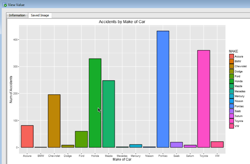
For each graphic image you want to produce using ORE you will need to figure out that are the best PNG height and width settings to use. Plus it also depends on what tool or application you are going to use to display the images (eg. APEX etc)
Oracle Text, Oracle R Enterprise and Oracle Data Mining – Part 1
A project that I’ve been working on for a while now involves the use of Oracle Text, Oracle R Enterprise and Oracle Data Mining. Oracle Text comes with your Oracle Database licence. Oracle R Enterprise and Oracle Data Mining are part of the Oracle Advanced Analytics (extra cost) option.
What I will be doing over the course of 4 or maybe 5 blog posts is how these products can work together to help you gain a grater insight into your data, and part of your data being large text items like free format text, documents (in various forms e.g. html, xml, pdf, ms word), etc.
Unfortunately I cannot show you examples from the actual project I’ve been working on (and still am, from time to time). But what I can do is to show you how products and components can work together.
In this blog post I will just do some data setup. As with all project scenarios there can be many ways of performing the same tasks. Some might be better than others. But what I will be showing you is for demonstration purposes.
The scenario: The scenario for this blog post is that I want to extract text from some webpages and store them in a table in my schema. I then want to use Oracle Text to search the text from these webpages.
Schema setup: We need to create a table that will store the text from the webpages. We also want to create an Oracle Text index so that this text is searchable.
drop sequence my_doc_seq;
create sequence my_doc_seq;

drop table my_documents;

create table my_documents (
doc_pk number(10) primary key,
doc_title varchar2(100),
doc_extracted date,
data_source varchar2(200),
doc_text clob);

create index my_documents_ot_idx on my_documents(doc_text)
indextype is CTXSYS.CONTEXT;
In the table we have a number of descriptive attributes and then a club for storing the website text. We will only be storing the website text and not the html document (More on that later). In order to make the website text searchable in the DOC_TEXT attribute we need to create an Oracle Text index of type CONTEXT.
There are a few challenges with using this type of index. For example when you insert a new record or update the DOC_TEXT attribute, the new values/text will not be reflected instantly, just like we are use to with traditional indexes. Instead you have to decide when you want to index to be updated. For example, if you would like the index to be updated after each commit then you can create the index using the following.
create index my_documents_ot_idx on my_documents(doc_text)
indextype is CTXSYS.CONTEXT
parameters ('sync (on commit)');
Depending on the number of documents you have being committed to the DB, this might not be for you. You need to find the balance. Alternatively you could schedule the index to be updated by passing an interval to the ‘sync’ in the above command. Alternatively you might want to use DBMS_JOB to schedule the update.
To manually sync (or via DBMS_JOB) the index, assuming we used the first ‘create index’ statement, we would need to run the following.
EXEC CTX_DDL.SYNC_INDEX('my_documents_ot_idx');
This function just adds the new documents to the index. This can, over time, lead to some fragmentation of the index, and will require it to the re-organised on a semi-regular basis. Perhaps you can schedule this to happen every night, or once a week, or whatever makes sense to you.
BEGIN
  CTX_DDL.OPTIMIZE_INDEX('my_documents_ot_idx','FULL');
END;
(I could talk a lot more about setting up some basics of Oracle Text, the indexes, etc. But I’ll leave that for another day or you can read some of the many blog posts that already exist on the topic.)
Extracting text from a webpage using R: Some time ago I wrote a blog post on using some of the text mining features and packages in R to produce a word cloud based on some of the Oracle Advanced Analytics webpages.
I’m going to use the same webpages and some of the same code/functions/packages here.
The first task you need to do is to get your hands on the ‘htmlToText function. You can download the htmlToText function on github. This function requires the ‘Curl’ and ‘XML’ R packages. So you may need to install these.
I also use the str_replace_all function (“stringer’ R package) to remove some of the html that remains, to remove some special quotes and to replace and occurrences of ‘&’ with ‘and’.
# Load the function and required R packages
source(“c:/app/htmltotext.R”)
library(stringr)
data1 <- str_replace_all(htmlToText("http://www.oracle.com/technetwork/database/options/advanced-analytics/overview/index.html"), "[\r\n\t\"\'\u201C\u201D]" , "")
data1 <- str_replace_all(data1, "&", "and")
data2 <- str_replace_all(str_replace_all(htmlToText("http://www.oracle.com/technetwork/database/options/advanced-analytics/odm/index.html"), "[\r\n\t\"\'\u201C\u201D]" , ""), "&", "and")
data2 <- str_replace_all(data2, "&", "and")
data3 <- str_replace_all(str_replace_all(htmlToText("http://www.oracle.com/technetwork/database/database-technologies/r/r-technologies/overview/index.html"), "[\r\n\t\"\'\u201C\u201D]" , ""), "&", "and")
data3 <- str_replace_all(data3, "&", "and")
data4 <- str_replace_all(str_replace_all(htmlToText("http://www.oracle.com/technetwork/database/database-technologies/r/r-enterprise/overview/index.html"), "[\r\n\t\"\'\u201C\u201D]" , ""), "&", "and")
data4 <- str_replace_all(data4, "&", "and")
We now have the text extracted and cleaned up.
Create a data frame to contain all our data: Now that we have the text extracted, we can prepare the other data items we need to insert the data into our table (‘my_documents’). The first stept is to construct a data frame to contain all the data.
data_source = c("http://www.oracle.com/technetwork/database/options/advanced-analytics/overview/index.html",
                 "http://www.oracle.com/technetwork/database/options/advanced-analytics/odm/index.html",
                 "http://www.oracle.com/technetwork/database/database-technologies/r/r-technologies/overview/index.html",
                 "http://www.oracle.com/technetwork/database/database-technologies/r/r-enterprise/overview/index.html")
doc_title = c("OAA_OVERVIEW", "OAA_ODM", "R_TECHNOLOGIES", "OAA_ORE")
doc_extracted = Sys.Date()
data_text <- c(data1, data2, data3, data4)

my_docs <- data.frame(doc_title, doc_extracted, data_source, data_text)
Insert the data into our database table: With the data in our data fram (my_docs) we can now use this data to insert into our database table. There are a number of ways of doing this in R. What I’m going to show you here is how to do it using Oracle R Enterprise (ORE). The thing with ORE is that there is no explicit functionality for inserting and updating records in a database table. What you need to do is to construct, in my case, the insert statement and then use ore.exec to execute this statement in the database.
Creating ggplot2 graphics using SQL
Did you read the title of this blog post! Read it again.
Yes, Yes, I know what you are saying, “SQL cannot produce graphics or charts and particularly not ggplot2 graphics”.
You are correct to a certain extent. SQL is rubbish a creating graphics (and I’m being polite).
But with Oracle R Enterprise you can now produce graphics on your data using the embedded R execution feature of Oracle R Enterprise using SQL. In this blog post I will show you how.
1. Pre-requisites
You need to have installed Oracle R Enterprise on your Oracle Database Server. Plus you need to install the ggplot2 R package.
In your R session you will need to setup a ORE connection to your Oracle schema.
2. Write and Test your R code to produce the graphic
It is always a good idea to write and test your R code before you go near using it in a user defined function.
For our (first) example we are going to create a bar chart using the ggplot2 R package. This is a basic example and the aim is to illustrate the steps you need to go through to call and produce this graphic using SQL.
The following code using the CLAIMS data set that is available with/for Oracle Advanced Analytics. The first step is to pull the data from the table in your Oracle schema to your R session. This is because ggplot2 cannot work with data referenced by an ore.frame object.
data.subset <- ore.pull(CLAIMS)
Next we need to aggregate the data. Here we are counting the number of records for each Make of car.
aggdata2 <- aggregate(data.subset$POLICYNUMBER,
                      by = list(MAKE = data.subset$MAKE),
                      FUN = length)
Now load the ggplot2 R package and use it to build the bar chart.
ggplot(data=aggdata2, aes(x=MAKE, y=x, fill=MAKE)) +
       geom_bar(color="black", stat="identity") +
       xlab("Make of Car") +
       ylab("Num of Accidents") +
       ggtitle("Accidents by Make of Car")
The following is the graphic that our call to ggplot2 produces in R.
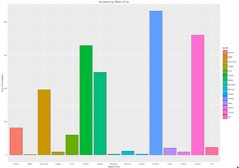
At this point we have written and tested our R code and know that it works.
3. Create a user defined R function and store it in the Oracle Database
Our next step in the process is to create an in-database user defined R function. This is were we store R code in our Oracle Database and make this available as an R function. To create the user defined R function we can use some PL/SQL to define it, and then take our R code (see above) and in it.
BEGIN
   -- sys.rqScriptDrop('demo_ggpplot');
   sys.rqScriptCreate('demo_ggpplot',
      'function(dat) {
         library(ggplot2)

         aggdata2 <- aggregate(dat$POLICYNUMBER,
                      by = list(MAKE = dat$MAKE),
                      FUN = length)

        g <-ggplot(data=aggdata2, aes(x=MAKE, y=x, fill=MAKE)) + geom_bar(color="black", stat="identity") +
                   xlab("Make of Car") + ylab("Num of Accidents") + ggtitle("Accidents by Make of Car")

        plot(g)
   }');
END;
We have to make a small addition to our R code. We need need to include a call to the plot function so that the image can be returned as a BLOB object. If you do not do this then the SQL query in step 4 will return no rows.
4. Write the SQL to call it
To call our defined R function we will need to use one of the ORE SQL API functions. In the following example we are using the rqTableEval function. The first parameter for this function passes in the data to be processed. In our case this is the data from the CLAIMS table. The second parameter is set to null. The third parameter is set to the output format and in our case we want this to be PNG. The fourth parameter is the name of the user defined R function.
select *
from table(rqTableEval( cursor(select * from claims),
                        null,
                        'PNG',
                        'demo_ggpplot'));
5. How to view the results
The SQL query in Step 4 above will return one row and this row will contain a column with a BLOB data type.

The easiest way to view the graphic that is produced is to use SQL Developer. It has an inbuilt feature that allows you to display BLOB objects. All you need to do is to double click on the BLOB cell (under the column labeled IMAGE). A window will open called ‘View Value’. In this window click the ‘View As Image’ check box on the top right hand corner of the window. When you do the R ggplot2 graphic will be displayed.

Yes the image is not 100% the same as the image produced in our R session. I will have another blog post that deals with this at a later date.
But, now you have written a SQL query, that calls R code to produce an R graphic (using ggplot2) of our data.
6. Now you can enhance the graphics (without changing your SQL)
What if you get bored with the bar chart and you want to change it to a different type of graphic? All you need to do is to change the relevant code in the user defined R function.
For example, if we want to change the graphic to a polar plot. The following is the PL/SQL code that re-defines the user defined R script.
BEGIN
   sys.rqScriptDrop('demo_ggpplot');
   sys.rqScriptCreate('demo_ggpplot',
      'function(dat) {
         library(ggplot2)

         aggdata2 <- aggregate(dat$POLICYNUMBER,
                      by = list(MAKE = dat$MAKE),
                      FUN = length)

         n <- nrow(aggdata2)
         degrees <- 360/n

        aggdata2$MAKE_ID <- 1:nrow(aggdata2)

        g<- ggplot(data=aggdata2, aes(x=MAKE, y=x, fill=MAKE)) + geom_bar(color="black", stat="identity") +
               xlab("Make of Car") + ylab("Num of Accidents") + ggtitle("Accidents by Make of Car") + coord_polar(theta="x")
        plot(g)
   }');
END;
We can use the exact same SQL query we defined in Step 4 above to call the next graphic.
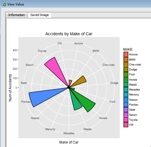
All done.
Now that was easy! Right?
I kind of is easy once you have been shown. There are a few challenges when working in-database user defined R functions and writing the SQL to call them. Most of the challenges are around the formatting of R code in the function and the syntax of the SQL statement to call it. With a bit of practice it does get easier.
7. Where/How can you use these graphics ?
Any application or program that can call and process a BLOB data type can display these images. For example, I’ve been able to include these graphics in applications developed in APEX.
Cluster Distance using SQL with Oracle Data Mining – Part 4
This is the fourth and last blog post in a series that looks at how you can examine the details of predicted clusters using Oracle Data Mining. In the previous blog posts I looked at how to use CLUSER_ID, CLUSTER_PROBABILITY and CLUSTER_SET.
In this blog post we will look at CLUSTER_DISTANCE. We can use the function to determine how close a record is to the centroid of the cluster. Perhaps we can use this to determine what customers etc we might want to focus on most. The customers who are closest to the centroid are one we want to focus on first. So we can use it as a way to prioritise our workflows, particularly when it is used in combination with the value for CLUSTER_PROBABILITY.
Here is an example of using CLUSTER_DISTANCE to list all the records that belong to Cluster 14 and the results are ordered based on closeness to the centroid of this cluster.
SELECT customer_id,
       cluster_probability(clus_km_1_37 USING *) as cluster_Prob,
       cluster_distance(clus_km_1_37 USING *) as cluster_Distance
FROM   insur_cust_ltv_sample
WHERE   cluster_id(clus_km_1_37 USING *) = 14
order by cluster_Distance asc;
Here is a subset of the results from this query.
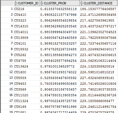
When you examine the results you may notice that the records that is listed first and closest record to the centre of cluster 14 has a very low probability. You need to remember that we are working in a N-dimensional space here. Although this first record is closest to the centre of cluster 14 it has a really low probability and if we examine this record in more detail we will find that it is at an overlapping point between a number of clusters.
This is why we need to use the CLUSTER_DISTANCE and CLUSTER_PROBABILITY functions together in our workflows and applications to determine how we need to process records like these.
Cluster Sets using SQL with Oracle Data Mining – Part 3
This is the third blog post on my series on examining the Clusters that were predicted by an Oracle Data Mining model. Check out the previous blog posts.
- Part 1 – Examining predicted Clusters and Cluster details using SQL
- Part 2 – Cluster Details with Oracle Data Mining
In the previous posts we were able to list the predicted cluster for each record in our data set. This is the cluster that the records belonged to the most. I also mentioned that a record could belong to many clusters.
So how can you list all the clusters that the a record belongs to?
You can use the CLUSTER_SET SQL function. This will list the Cluster Id and a probability measure for each cluster. This function returns a array consisting of the set of all clusters that the record belongs to.
The following example illustrates how to use the CLUSTER_SET function for a particular cluster model.
SELECT t.customer_id, s.cluster_id, s.probability
FROM   (select customer_id, cluster_set(clus_km_1_37 USING *) as Cluster_Set
        from   insur_cust_ltv_sample
        WHERE  customer_id in ('CU13386', 'CU100')) T,
      TABLE(T.cluster_set) S
order by t.customer_id, s.probability desc;
The output from this query will be an ordered data set based on the customer id and then the clusters listed in descending order of probability. The cluster with the highest probability is what would be returned by the CLUSTER_ID function. The output from the above query is shown below.

If you would like to see the details of each of the clusters and to examine the differences between these clusters then you will need to use the CLUSTER_DETAILS function (see previous blog post).
You can specify topN and cutoff to limit the number of clusters returned by the function. By default, both topN and cutoff are null and all clusters are returned.
– topN is the N most probable clusters. If multiple clusters share the Nth probability, then the function chooses one of them.
– cutoff is a probability threshold. Only clusters with probability greater than or equal to cutoff are returned. To filter by cutoff only, specify NULL for topN.
You may want to use these individually or combined together if you have a large number of customers. To return up to the N most probable clusters that are greater than or equal to cutoff, specify both topN and cutoff.
The following example illustrates using the topN value to return the top 4 clusters.
SELECT t.customer_id, s.cluster_id, s.probability
FROM   (select customer_id, cluster_set(clus_km_1_37, 4, null USING *) as Cluster_Set
        from   insur_cust_ltv_sample
        WHERE  customer_id in ('CU13386', 'CU100')) T,
      TABLE(T.cluster_set) S
order by t.customer_id, s.probability desc;
and the output from this query shows only 4 clusters displayed for each record.

Alternatively you can select the clusters based on a cut off value for the probability. In the following example this is set to 0.05.
SELECT t.customer_id, s.cluster_id, s.probability
FROM   (select customer_id, cluster_set(clus_km_1_37, NULL, 0.05 USING *) as Cluster_Set
        from   insur_cust_ltv_sample
        WHERE  customer_id in ('CU13386', 'CU100')) T,
      TABLE(T.cluster_set) S
order by t.customer_id, s.probability desc;
and the output this time looks a bit different.

Finally, yes you can combine these two parameters to work together.
SELECT t.customer_id, s.cluster_id, s.probability
FROM (select customer_id, cluster_set(clus_km_1_37, 2, 0.05 USING *) as Cluster_Set
from insur_cust_ltv_sample
WHERE customer_id in (‘CU13386’, ‘CU100’)) T,
TABLE(T.cluster_set) S
order by t.customer_id, s.probability desc;
Examining predicted Clusters and Cluster details using SQL
In a previous blog post I gave some details of how you can examine some of the details behind a prediction made using a classification model. This seemed to spark a lot of interest. But before I come back to looking at classification prediction details and other information, this blog post is the first in a 4 part blog post on examining the details of Clusters, as identified by a cluster model created using Oracle Data Mining.
The 4 blog posts will consist of:
- 1 – (this blog post) will look at how to determine the predicted cluster and cluster probability for your record.
- 2 – will show you how to examine the details behind and used to predict the cluster.
- 3 – A record could belong to many clusters. In this blog post we will look at how you can determine what clusters a record can belong to.
- 4 – Cluster distance is a measure of how far the record is from the cluster centroid. As a data point or record can belong to many clusters, it can be useful to know the distances as you can build logic to perform different actions based on the cluster distances and cluster probabilities.
Right. Let’s have a look at the first set of these closer functions. These are CLUSTER_ID and CLUSTER_PROBABILITY.
CLUSER_ID : Returns the number of the cluster that the record most closely belongs to. This is measured by the cluster distance to the centroid of the cluster. A data point or record can belong or be part of many clusters. So the CLUSTER_ID is the cluster number that the data point or record most closely belongs too.
CLUSTER_PROBABILITY : Is a probability measure of the likelihood of the data point or record belongs to a cluster. The cluster with the highest probability score is the cluster that is returned by the CLUSTER_ID function.
Now let us have a quick look at the SQL for these two functions. This first query returns the cluster number that each record most strong belongs too.
SELECT customer_id,
       cluster_id(clus_km_1_37 USING *) as Cluster_Id,
FROM   insur_cust_ltv_sample
WHERE  customer_id in ('CU13386', 'CU6607', 'CU100');

Now let us add in the cluster probability function.
SELECT customer_id,
       cluster_id(clus_km_1_37 USING *) as Cluster_Id,
       cluster_probability(clus_km_1_37 USING *) as cluster_Prob
FROM   insur_cust_ltv_sample
WHERE  customer_id in ('CU13386', 'CU6607', 'CU100');
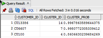
These functions gives us some insights into what the cluster predictive model is doing. In the remaining blog posts in this series I will look at how you can delve deeper into the predictions that the cluster algorithm is make.
PREDICTION_DETAILS function in Oracle
When building predictive models the data scientist can spend a large amount of time examining the models produced and how they work and perform on their hold out sample data sets. They do this to understand is the model gives a good general representation of the data and can identify/predict many different scenarios. When the “best” model has been selected then this is typically deployed is some sort of reporting environment, where a list is produced. This is typical deployment method but is far from being ideal. A more ideal deployment method is that the predictive models are build into the everyday applications that the company uses. For example, it is build into the call centre application, so that the staff have live and real-time feedback and predictions as they are talking to the customer.
But what kind of live and real-time feedback and predictions are possible. Again if we look at what is traditionally done in these applications they will get a predicted outcome (will they be a good customer or a bad customer) or some indication of their value (maybe lifetime value, possible claim payout value) etc.
But can we get anymore information? Information like what was reason for the prediction. This is sometimes called prediction insight. Can we get some details of what the prediction model used to decide on the predicted value. In more predictive analytics products this is not possible, as all you are told is the final out come.
What would be useful is to know some of the thinking that the predictive model used to make its thinking. The reasons when one customer may be a “bad customer” might be different to that of another customer. Knowing this kind of information can be very useful to the staff who are dealing with the customers. For those who design the workflows etc can then build more advanced workflows to support the staff when dealing with the customers.
Oracle as a unique feature that allows us to see some of the details that the prediction model used to make the prediction. This functions (based on using the Oracle Advanced Analytics option and Oracle Data Mining to build your predictive model) is called PREDICTION_DETAILS.
When you go to use PREDICTION_DETAILS you need to be careful as it will work differently in the 11.2g and 12c versions of the Oracle Database (Enterprise Editions). In Oracle Database 11.2g the PREDICTION_DETAILS function would only work for Decision Tree models. But in 12c (and above) it has been opened to include details for models created using all the classification algorithms, all the regression algorithms and also for anomaly detection.
The following gives an example of using the PREDICTION_DETAILS function.
select cust_id,
       prediction(clas_svm_1_27 using *) pred_value,
       prediction_probability(clas_svm_1_27 using *) pred_prob,
       prediction_details(clas_svm_1_27 using *) pred_details
from mining_data_apply_v;
The PREDICTION_DETAILS function produces its output in XML, and this consists of the attributes used and their values that determined why a record had the predicted value. The following gives some examples of the XML produced for some of the records.
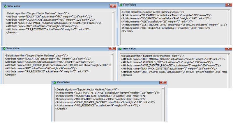
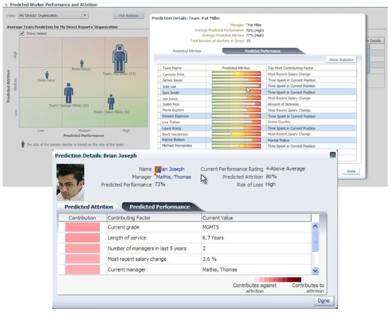
I’ve used this particular function in lots of my projects and particularly when building the applications for a particular business unit. Oracle too has build this functionality into many of their applications. The images below are from the HCM application where you can examine the details why an employee may or may not leave/churn. You can when perform real-time what-if analysis by changing some of attribute values to see if the predicted out come changes.
Accessing the R datasets in ORE and SQL
When you install R you also get a set of pre-compiled datasets. These are great for trying out many of the features that are available with R and all the new packages that are being produced on an almost daily basis.
The exact list of data sets available will depend on the version of R that you are using.
To get the list of available data sets in R you can run the following.
> library(help="datasets")
This command will list all the data sets that you can reference and start using immediately.
I’m currently running the latest version of Oracle R Distribution version 3.2. See the listing at the end of this blog post for the available data sets.
But are these data sets available to you if you are using Oracle R Enterprise (ORE)? The answer is Yes of course they are.
But are these accessible on the Oracle Database server? Yes they are, as you have R installed there and you can use ORE to access and use the data sets.
But how? how can I list what is on the Oracle Database server using R? Simple use the following ORE code to run an embedded R execution function using the ORE R API.
What? What does that mean? Using the R on your client machine, you can use ORE to send some R code to the Oracle Database server. The R code will be run on the Oracle Database server and the results will be returned to the client. The results contain the results from the server. Try the following code.
ore.doEval(function() library(help="datasets"))

# let us create a functions for this code
myFn <- function() {library(help="datasets")}

# Now send this function to the DB server and run it there.
ore.doEval(myFn)

# create an R script in the Oracle Database that contains our R code
ore.scriptDrop("inDB_R_DemoData")
ore.scriptCreate("inDB_R_DemoData", myFn)
# Now run the R script, stored in the Oracle Database, on the Database server
#   and return the results to my client
ore.doEval(FUN.NAME="inDB_R_DemoData")
Simple, Right!
Yes it is. You have shown us how to do this in R using the ORE package. But what if I’m a SQL developer. Can I do this in SQL? Yes you can. Connect you your schema using SQL Developer/SQL*Plus/SQLcl or whatever tool you will be using to run SQL. Then run the following SQL.
select *
from table(rqEval(null, 'XML', 'inDB_R_DemoData'));
This SQL code will return the results in XML format. You can parse this to extract and display the results and when you do you will get something like the following listing, which is exactly the same that is produced when you run the R code that I gave above.
So what this means is that evening if you have an empty schema with no data in it, and as long as you have the privileges to run embedded R execution, you actually have access to all these different data sets. You can use these to try our R using the ORE SQL APIs too.
		Information on package ‘datasets’

Description:

Package:       datasets
Version:       3.2.0
Priority:      base
Title:         The R Datasets Package
Author:        R Core Team and contributors worldwide
Maintainer:    R Core Team
Description:   Base R datasets.
License:       Part of R 3.2.0
Built:         R 3.2.0; ; 2015-08-07 02:20:26 UTC; windows

Index:

AirPassengers           Monthly Airline Passenger Numbers 1949-1960
BJsales                 Sales Data with Leading Indicator
BOD                     Biochemical Oxygen Demand
CO2                     Carbon Dioxide Uptake in Grass Plants
ChickWeight             Weight versus age of chicks on different diets
DNase                   Elisa assay of DNase
EuStockMarkets          Daily Closing Prices of Major European Stock
                        Indices, 1991-1998
Formaldehyde            Determination of Formaldehyde
HairEyeColor            Hair and Eye Color of Statistics Students
Harman23.cor            Harman Example 2.3
Harman74.cor            Harman Example 7.4
Indometh                Pharmacokinetics of Indomethacin
InsectSprays            Effectiveness of Insect Sprays
JohnsonJohnson          Quarterly Earnings per Johnson & Johnson Share
LakeHuron               Level of Lake Huron 1875-1972
LifeCycleSavings        Intercountry Life-Cycle Savings Data
Loblolly                Growth of Loblolly pine trees
Nile                    Flow of the River Nile
Orange                  Growth of Orange Trees
OrchardSprays           Potency of Orchard Sprays
PlantGrowth             Results from an Experiment on Plant Growth
Puromycin               Reaction Velocity of an Enzymatic Reaction
Theoph                  Pharmacokinetics of Theophylline
Titanic                 Survival of passengers on the Titanic
ToothGrowth             The Effect of Vitamin C on Tooth Growth in
                        Guinea Pigs
UCBAdmissions           Student Admissions at UC Berkeley
UKDriverDeaths          Road Casualties in Great Britain 1969-84
UKLungDeaths            Monthly Deaths from Lung Diseases in the UK
UKgas                   UK Quarterly Gas Consumption
USAccDeaths             Accidental Deaths in the US 1973-1978
USArrests               Violent Crime Rates by US State
USJudgeRatings          Lawyers' Ratings of State Judges in the US
                        Superior Court
USPersonalExpenditure   Personal Expenditure Data
VADeaths                Death Rates in Virginia (1940)
WWWusage                Internet Usage per Minute
WorldPhones             The World's Telephones
ability.cov             Ability and Intelligence Tests
airmiles                Passenger Miles on Commercial US Airlines,
                        1937-1960
airquality              New York Air Quality Measurements
anscombe                Anscombe's Quartet of 'Identical' Simple Linear
                        Regressions
attenu                  The Joyner-Boore Attenuation Data
attitude                The Chatterjee-Price Attitude Data
austres                 Quarterly Time Series of the Number of
                        Australian Residents
beavers                 Body Temperature Series of Two Beavers
cars                    Speed and Stopping Distances of Cars
chickwts                Chicken Weights by Feed Type
co2                     Mauna Loa Atmospheric CO2 Concentration
crimtab                 Student's 3000 Criminals Data
datasets-package        The R Datasets Package
discoveries             Yearly Numbers of Important Discoveries
esoph                   Smoking, Alcohol and (O)esophageal Cancer
euro                    Conversion Rates of Euro Currencies
eurodist                Distances Between European Cities and Between
                        US Cities
faithful                Old Faithful Geyser Data
freeny                  Freeny's Revenue Data
infert                  Infertility after Spontaneous and Induced
                        Abortion
iris                    Edgar Anderson's Iris Data
islands                 Areas of the World's Major Landmasses
lh                      Luteinizing Hormone in Blood Samples
longley                 Longley's Economic Regression Data
lynx                    Annual Canadian Lynx trappings 1821-1934
morley                  Michelson Speed of Light Data
mtcars                  Motor Trend Car Road Tests
nhtemp                  Average Yearly Temperatures in New Haven
nottem                  Average Monthly Temperatures at Nottingham,
                        1920-1939
npk                     Classical N, P, K Factorial Experiment
occupationalStatus      Occupational Status of Fathers and their Sons
precip                  Annual Precipitation in US Cities
presidents              Quarterly Approval Ratings of US Presidents
pressure                Vapor Pressure of Mercury as a Function of
                        Temperature
quakes                  Locations of Earthquakes off Fiji
randu                   Random Numbers from Congruential Generator
                        RANDU
rivers                  Lengths of Major North American Rivers
rock                    Measurements on Petroleum Rock Samples
sleep                   Student's Sleep Data
stackloss               Brownlee's Stack Loss Plant Data
state                   US State Facts and Figures
sunspot.month           Monthly Sunspot Data, from 1749 to "Present"
sunspot.year            Yearly Sunspot Data, 1700-1988
sunspots                Monthly Sunspot Numbers, 1749-1983
swiss                   Swiss Fertility and Socioeconomic Indicators
                        (1888) Data
treering                Yearly Treering Data, -6000-1979
trees                   Girth, Height and Volume for Black Cherry Trees
uspop                   Populations Recorded by the US Census
volcano                 Topographic Information on Auckland's Maunga
                        Whau Volcano
warpbreaks              The Number of Breaks in Yarn during Weaving
women                   Average Heights and Weights for American Women
Oracle Advanced Analytics in the Oracle Cloud
You have heard about the cloud? Right? Even the Oracle Cloud?
If you haven’t, then maybe we need to look at how you can learn more about the Oracle Cloud.
Over the past while, and in the past few weeks in particular, Oracle has been advertising about how you can get a trail Oracle cloud service setup for FREE. Well it is free for one month when you set it up on the Oracle website (cloud.oracle.com).
As I like to talk about and use the Oracle Advanced Analytics (OAA) option (a lot), I thought I’d just give you some pointers on how to use OAA on the Oracle cloud.
To do this you need to set up an account on the Oracle cloud website (your Oracle single sign on should help with making that process a lot quicker). There are lots of websites and blog that will talk/show you through the process. Then you need to select what Database as a Service that you want to setup
OAA is not available on the Database Schema Service just yet (maybe one day they will)
Although Oracle Advanced Analytics comes pre-installed in the Oracle Enterprise Edition database (yes it is a separately priced option) when you install it on your own servers, but for the Enterprise Edition DaaS OAA is not part of it.
DaaS has the following versions
- Standard Edition Service
- Enterprise Edition Service
- High Performance Service
- Extreme Performance Service
OAA is only available for these last two versions of the DaaS.
High Performance DaaS: Multitenant, Partitioning, Real Application Testing, Advanced Compression, Advanced Security, Label Security, Database Vault, OLAP, Advanced Analytics, Spatial and Graph, Diagnostics Pack, Tuning Pack, Database Lifecycle Management Pack, Data Masking & Subsetting Pack and Cloud Management Pack for Oracle Database.
Extreme Performance DaaS: In-Memory Database, RAC (Real Application Clusters), Active Data Guard, Multitenant, Partitioning, Real Application Testing, Advanced Compression, Advanced Security, Label Security, Database Vault, OLAP, Advanced Analytics, Spatial and Graph, Diagnostics Pack, Tuning Pack, Database Lifecycle Management Pack, Data Masking & Subsetting Pack and Cloud Management Pack for Oracle Database.
Oracle Advanced Analytics has two main products or components. The first is the in-database Oracle Data Mining features. This are part of the High Performance and Extreme Performance DaaS offerings. But Oracle R Enterprise is not installed on these DaaS. Well if kind of is if you can get an 11g DaaS, but at time of writing this post ORE is not part of the 12c DaaS images. So you will need to factor in some time to go and install ORE, if you need to use it.
I’ve been lucky to have one of these DaaS with OAA trials and with thanks to Thomas Kurian he has extended these trials to 12 months for all Oracle ACE Directors. Thank you Thomas.
When you get your DaaS setup you just need to configure your connection privileges, ssh, etc and away you go. All you need to do is to move your data across the internet to your own Oracle DaaS, and once it is in the DaaS all your OAA and other analytics is performed on the Database Server. Only the results are returned to you and displayed in your tool. This significantly reduces the processing time for your data and removes the need to constantly extract your data (in whole or in parts) to feed into other advanced analytics tools.
So if you haven’t tried Oracle Advanced Analytics yet, then go ahead and setup your free trial of Oracle DaaS and try it out. You never know what you might discover by using Oracle Advanced Analytics (in the cloud)

- ← Previous
- 1
- 2
