
RandomForest
Combining NLP and Machine Learning for Document Classification
Text mining is a popular topic for exploring what text you have in documents etc. Text mining and NLP can help you discover different patterns in the text like uncovering certain words or phases which are commonly used, to identifying certain patterns and linkages between different texts/documents. Combining this work on Text mining you can use Word Clouds, time-series analysis, etc to discover other aspects and patterns in the text. Check out my previous blog posts (post 1, post 2) on performing Text Mining on documents (manifestos from some of the political parties from the last two national government elections in Ireland). These two posts gives you a simple indication of what is possible.
We can build upon these Text Mining examples to include other machine learning algorithms like those for Classification. With Classification we want to predict or label a record or document to have a particular value. With Classification this could involve labeling a document as being positive or negative (movie or book reviews), or determining if a document is for a particular domain such as Technology, Sports, Entertainment, etc
With Classification problems we typically have a case record containing many different feature/attributes. You will see many different examples of this. When we add in Text Mining we are adding new/additional features/attributes to the case record. These new features/attributes contain some characteristics of the Word (or Term) frequencies in the documents. This is a form of feature engineering, where we create new features/attributes based on our dataset.
Let’s work through an example of using Text Mining and Classification Algorithm to build a model for determining/labeling/classifying documents.
The Dataset: For this example I’ll use Move Review dataset from Cornell University. Download and unzip the file. This will create a set of directories with the reviews (as individual documents) listed under the ‘pos’ or ‘neg’ directory. This dataset contains approximately 2000 documents. Other datasets you could use include the Amazon Reviews or the Disaster Tweets.
The following is the Python code to perform NLP to prepare the data, build a classification model and test this model against a holdout dataset. First thing is to load the libraries NLP and some other basics.
import numpy as np
import re
import nltk
from sklearn.datasets import load_files
from nltk.corpus import stopwords
Load the dataset.
#This dataset will allow use to perform a type of Sentiment Analysis Classification
source_file_dir = r"/Users/brendan.tierney/Dropbox/4-Datasets/review_polarity/txt_sentoken"

#The load_files function automatically divides the dataset into data and target sets.
#load_files  will treat each folder inside the "txt_sentoken" folder as one category
#  and all the documents inside that folder will be assigned its corresponding category.
movie_data = load_files(source_file_dir)
X, y = movie_data.data, movie_data.target

#load_files  function loads the data from both "neg" and "pos" folders into the X variable,
#  while the target categories are stored in y
We can now use the typical NLP tasks on this data. This will clean the data and prepare it.
documents = []
documents = []

from nltk.stem import WordNetLemmatizer

stemmer = WordNetLemmatizer()

for sen in range(0, len(X)):
    # Remove all the special characters, numbers, punctuation
    document = re.sub(r'\W', ' ', str(X[sen]))

    # remove all single characters
    document = re.sub(r'\s+[a-zA-Z]\s+', ' ', document)

    # Remove single characters from the start of document with a space
    document = re.sub(r'\^[a-zA-Z]\s+', ' ', document)

    # Substituting multiple spaces with single space
    document = re.sub(r'\s+', ' ', document, flags=re.I)

    # Removing prefixed 'b'
    document = re.sub(r'^b\s+', '', document)

    # Converting to Lowercase
    document = document.lower()

    # Lemmatization
    document = document.split()

    document = [stemmer.lemmatize(word) for word in document]
    document = ' '.join(document)

    documents.append(document)
You can see we have removed all special characters, numbers, punctuation, single characters, spacing, special prefixes, converted all words to lower case and finally extracted the stemmed word.
Next we need to take these words and convert them into numbers, as the algorithms like to work with numbers rather then text. One particular approach is Bag of Words.
The first thing we need to decide on is the maximum number of words/features to include or use for later stages. As you can image when looking across lots and lots of documents you will have a very large number of words. Some of these are repeated words. What we are interested in are frequently occurring words, which means we can ignore low frequently occurring works. To do this we can set max_feature to a defined value. In our example we will set it to 1500, but in your problems/use cases you might need to experiment to determine what might be a better values.
Two other parameters we need to set include min_df and max_df. min_df sets the minimum number of documents to contain the word/feature. max_df specifies the percentage of documents where the words occur, for example if this is set to 0.7 this means the words should occur in a maximum of 70% of the documents.
from sklearn.feature_extraction.text import CountVectorizer
vectorizer = CountVectorizer(max_features=1500, min_df=5, max_df=0.7,stop_words=stopwords.words('english'))
X = vectorizer.fit_transform(documents).toarray()
The CountVectorizer in the above code also remove Stop Words for the English language. These words are generally basic words that do not convey any meaning. You can easily add to this list and adjust it to suit your needs and to reflect word usage and meaning for your particular domain.
The bag of words approach works fine for converting text to numbers. However, it has one drawback. It assigns a score to a word based on its occurrence in a particular document. It doesn’t take into account the fact that the word might also be having a high frequency of occurrence in other documentsas well. TFIDF resolves this issue by multiplying the term frequency of a word by the inverse document frequency. The TF stands for “Term Frequency” while IDF stands for “Inverse Document Frequency”.
And the Inverse Document Frequency is calculated as:
IDF(word) = Log((Total number of documents)/(Number of documents containing the word))
The term frequency is calculated as:
Term frequency = (Number of Occurrences of a word)/(Total words in the document)
The TFIDF value for a word in a particular document is higher if the frequency of occurrence of thatword is higher in that specific document but lower in all the other documents.
To convert values obtained using the bag of words model into TFIDF values, run the following:
from sklearn.feature_extraction.text import TfidfTransformer
tfidfconverter = TfidfTransformer()
X = tfidfconverter.fit_transform(X).toarray()
That’s the dataset prepared, the final step is to create the Training and Test datasets.
from sklearn.model_selection import train_test_split
X_train, X_test, y_train, y_test = train_test_split(X, y, test_size=0.2, random_state=0)
#Train DS = 70%
#Test DS = 30%
There are several machine learning algorithms you can use. These are the typical classification algorithms. But for simplicity I’m going to use RandomForest algorithm in the following code. After giving this a go, try to do it for the other algorithms and compare the results.
#Import Random Forest Model
#Use RandomForest algorithm to create a model
#n_estimators = number of trees in the Forest

from sklearn.ensemble import RandomForestClassifier
classifier = RandomForestClassifier(n_estimators=1000, random_state=0)
classifier.fit(X_train, y_train)
Now we can test the model on the hold-out or Test dataset
#Now label/classify the Test DS
y_pred = classifier.predict(X_test)

#Evaluate the model
from sklearn.metrics import classification_report, confusion_matrix, accuracy_score

print("Accuracy:", accuracy_score(y_test, y_pred))
print(confusion_matrix(y_test,y_pred))
print(classification_report(y_test,y_pred))
This model gives the following results, with an over all accuracy of 85% (you might get a slightly different figure). This is a good outcome and a good predictive model. But is it the best one? We simply don’t know at this point. Using the ‘No Free Lunch Theorem’ we would would have to see what results we would get from the other algorithms.
Although this example only contains the words from the documents, we can see how we could include this with other features/attributes when forming a case record. For example, our case records represented Insurance Claims, the features would include details of the customer, their insurance policy, the amount claimed, etc and in addition could include incident reports, claims assessor reports etc. This would be documents which we can include in the building a predictive model to determine of an insurance claim is fraudulent or not.
RandomForest Machine Learning – Oracle Machine Learning (OML)
Oracle Machine Learning has 30+ different machine learning algorithms built into the database. This means you can use SQL to create machine learning models and then use these models to score or label new data stored in the database or as the data is being created dynamically in the applications.
One of the most commonly used machine learning algorithms, over the past few years, is can RandomForest. This post will take a closer look at this algorithm and how you can build & use a RandomForest model.
Random Forest is known as an ensemble machine learning technique that involves the creation of hundreds of decision tree models. These hundreds of models are used to label or score new data by evaluating each of the decision trees and then determining the outcome based on the majority result from all the decision trees. Just like in the game show. The combining of a number of different ways of making a decision can result in a more accurate result or prediction.
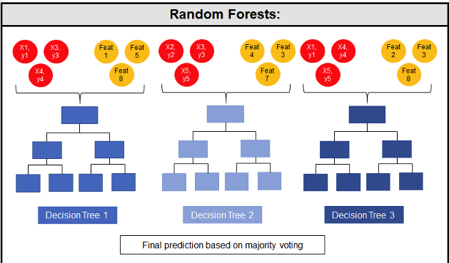
Random Forest models can be used for classification and regression types of problems, which form the majority of machine learning systems and solutions. For classification problems, this is where the target variable has either a binary value or a small number of defined values. For classification problems the Random Forest model will evaluate the predicted value for each of the decision trees in the model. The final predicted outcome will be the majority vote for all the decision trees. For regression problems the predicted value is numeric and on some range or scale. For example, we might want to predict a customer’s lifetime value (LTV), or the potential value of an insurance claim, etc. With Random Forest, each decision tree will make a prediction of this numeric value. The algorithm will then average these values for the final predicted outcome.
Under the hood, Random Forest is a collection of decision trees. Although decision trees are a popular algorithm for machine learning, they can have a tendency to over fit the model. This can lead higher than expected errors when predicting unseen data. It also gives just one possible way of representing the data and being able to derive a possible predicted outcome.
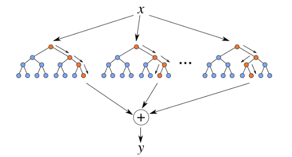 Random Forest on the other hand relies of the predicted outcomes from many different decision trees, each of which is built in a slightly different way. It is an ensemble technique that combines the predicted outcomes from each decision tree to give one answer. Typically, the number of trees created by the Random Forest algorithm is defined by a parameter setting, and in most languages this can default to 100+ or 200+ trees.
The Random Forest algorithm has three main features:
- It uses a method called bagging to create different subsets of the original training data
- It will randomly section different subsets of the features/attributes and build the decision tree based on this subset
- By creating many different decision trees, based on different subsets of the training data and different subsets of the features, it will increase the probability of capturing all possible ways of modeling the data
For each decision tree produced, the algorithm will use a measure, such as the Gini Index, to select the attributes to split on at each node of the decision tree.
To create a RandomForest model using Oracle Data Mining, you will follow the same process as with any of the other algorithms, the core of these are:
- define the parameter settings
- create the model
- score/label new data
Let’s start with the first step, defining the parameters. As with all the classification algorithms the same or similar parameters are set. With RandomForest we can set an additional parameter which tells the algorithm how many decision trees to create as part of the model. By default, 20 decision trees will be created. But if you want to change this number you can use the RFOR_NUM_TREES parameter. Remember the larger the value the longer it will take to create the model. But will have better accuracy. On the other hand with a small number of trees the quicker the model build will be, but might night be as accurate. This is something you will need to explore and determine. In the following example I change the number of trees to created to ten.
CREATE TABLE BANKING_RF_SETTINGS (
    SETTING_NAME VARCHAR2(50),
    SETTING_VALUE VARCHAR2(50)
);

BEGIN
  DELETE FROM BANKING_RF_SETTINGS;

  INSERT INTO banking_RF_settings (setting_name, setting_value)
  VALUES (dbms_data_mining.algo_name, dbms_data_mining.algo_random_forest);

  INSERT INTO banking_RF_settings (setting_name, setting_value)
  VALUES (dbms_data_mining.prep_auto, dbms_data_mining.prep_auto_on);

  INSERT INTO banking_RF_settings (setting_name, setting_value)
  VALUES (dbms_data_mining.RFOR_NUM_TREES, 10);

  COMMIT;
END;
Other default parameters used include, for creating each decision tree, use random 50% selection of columns and 50% sample of training data.
Now for step 2, create the model.
DECLARE
   v_start_time  TIMESTAMP;
BEGIN
   DBMS_DATA_MINING.DROP_MODEL('BANKING_RF_72K_1');

   v_start_time := current_timestamp;

   DBMS_DATA_MINING.CREATE_MODEL(
      model_name          => 'BANKING_RF_72K_1',
      mining_function     => dbms_data_mining.classification,
      data_table_name     => 'BANKING_72K',
      case_id_column_name => 'ID',
      target_column_name  => 'TARGET',
      settings_table_name => 'BANKING_RF_SETTINGS');

   dbms_output.put_line('Time take to create model = ' || to_char(extract(second from (current_timestamp-v_start_time))) || ' seconds.');
END;
The above code measures how long it takes to create the model.
I’ve run this same parameters and create models for different training data set sizes. I’ve also changed the number of decision trees to create. The following table shows the timings.
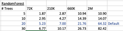
You can see it took 5.23 seconds to create a RandomForest model using the default settings for a data set of 72K records. This increase to just over one minute for a data set of 2 million records. Yo can also see the effect of reducing the number of decision trees on how long it takes the create model to run.
For step 3, on using the model on new data, this is just the same as with any of the classification models. Here is an example:
SELECT cust_id, target,
       prediction(BANKING_RF_72K_1 USING *)  predicted_value,
       prediction_probability(BANKING_RF_72K_1 USING *) probability
FROM   bank_test_v;
That’s it. That’s all there is to creating a RandomForest machine learning model using Oracle Machine Learning.
It’s quick and easy 🙂

You must be logged in to post a comment.