
python-oracledb driver version 3 – load data into pandas df
The Python Oracle driver had a new release recently (version 3) and with it comes a new way to load data from a Table into a Pandas dataframe. This can now be done using the pyarrow library. Here’s an example:
import oracledb ora
import pyarrow py
import pandas

#create a connection to the database
con = ora.connect( <enter your connection details> )

query = "select cust_id, cust_first_name, cust_last_name, cust_city from customers"

#get Oracle DF and set array size - care is needed for setting this
ora_df = con.fetch_df_all(statement=query, arraysize=2000)

#run query and return into Pandas Dataframe
#  using pyarrow and the to_pandas() function
df = py.Table.from_arrays(ora_df.column_arrays(), names=ora_df.columns()).to_pandas()

print(df.columns)
Once you get used to the syntax it is a simpler way to get the data into dataframe.
BOCAS – using OCI GenAI Agent and Stremlit
BOCAS stands for Brendan’s Oracle Chatbot Agent for Shakespeare. I’ve previously posted on how to go about creating a GenAI Agent on a specific data set. In this post, I’ll share code on how I did this using Python Streamlit.
And here’s the code
import streamlit as st
import time
import oci
from oci import generative_ai_agent_runtime
import json
# Page Title
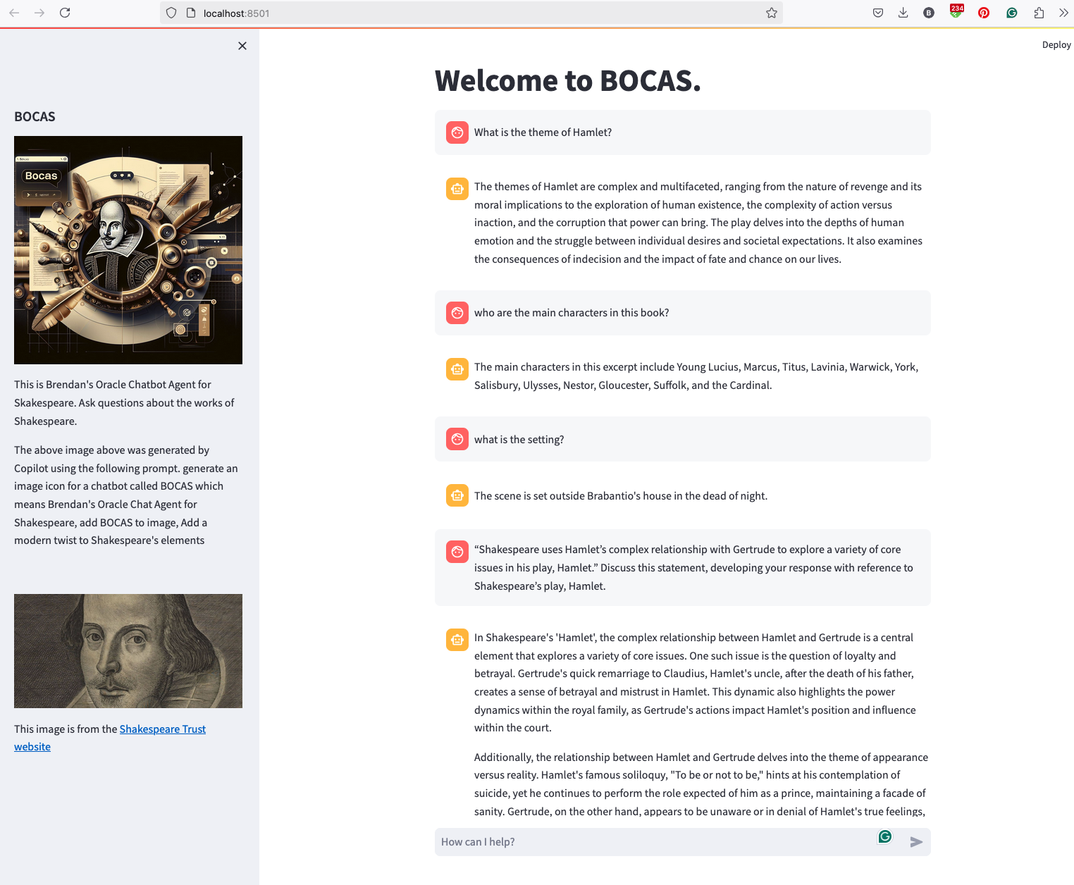
welcome_msg = "Welcome to BOCAS."
welcome_msg2 = "This is Brendan's Oracle Chatbot Agent for Skakespeare. Ask questions about the works of Shakespeare."
st.title(welcome_msg)
# Sidebar Image
st.sidebar.header("BOCAS")
st.sidebar.image("bocas-3.jpg", use_column_width=True)
#with st.sidebar:
# with st.echo:
# st.write(welcome_msg2)
st.sidebar.markdown(welcome_msg2)
st.sidebar.markdown("The above image above was generated by Copilot using the following prompt. generate an image icon for a chatbot called BOCAS which means Brendan's Oracle Chat Agent for Shakespeare, add BOCAS to image, Add a modern twist to Shakespeare's elements")
st.sidebar.write("")
st.sidebar.write("")
st.sidebar.write("")
st.sidebar.image("https://media.shakespeare.org.uk/images/SBT_SR_OS_37_Shakespeare_Firs.ec42f390.fill-1200x600-c75.jpg")
link="This image is from the [Shakespeare Trust website](https://media.shakespeare.org.uk/images/SBT_SR_OS_37_Shakespeare_Firs.ec42f390.fill-1200x600-c75.jpg)"
st.sidebar.write(link,unsafe_allow_html=True)
# OCI GenAI settings
CONFIG_PROFILE = "DEFAULT"
config = oci.config.from_file('~/.oci/config', CONFIG_PROFILE)
###
SERVICE_EP = <your service endpoint>
AGENT_EP_ID = <your agent endpoint>
###
# Response Generator
def response_generator(text_input):
#Initiate AI Agent runtime client
genai_agent_runtime_client = generative_ai_agent_runtime.GenerativeAiAgentRuntimeClient(config, service_endpoint=SERVICE_EP, retry_strategy=oci.retry.NoneRetryStrategy())
create_session_details = generative_ai_agent_runtime.models.CreateSessionDetails()
create_session_details.display_name = "Welcome to BOCAS"
create_session_details.idle_timeout_in_seconds = 20
create_session_details.description = welcome_msg
create_session_response = genai_agent_runtime_client.create_session(create_session_details, AGENT_EP_ID)
#Define Chat details and input message/question
session_details = generative_ai_agent_runtime.models.ChatDetails()
session_details.session_id = create_session_response.data.id
session_details.should_stream = False
session_details.user_message = text_input
#Get AI Agent Respose
session_response = genai_agent_runtime_client.chat(agent_endpoint_id=AGENT_EP_ID, chat_details=session_details)
#print(str(response.data))
response = session_response.data.message.content.text
return response
# Initialize chat history
if "messages" not in st.session_state:
st.session_state.messages = []
# Display chat messages from history on app rerun
for message in st.session_state.messages:
with st.chat_message(message["role"]):
st.markdown(message["content"])
# Accept user input
if prompt := st.chat_input("How can I help?"):
# Add user message to chat history
st.session_state.messages.append({"role": "user", "content": prompt})
# Display user message in chat message container
with st.chat_message("user"):
st.markdown(prompt)
# Display assistant response in chat message container
with st.chat_message("assistant"):
response = response_generator(prompt)
write_response = st.write(response)
st.session_state.messages.append({"role": "ai", "content": response})
# Add assistant response to chat historyCalling Custom OCI Gen AI Agent using Python
In a previous post, I demonstrated how to create a custom Generative AI Agent on OCI. This GenAI Agent was built using some of Shakespeare’s works. Using the OCI GenAI Agent interface is an easy way to test the Agent and to see how it behaves. Beyond that, it doesn’t have any use as you’ll need to call it using some other language or tool. The most common of these is using Python.
The code below calls my GenAI Agent, which I’ve called BOCAS (Brendan’s Oracle Chat Agent for Shakespeare).
import oci
from oci import generative_ai_agent_runtime
import json
from colorama import Fore, Back, Style
CONFIG_PROFILE = "DEFAULT"
config = oci.config.from_file('~/.oci/config', CONFIG_PROFILE)
#AI Agent service endpoint
SERVICE_EP = <add your Service Endpoint>
AGENT_EP_ID = <add your GenAI Agent Endpoint>
welcome_msg = "This is Brendan's Oracle Chatbot Agent for Shakespeare. Ask questions about the works of Shakespeare."
def gen_Agent_Client():
#Initiate AI Agent runtime client
genai_agent_runtime_client = generative_ai_agent_runtime.GenerativeAiAgentRuntimeClient(config, service_endpoint=SERVICE_EP, retry_strategy=oci.retry.NoneRetryStrategy())
create_session_details = generative_ai_agent_runtime.models.CreateSessionDetails()
create_session_details.display_name = "Welcome to BOCAS"
create_session_details.idle_timeout_in_seconds = 20
create_session_details.description = welcome_msg
return create_session_details, genai_agent_runtime_client
def Quest_Answer(user_question, create_session_details, genai_agent_runtime_client):
#Create a Chat Session for AI Agent
try:
create_session_response = genai_agent_runtime_client.create_session(create_session_details, AGENT_EP_ID)
except:
create_session_details, genai_agent_runtime_client = gen_Agent_Client()
create_session_response = genai_agent_runtime_client.create_session(create_session_details, AGENT_EP_ID)
#Define Chat details and input message/question
session_details = generative_ai_agent_runtime.models.ChatDetails()
session_details.session_id = create_session_response.data.id
session_details.should_stream = False
session_details.user_message = user_question
#Get AI Agent Respose
session_response = genai_agent_runtime_client.chat(agent_endpoint_id=AGENT_EP_ID, chat_details=session_details)
return session_response
print(Style.BRIGHT + Fore.RED + welcome_msg + Style.RESET_ALL)
ses_details, genai_client = gen_Agent_Client()
while True:
question = input("Enter text (or Enter to quit): ")
if not question:
break
chat_response = Quest_Answer(question, ses_details, genai_client)
print(Style.DIM +'********** Question for BOCAS **********')
print(Style.BRIGHT + Fore.RED + question + Style.RESET_ALL)
print(Style.DIM + '********** Answer from BOCAS **********' + Style.RESET_ALL)
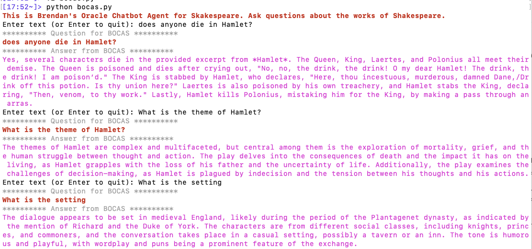
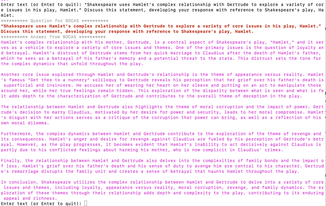
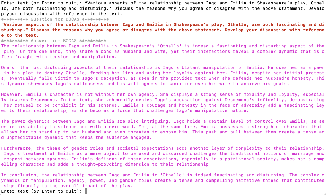
print(Fore.MAGENTA + chat_response.data.message.content.text + Style.RESET_ALL)
print("*** The End - Exiting BOCAS ***")When the above code is run, it will loop, asking for questions, until no question is added and the ‘Enter’ key is pressed. Here is the output of the BOCAS running for some of the questions I asked in my previous post, along with a few others. These questions are based on the Irish Leaving Certificate English Examination.
OCI Gen AI – How to call using Python
Oracle OCI has some Generative AI features, one of which is a Playground allowing you to play or experiment with using several of the Cohere models. The Playground includes Chat, Generation, Summarization and Embedding.
OCI Generative AI services are only available in a few Cloud Regions. You can check the available regions in the documentation. A simple way to check if it is available in your cloud account is to go to the menu and see if it is listed in the Analytics & AI section.

When the webpage opens you can select the Playground from the main page or select one of the options from the menu on the right-hand-side of the page. The following image shows this menu and in this image, I’ve selected the Chat option.

You can enter your questions into the chat box at the bottom of the screen. In the image, I’ve used the following text to generate a Retirement email.
A university professor has decided to retire early. write and email to faculty management and HR of his decision. The job has become very stressful and without proper supports I cannot continue in the role. write me an email for this
Using this playground is useful for trying things out and to see what works and doesn’t work for you. When you are ready to use or deploy such a Generative AI solution, you’ll need to do so using some other coding environment. If you look toward the top right hand corner of this playground page, you’ll see a ‘View code’ button. When you click on this Code will be generated for you in Java and Python. You can copy and paste this to any environment and quickly have a Chatbot up and running in few minutes. I was going to say a few second but you do need to setup a .config file to setup a secure connection to your OCI account. Here is a blog post I wrote about setting this up.
Here is a copy of that Python code with some minor edits, 1) to remove my Compartment ID, 2) I’ve added some message requests. You can comment/uncomment as you like or add something new.
import oci

# Setup basic variables
# Auth Config
# TODO: Please update config profile name and use the compartmentId that has policies grant permissions for using Generative AI Service
compartment_id =  <add your Compartment ID>
CONFIG_PROFILE = "DEFAULT"
config = oci.config.from_file('~/.oci/config', CONFIG_PROFILE)

# Service endpoint
endpoint = "https://inference.generativeai.us-chicago-1.oci.oraclecloud.com"

generative_ai_inference_client = oci.generative_ai_inference.GenerativeAiInferenceClient(config=config, service_endpoint=endpoint, retry_strategy=oci.retry.NoneRetryStrategy(), timeout=(10,240))
chat_detail = oci.generative_ai_inference.models.ChatDetails()

chat_request = oci.generative_ai_inference.models.CohereChatRequest()
#chat_request.message = "Tell me what you can do?"
#chat_request.message = "How does GenAI work?"
chat_request.message = "What's the weather like today where I live?"
chat_request.message = "Could you look it up for me?"
chat_request.message = "Will Elon Musk buy OpenAI?"
chat_request.message = "Tell me about Stargate Project and how it will work?"
chat_request.message = "What is the most recent date your model is built on?"


chat_request.max_tokens = 600
chat_request.temperature = 1
chat_request.frequency_penalty = 0
chat_request.top_p = 0.75
chat_request.top_k = 0
chat_request.seed = None


chat_detail.serving_mode = oci.generative_ai_inference.models.OnDemandServingMode(model_id="ocid1.generativeaimodel.oc1.us-chicago-1.amaaaaaask7dceyanrlpnq5ybfu5hnzarg7jomak3q6kyhkzjsl4qj24fyoq")
chat_detail.chat_request = chat_request
chat_detail.compartment_id = compartment_id
chat_response = generative_ai_inference_client.chat(chat_detail)
# Print result
print("**************************Chat Result**************************")
print(vars(chat_response))
When I run the above code I get the following output.
NB: If you have the OCI Python package already installed you might need to update it to the most recent version
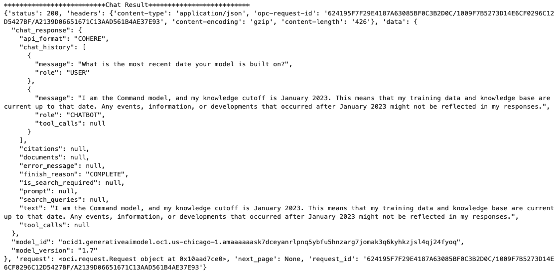
You can see there is a lot generated and returned in the response. We can tidy this up a little using the following and only display the response message.
import json
# Convert JSON output to a dictionary
data = chat_response.__dict__["data"]
output = json.loads(str(data))

# Print the output
print("---Message Returned by LLM---")
print(output["chat_response"]["chat_history"][1]["message"])
That’s it. Give it a try and see how you can build it into your applications.
Using a Gen AI Agent to answer Leaving Certificate English papers
In a previous post, I walked through the steps needed to create a Gen AI Agent on a data set of documents containing the works of Shakespeare. In this post, I’ll look at how this Gen AI Agent can be used to answer questions from the Irish Leaving Certificate Higher Level English examination papers from the past few years.
For this evaluation, I will start with some basic questions before moving on to questions from the Higher Level English examination from 2022, 2023 and 2024. I’ve pasted the output generated below from chatting with the AI Agent.
The main texts we will examine will be Othello, McBeth and Hamlett. Let’s start with some basic questions about Hamlet.
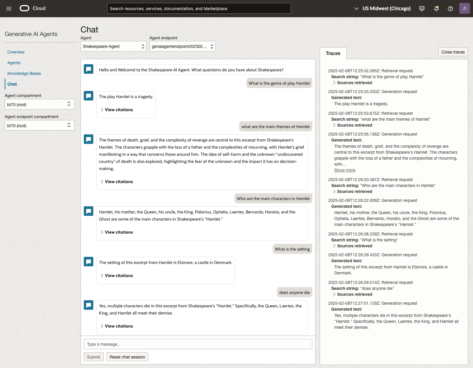
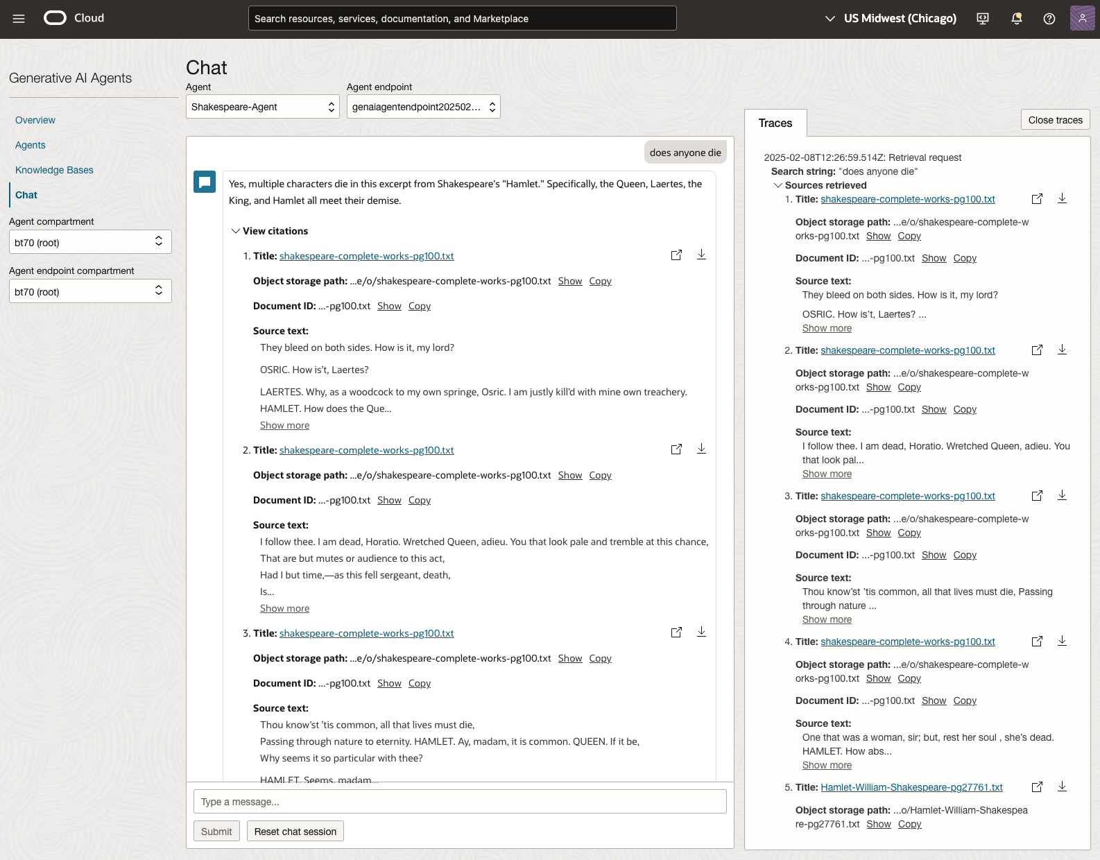
We can look at the sources used by the AI Agent to generate their answer, by clicking on View citations or Sources retrieved on the right-hand side panel.
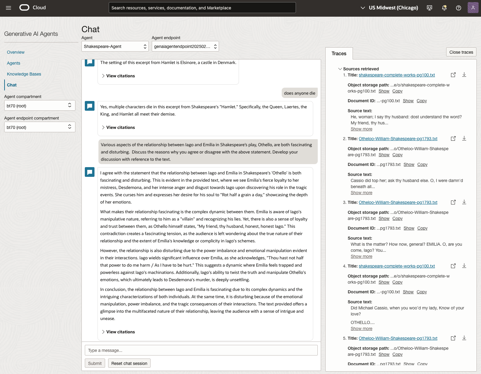
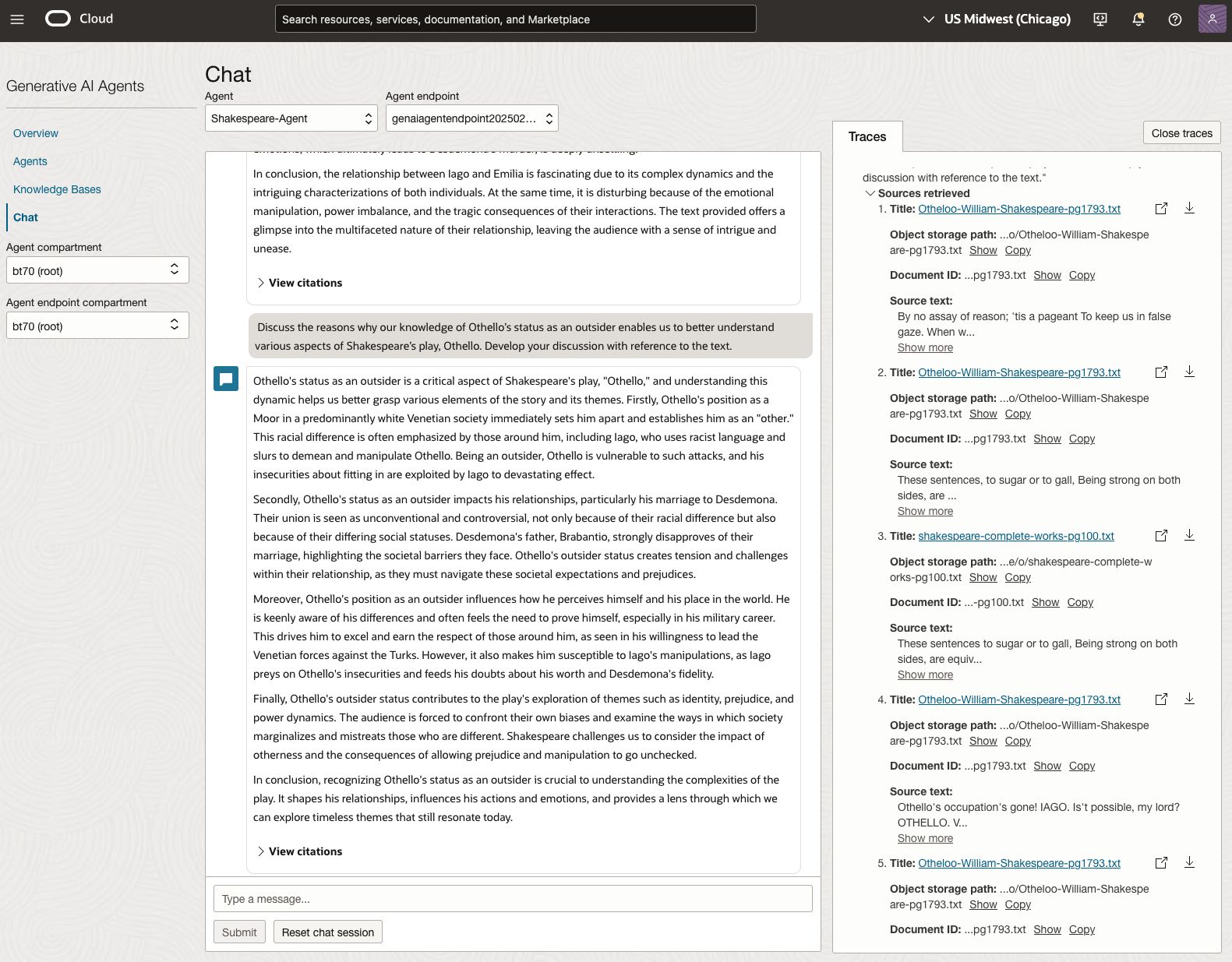
Let’s have a look at the 2022 English examination question on Othello. Students typically have the option of answering one out of two questions.
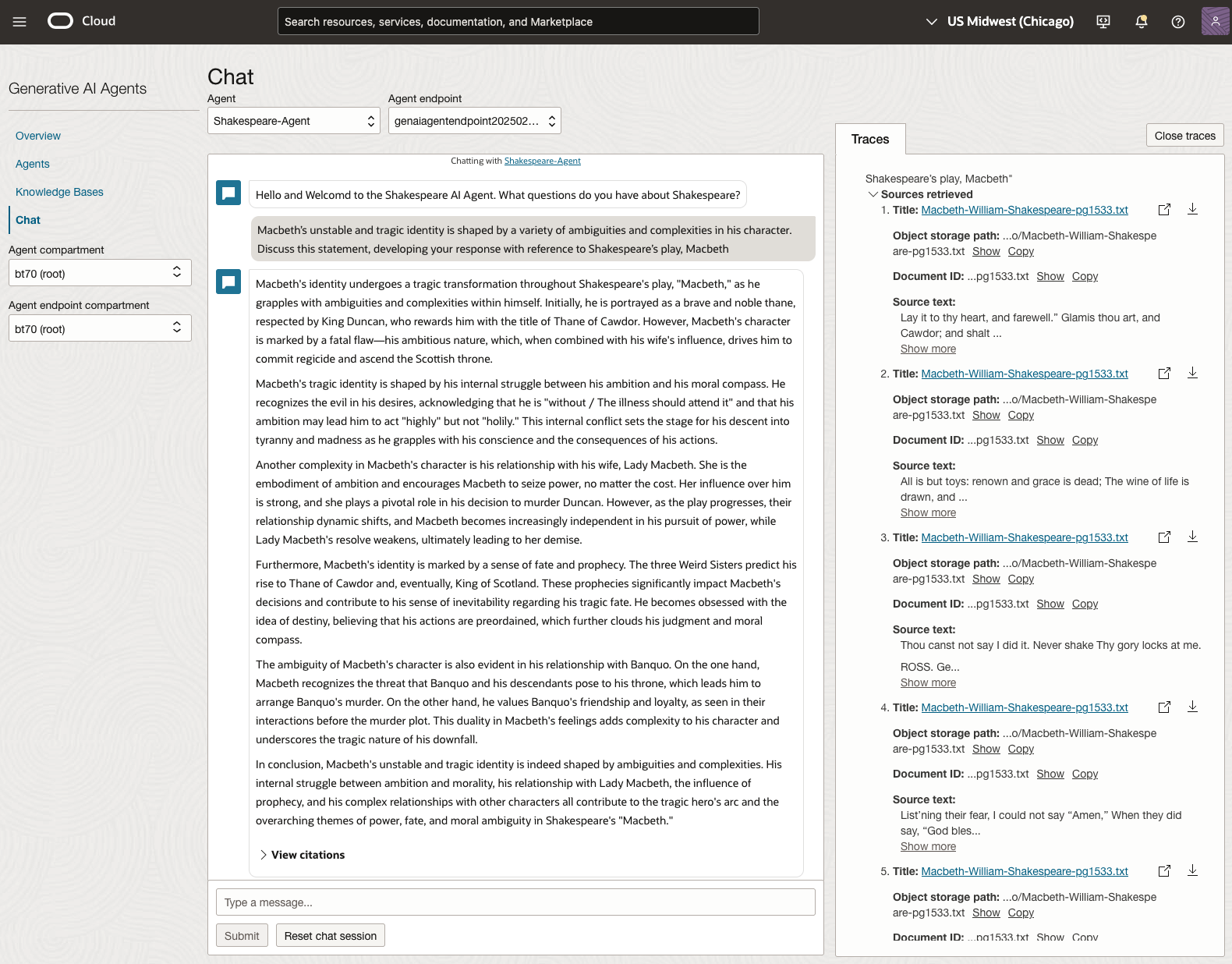
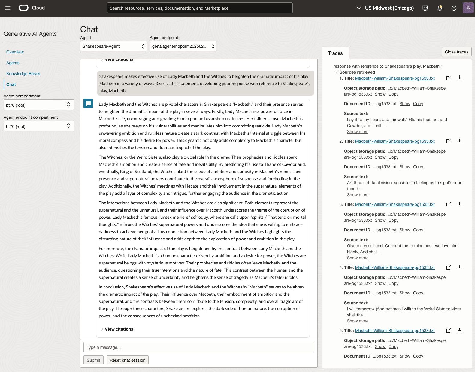
In 2023, the Shakespeare text was McBeth.
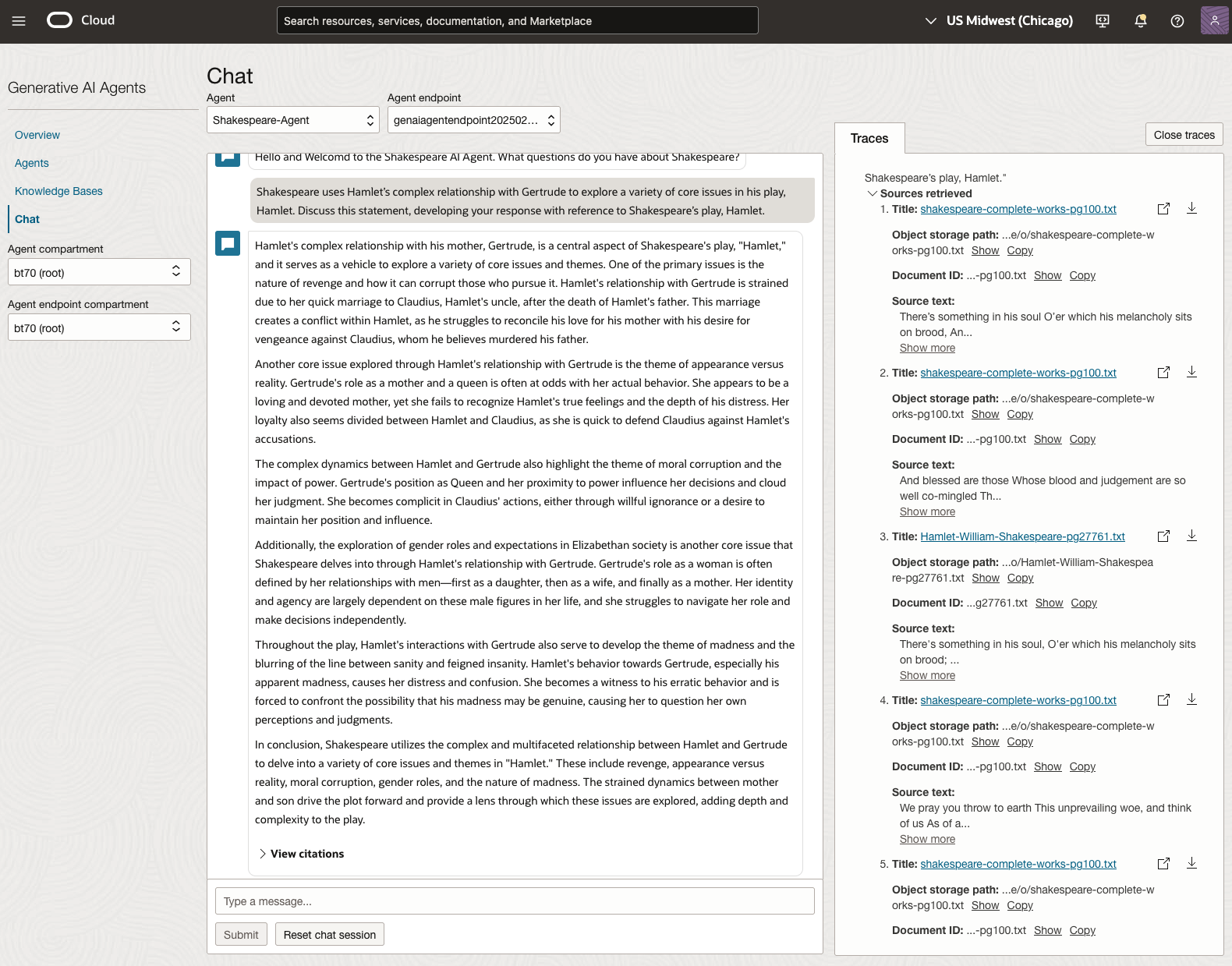
In 2024, the Shakespeare text was Hamlet.
We can see from the above questions, that the AI Agent was able to generate possible answers. As a learning and study resource, it can be difficult to determine the correctness of these answers. Currently, there does seem to be evidence that students typically believe what the AI is generating. But the real question is, should they? Why the AI Agent can give a believable answer for students to memorise, but how good are the answers really? How many marks would they get for these answers? What kind of details are missing from these answers?
To help me answer these questions I enlisted the help of some previous Students who took these English examinations, along with two English teachers who teach higher-level English classes. The students all achieved a H1 grade for English. This is the highest grade possible, where a H1 means they achieved between 90-100%. The feedback from the students and teachers was largely positive. One teacher remarked the answers, to some of the questions, were surprisingly good. When asked about what grade or what percentage range these answers would achieve, again the students and teachers were largely in agreement, with a range between 60-75%. The students tended to give slightly higher marks than the teachers. They were then asked about what was missing from these answers, as in what was needed to get more marks. Again the responses from both the students and teachers were similar, with details of higher-level reasoning, understanding of interpersonal themes, irony, imagery, symbolism, etc were missing.
How to Create an Oracle Gen AI Agent
In this post, I’ll walk you through the steps needed to create a Gen AI Agent on Oracle Cloud. We have seen lots of solutions offered by my different providers for Gen AI Agents. This post focuses on just what is available on Oracle Cloud. You can create a Gen AI Agent manually. However, testing and fine-tuning based on various chunking strategies can take some time. With the automated options available on Oracle Cloud, you don’t have to worry about chunking. It handles all the steps automatically for you. This means you need to be careful when using it. Allocate some time for testing to ensure it meets your requirements. The steps below point out some checkboxes. You need to check them to ensure you generate a more complete knowledge base and outcome.
For my example scenario, I’m going to build a Gen AI Agent for some of the works by Shakespeare. I got the text of several plays from the Gutenberg Project website. The process for creating the Gen AI Agent is:

Step-1 Load Files to a Bucket on OCI
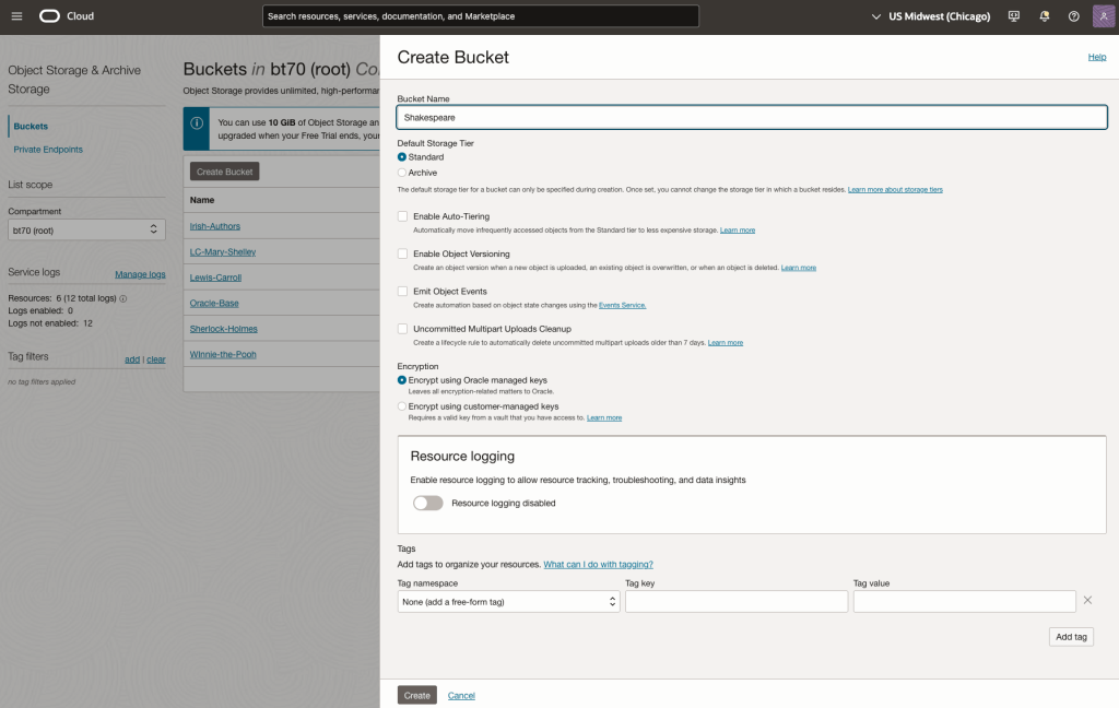
Create a bucket called Shakespeare.
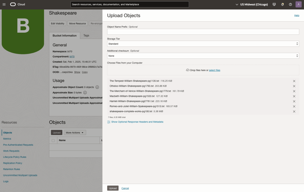
Load the files from your computer into the Bucket. These files were obtained from the Gutenberg Project site.
Step-2 Define a Data Source (documents you want to use) & Create a Knowledge Base
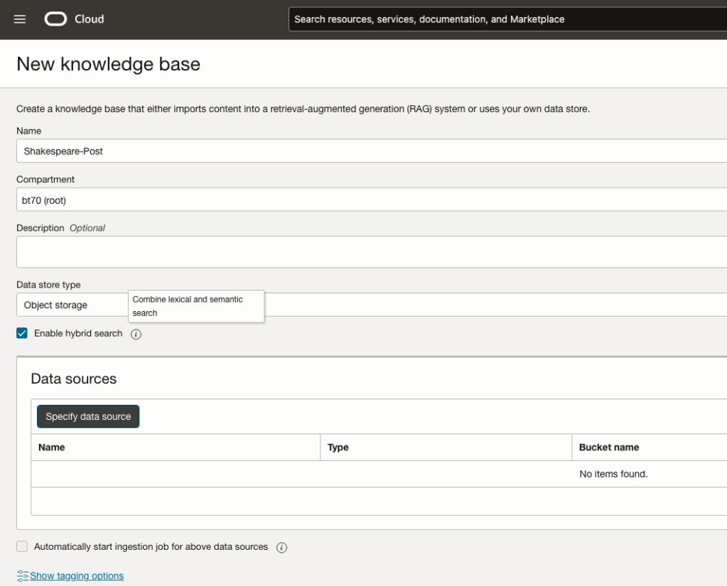
Click on Create Knowledge Base and give it a name ‘Shakespeare’.
Check the ‘Enable Hybrid Search’. checkbox. This will enable both lexical and semantic search. [this is Important]
Click on ‘Specify Data Source’
Select the Bucket from the drop-down list (Shakespeare bucket).
Check the ‘Enable multi-modal parsing’ checkbox.
Select the files to use or check the ‘Select all in bucket’
Click Create.

The Knowledge Base will be created. The files in the bucket will be parsed, and structured for search by the AI Agent. This step can take a few minutes as it needs to process all the files. This depends on the number of files to process, their format and the size of the contents in each file.
Step-3 Create Agent
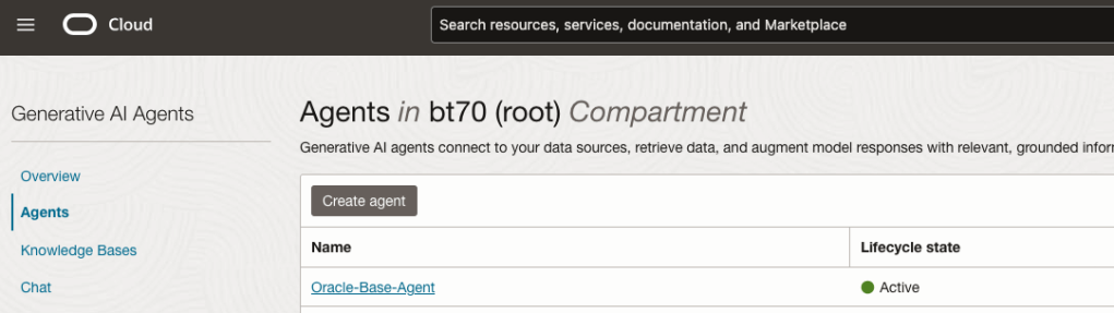
Go back to the main Gen AI menu and select Agent and then Create Agent.
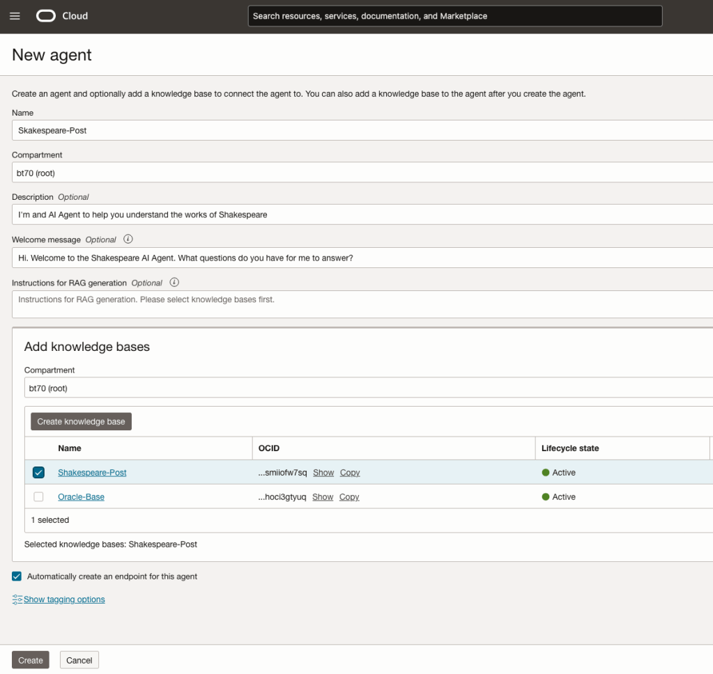
You can enter the following details:
- Name of the Agent
- Some descriptive information
- A Welcome message for people using the Agent
- Select the Knowledge Base from the list.
The checkbox for creating Endpoints should be checked.
Click Create.
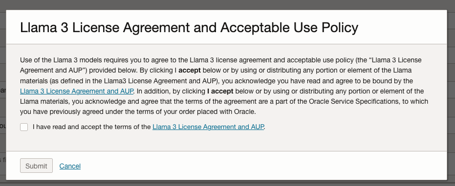
A pop-up window will appear asking you to agree to the Llama 3 License. Check this checkbox and click Submit.
After the agent has been created, check the status of the endpoints. These generally take a little longer to create, and you need these before you can test the Agent using the Chatbot.
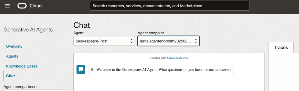
Step-4 Test using Chatbot
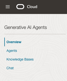
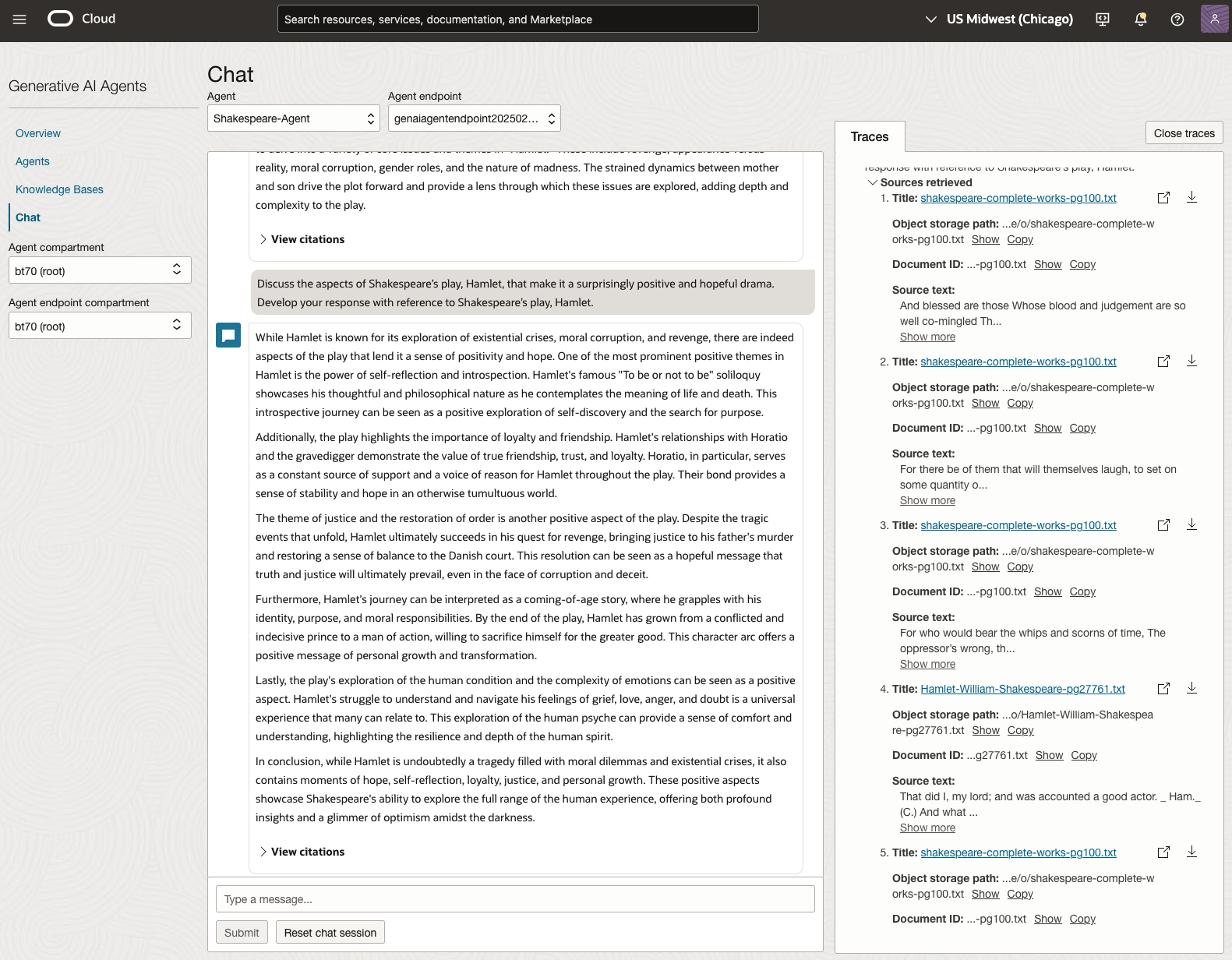
After verifying the endpoints have been created, you can open a Chatbot by clicking on ‘Chat’ from the menu on the left-hand side of the screen.
Select the name of the ‘Agent’ from the drop-down list e.g. Shakespeare-Post.
Select an end-point for the Agent.
After these have been selected you will see the ‘Welcome’ message. This was defined when creating the Agent.
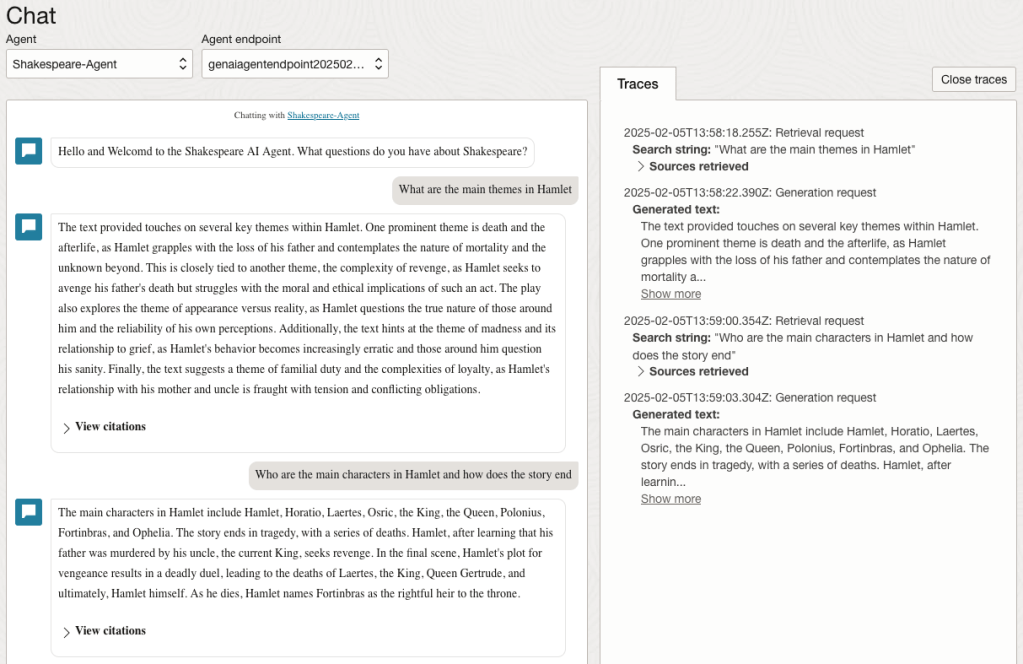
Here are a couple of examples of querying the works by Shakespeare.
In addition to giving a response to the questions, the Chatbot also lists the sections of the underlying documents and passages from those documents used to form the response/answer.
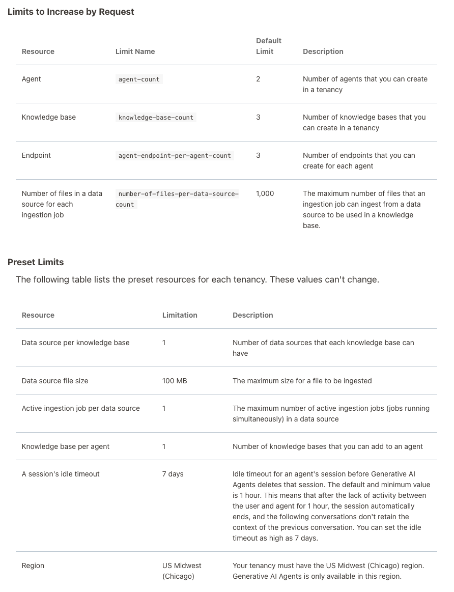
When creating Gen AI Agents, you need to be careful of two things. The first is the Cloud Region. Gen AI Agents are only available in certain Cloud Regions. If they aren’t available in your Region, you’ll need to request access to one of those or setup a new OCI account based in one of those regions. The second thing is the Resource Limits. At the time of writing this post, the following was allowed. Check out the documentation for more details. You might need to request that these limits be increased.
I’ll have another post showing how you can run the Chatbot on your computer or VM as a webpage.
Tracking AI Regulations, Governance and Incidents
Here are the key Trackers to follow to stay ahead.
𝐀𝐈 Incidents & Risks
AI Risk Repository [MIT FutureTech]
A comprehensive database of 700 risks from AI systems https://airisk.mit.edu/
AI Incident Database [Partnership on AI]
Dedicated to indexing the collective history real-world of harms caused by the deployment of AI
https://lnkd.in/ewBaYitm
AI Incidents Monitor [OECD – OCDE]
AI incidents and hazards reported in international media globally are identified and classified using machine learning models https://lnkd.in/e4pJ7jcA
𝐀𝐈 Regulations & Policies
Global AI Law and Policy Tracker [IAPP]
Resource providing information about AI law and policy developments in key jurisdictions worldwide https://lnkd.in/eiGMk9Rm
National AI Policies and Strategies [OECD.AI]
Live repository of 1000+ AI policy initiatives from 69 countries, territories and the EU https://lnkd.in/ebVTQzdb
Global AI Regulation Tracker [Raymond Sun]
An interactive world map that tracks AI law, regulatory and policy developments around the world https://lnkd.in/ekaKzmzD
U.S. State AI Governance Legislation Tracker [IAPP]
Tracker which focuses on cross-sectoral AI governance bills that apply to the private sector https://lnkd.in/ee4N-ckB.
𝐀𝐈 Governance Toolkits & Resources
AI Standards Hub [The Alan Turing Institute]
Online repository of 300+ AI standards https://lnkd.in/erVdP4g7
AI Risk Management Framework Playbook [National Institute of Standards and Technology (NIST)]
Playbook of recommended actions, resources and materials to support implementation of the NIST AI RMF https://lnkd.in/eTzpfbCi
Catalogue of Tools & Metrics for Trustworthy AI [OECD.AI]
Tools and metrics which help AI actors to build and deploy trustworthy AI systems https://lnkd.in/e_mnAbpZ
Portfolio of AI Assurance Techniques [Department for Science, Innovation and Technology]
The Portfolio showcases examples of AI assurance techniques being used in the real-world to support the development of trustworthy AI. https://lnkd.in/eJ5V3uzb
Vector Databases – Part 4 – Vector Indexes
In this post on Vector Databases, I’ll explore some of the commonly used indexing techniques available in Databases. I’ll also explore the Vector Indexes available in Oracle 23c. Be sure to check that section towards the end of the post, where I’ll also include links to other articles in this series.
As with most data in a Databases, indexes are used for fast access to data. They create an organised structure (typically B+ tree) for storing the location of certain values within a table. When searching for data, if an index exists on that data, the index will be used for matching and the location of the records is used to quickly retrieve the data.
Similarly, for Vector searches, we need some way to search through thousands or millions of vectors to find those that best match our search criteria (vector search). For vector search, there are many more calculations to perform. We want to avoid a MxN search space.

Given the nature of Vectors and the the type of search performed on these, databases need to have different types of indexes. Common Vector Index types include Hash-base, Tree-based, Graph-base and Inverted-file. Let’s have a look at each of these.

Hash-based Vector Indexes
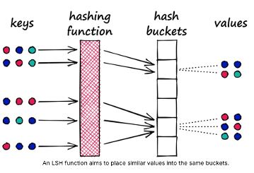
Locality-Sensitive Hashing (LSH) uses hash functions to bucket similar vectors into a hash table. The query vectors are also hashed using the same hash function and it is compared with the other vectors already present in the table. This method is much faster than doing an exhaustive search across the entire dataset because there are fewer vectors in each hash table than in the whole vector space. While this technique is quite fast, the downside is that it is not very accurate. LSH is an approximate method, so a better hash function will result in a better approximation, but the result will not be the exact answer.
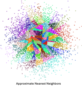
Tree-based Vector Indexes
Tree-based indexing allows for fast searches by using a data structure such as a binary tree. The tree gets created in a way that similar vectors are grouped in the same subtree. Approximate Nearest Neighbour (ANN) uses a forest of binary trees to perform approximate nearest neighbors search. ANN performs well with high-dimension data where doing an exact nearest neighbors search can be expensive. The downside of using this method is that it can take a significant amount of time to build the index. Whenever a new data point is received, the indices cannot be restructured on the fly. The entire index has to be rebuilt from scratch.
Graph-based Vector Indexes
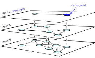
Similar to tree-based indexing, graph-based indexing groups similar data points by connecting them with an edge. Graph-based indexing is useful when trying to search for vectors in a high-dimensional space. Hierarchical Navigable Small Worlds (HNSW) creates a layered graph with the topmost layer containing the fewest points and the bottom layer containing the most points. When an input query comes in, the topmost layer is searched via ANN. The graph is traversed downward layer by layer. At each layer, the ANN algorithm is run to find the closest point to the input query. Once the bottom layer is hit, the nearest point to the input query is returned. Graph-based indexing is very efficient because it allows one to search through a high-dimensional space by narrowing down the location at each layer. However, re-indexing can be challenging because the entire graph may need to be recreated
Inverted-FIle Vector Indexes
IVF (InVerted File) narrows the search space by partitioning the dataset and creating a centroid(random point) for each partition. The centroids get updated via the K-Means algorithm. Once the index is populated, the ANN algorithm finds the nearest centroid to the input query and only searches through that partition. Although IVF is efficient at searching for similar points once the index is created, the process of creating the partitions and centroids can be quite slow.

Oracle 23ai comes with two main types of indexes for Vectors. These are:
In-Memory – Neighbor Graph Vector Index
Hierarchical Navigable Small World (HNSW) is the only type of In-Memory Neighbor Graph vector index supported. With Navigable Small World (NSW), the idea is to build a proximity graph where each vector in the graph connects to several others based on three characteristics:
- The distance between vectors
- The maximum number of closest vector candidates considered at each step of the search during insertion (EFCONSTRUCTION)
- Within the maximum number of connections (NEIGHBORS) permitted per vector
Navigable Small World (NSW) graph traversal for vector search begins with a predefined entry point in the graph, accessing a cluster of closely related vectors. The search algorithm employs two key lists:
- Candidates, a dynamically updated list of vectors that we encounter while traversing the graph,
- and Results, which contains the vectors closest to the query vector found thus far.
As the search progresses, the algorithm navigates through the graph, continually refining the Candidates by exploring and evaluating vectors that might be closer than those in the Results. The process concludes once there are no vectors in the Candidates closer than the farthest in the Results, indicating

Neighbor Partition Vector Index
Inverted File Flat (IVF) index is the only type of Neighbor Partition vector index supported.
Inverted File Flat Index (IVF Flat or simply IVF) is a partitioned-based index which balance high search quality with reasonable speed.
The IVF index is a technique designed to enhance search efficiency by narrowing the search area through the use of neighbor partitions or clusters.

Here is an example of creating such an index in Oracle 23ai.
CREATE VECTOR INDEX galaxies_ivf_idx ON galaxies (embedding)
ORGANIZATION NEIGHBOR
PARTITIONS DISTANCE COSINE
WITH TARGET ACCURACY 95;
Check out my other posts in this series on Vector Databases.

You must be logged in to post a comment.