
SQL Server
Annual Look at Database Trends (Jan 2023)
Monitoring trends in the popularity and usage of different Database vendors can be a interesting exercise. The marketing teams from each vendor do an excellent job of promoting their Database, along with the sales teams, developer advocates, and the user communities. Some of these are more active than others and it varies across the Database market on what their choice is for promoting their products. One of the problems with these various types of marketing, is how can be believe what they are saying about how “awesome” their Database is, and then there are some who actively talk about how “rubbish” (or saying something similar) other Databases area. I do wonder how this really works for these people and vendors when to go negative about their competitors. A few months ago I wrote about “What does Legacy Really Mean?“. That post was prompted by someone from one Database Vendor calling their main competitor Database a legacy product. They are just name calling withing providing any proof or evidence to support what they are saying.
Getting back to the topic of this post, I’ve gathered some data and obtained some league tables from some sites. These will help to have a closer look at what is really happening in the Database market throughout 2022. Two popular sites who constantly monitor the wider internet and judge how popular Databases area globally. These sites are DB-Engines and TOPDB Top Database index. These are well know and are frequently cited. Both of these sites give some details of how they calculate their scores, with one focused mainly on how common the Database appears in searches across different search engines, while the other one, in addition to search engine results/searches, also looks across different websites, discussion forms, social media, job vacancies, etc.
The first image below is a comparison of the league tables from DB-Engines taken in January 2022 and January 2023. I’ve divided this image into three sections/boxes. Overall for the first 10 places, not a lot has changed. The ranking scores have moved slightly in most cases but not enough to change their position in the rank. Even with a change of score by 30+ points is a very small change and doesn’t really indicate any great change in the score as these scores are ranked in a manner where, “when system A has twice as large a value in the DB-Engines Ranking as system B, then it is twice as popular when averaged over the individual evaluation criteria“. Using this explanation, Oracle would be twice as popular when compared to PostgreSQL. This is similar across 2022 and 2023.

Next we’ll look a ranking from TOPDB Top Database index. The image below compares January 2022 and January 2023. TOPDB uses a different search space and calculation for its calculation. The rankings from TOPDB do show some changes in the ranks and these are different to those from DB-Engines. Here we see the top three ranks remain the same with some small percentage changes, and nothing to get excited about. In the second box covering ranks 4-7 we do some changes with PostgreSQL improving by two position and MongoDB. These changes do seem to reflect what I’ve been seeing in the marketplace with MongoDB being replaced by PostgreSQL and MySQL, with this multi-model architecture where you can have relational, document, and other data models in the one Database. It’s important to note Oracle and SQL Server also support this. Over the past couple of years there has been a growing awareness of and benefits of having relation and document (and others) data models in the one database. This approach makes sense both for developer productivity, and for data storage and management.

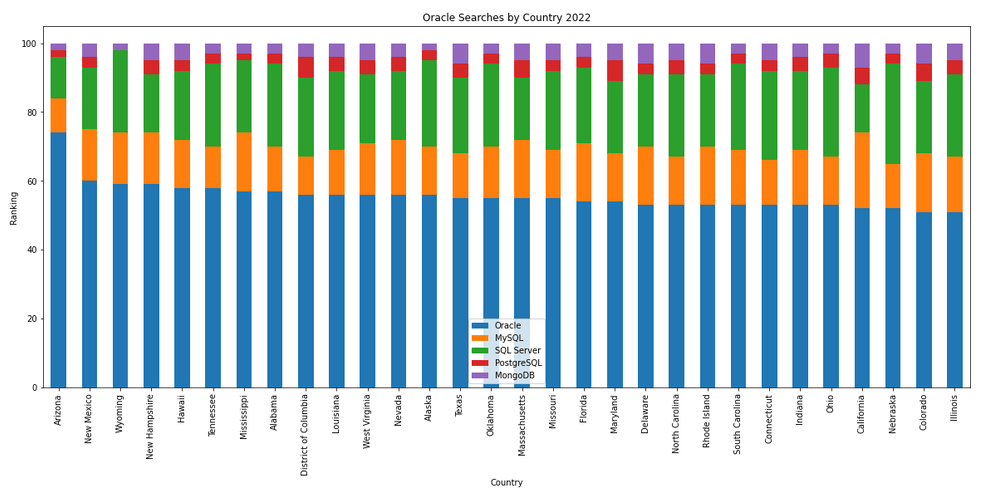
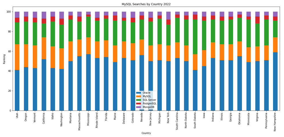
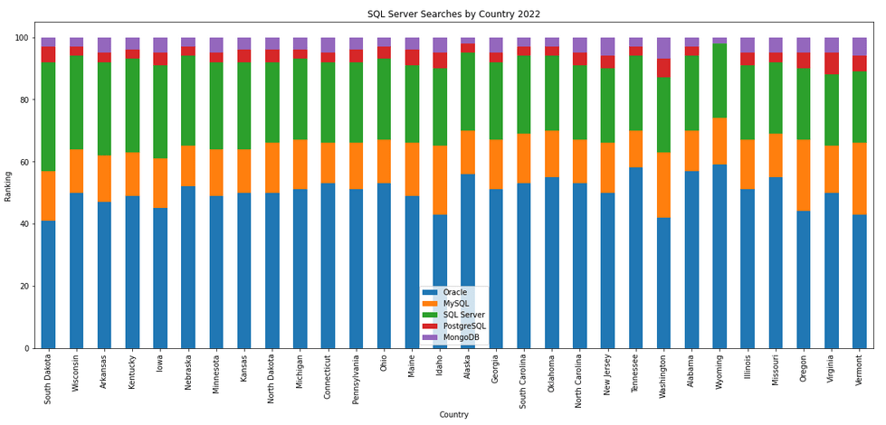
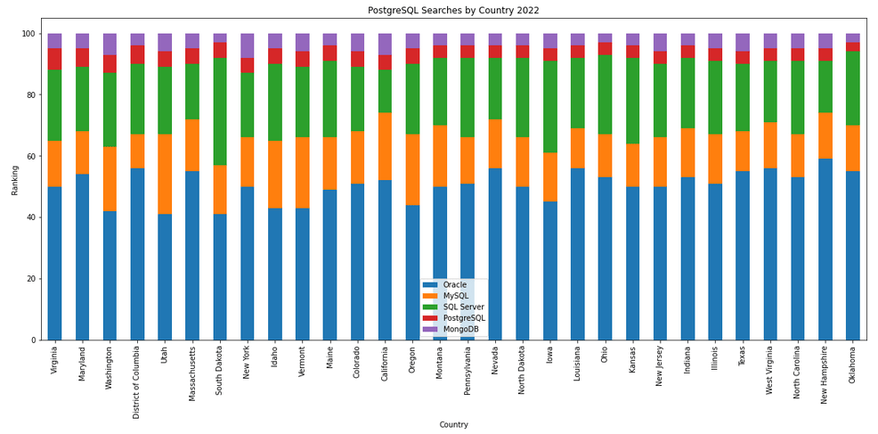
The next gallery of images is based on some Python code I’ve written to look a little bit closer at the top five Databases. In this case these are Oracle, MySQL, SQL Server, PostgreSQL and MongoDB. This gallery plots a bar chart for each Database for their top 15 Counties, and compares them with the other four Databases. The results are interesting and we can see some geographic aspects to the popularity of the Databases.
Number of rows in each Table – Various Databases
A possible common task developers perform is to find out how many records exists in every table in a schema. In the examples below I’ll show examples for the current schema of the developer, but these can be expanded easily to include tables in other schemas or for all schemas across a database.
These example include the different ways of determining this information across the main databases including Oracle, MySQL, Postgres, SQL Server and Snowflake.
A little warning before using these queries. They may or may not give the true accurate number of records in the tables. These examples illustrate extracting the number of records from the data dictionaries of the databases. This is dependent on background processes being run to gather this information. These background processes run from time to time, anything from a few minutes to many tens of minutes. So, these results are good indication of the number of records in each table.
Oracle
SELECT table_name, num_rows
FROM user_tables
ORDER BY num_rows DESC;
or
SELECT table_name,
       to_number(
          extractvalue(xmltype(
             dbms_xmlgen.getxml('select count(*) c from '||table_name))
                ,'/ROWSET/ROW/C')) tab_count
FROM   user_tables
ORDER BY tab_count desc;
Using PL/SQL we can do something like the following.
DECLARE
   val NUMBER;
BEGIN
   FOR i IN (SELECT table_name FROM user_tables ORDER BY table_name desc) LOOP
      EXECUTE IMMEDIATE 'SELECT count(*) FROM '|| i.table_name INTO val;
      DBMS_OUTPUT.PUT_LINE(i.table_name||' -> '|| val );
   END LOOP;
END;
MySQL
SELECT table_name, table_rows
FROM INFORMATION_SCHEMA.TABLES
WHERE table_type = 'BASE TABLE'
AND  TABLE_SCHEMA = current_user();
Using Common Table Expressions (CTE), using WITH clause
WITH table_list AS (
SELECT
    table_name
  FROM information_schema.tables
  WHERE table_schema = current_user()
  AND
        table_type = 'BASE TABLE'
)
SELECT CONCAT(
            GROUP_CONCAT(CONCAT("SELECT '",table_name,"' table_name,COUNT(*) rows FROM ",table_name) SEPARATOR " UNION "),
            ' ORDER BY table_name'
        )
INTO @sql
FROM table_list;
Postgres
select relname as table_name, n_live_tup as num_rows from pg_stat_user_tables;
An alternative is
select n.nspname as table_schema,
       c.relname as table_name,
       c.reltuples as rows
from pg_class c
join pg_namespace n on n.oid = c.relnamespace
where c.relkind = 'r'
      and n.nspname = current_user
order by c.reltuples desc;
SQL Server
SELECT tab.name,
       sum(par.rows)
FROM   sys.tables tab INNER JOIN sys.partitions par
          ON tab.object_id = par.object_id
WHERE  schema_name(tab.schema_id) = current_user
Snowflake
SELECT t.table_schema, t.table_name, t.row_count
FROM   information_schema.tables t
WHERE  t.table_type = 'BASE TABLE'
AND    t.table_schema = current_user
order by t.row_count desc;
The examples give above are some of the ways to obtain this information. As with most things, there can be multiple ways of doing it, and most people will have their preferred one which is based on their background and preferences.
As you can see from the code given above they are all very similar, with similar syntax, etc. The only thing different is the name of the data dictionary table/view containing the information needed. Yes, knowing what data dictionary views to query can be a little challenging as you switch between databases.
Using SQL to create some festive Christmas Trees
Here are a few examples I found on the “great internet” of how SQL can be used to create some festive Christmas cheer and fun. See links to the original posts. Most of the examples shown below have been run on Oracle 21c Docker image, or on SQL Server or MySQL.
Our first example comes from Gerald Venzi who posted this on twitter. See later in the post for Christmas trees created using similar SQL queries.
WITH tree(lev, xmas) AS (
   SELECT 1 lev, RPAD(' ', 10, ' ') || '*' xmas
   FROM dual
   UNION ALL
   SELECT tree.lev+1,
          RPAD(' ', 10-tree.lev, ' ') ||
             RPAD('^', tree.lev+1, '^') ||
             LPAD('^', tree.lev, '^')  xmas
   FROM tree
   WHERE tree.lev < 10
)
SELECT '    Merry Christmas!' AS "Merry Christmas!" FROM dual
UNION ALL
SELECT xmas FROM TREE
UNION ALL
SELECT '         | |' FROM dual
UNION ALL
SELECT '      ~~/   \~~' FROM dual;
Our next example includes using Spatial Data on SQL Server to create a Christmas Tree. This example comes from Niket Kedia.
USE tempdb
GO

— Create a table

CREATE TABLE #xmasTREE (shape GEOMETRY )

–Creating the Christmas tree with stars

INSERT INTO #xmasTREE

VALUES
(‘POLYGON((4 0, 0 0, 4 2, 1 2, 4 4, 1 4, 4 6, 2 6, 5 10, 8 6, 6 6, 9 4, 6 4, 9 2, 6 2, 10 0, 4 0))’ ),
(‘POLYGON((3.5 0, 4 -1, 6 -1, 6.5 0, 3.5 0))’ ),
(‘POLYGON((5 9.5, 4.5 9.25, 4.6 9.9, 4.1 10.2, 4.8 10.2, 5 10.9, 5.2 10.2, 5.9 10.2, 5.4 9.9, 5.5 9.25, 5 9.5))’ ),
(‘POLYGON((2 5.5, 1.5 5.25, 1.6 5.9, 1.1 6.2, 1.8 6.2, 2 6.9, 2.2 6.2, 2.9 6.2, 2.4 5.9, 2.5 5.25, 2 5.5))’ ),
(‘POLYGON((8 5.5, 7.5 5.25, 7.6 5.9, 7.1 6.2, 7.8 6.2, 8 6.9, 8.2 6.2, 8.9 6.2, 8.4 5.9, 8.5 5.25, 8 5.5))’ ),
(‘POLYGON((1 3.5, 0.5 3.25, 0.6 3.9, 0.1 4.2, 0.8 4.2, 1 4.9, 1.2 4.2, 1.9 4.2, 1.4 3.9, 1.5 3.25, 1 3.5))’ ),
(‘POLYGON((9 3.5, 8.5 3.25, 8.6 3.9, 8.1 4.2, 8.8 4.2, 9 4.9, 9.2 4.2, 9.9 4.2, 9.4 3.9, 9.5 3.25, 9 3.5))’ ), (‘POLYGON((1 1.5, 0.5 1.25, 0.6 1.9, 0.1 2.2, 0.8 2.2, 1 2.9, 1.2 2.2, 1.9 2.2, 1.4 1.9, 1.5 1.25, 1 1.5))’ ), (‘POLYGON((9 1.5, 8.5 1.25, 8.6 1.9, 8.1 2.2, 8.8 2.2, 9 2.9, 9.2 2.2, 9.9 2.2, 9.4 1.9, 9.5 1.25, 9 1.5))’ ),
(‘POLYGON((0 -0.5, -0.5 -0.75, -0.4 -0.1, -0.9 0.2, -0.2 0.2, 0 0.9, 0.2 0.2, 0.9 0.2, 0.4 -0.1, 0.5 -0.75, 0 -0.5))’ ),
(‘POLYGON((10 -0.5, 9.5 -0.75, 9.6 -0.1, 9.1 0.2, 9.8 0.2, 10 0.9, 10.2 0.2, 10.9 0.2, 10.4 -0.1, 10.5 -0.75, 10 -0.5))’ ),
(‘POLYGON((5 -2, 4.5 -2, 4.5 -1, 5 -1, 5.5 -1, 5.5 -2, 5 -2))’)

–Create the “Merry Christmas” greetings

INSERT INTO #xmasTREE

VALUES (‘POLYGON((-2 11, -2 12, -1.75 12, -1.5 11.5, -1.25 12, -1 12, -1 11, -1.25 11, -1.25 11.7, -1.5 11.2, -1.75 11.7, -1.75 11, -2 11))’ ),–M
(‘POLYGON((-1 11, -1 12, 0 12, 0 11.8, -0.75 11.8, -0.75 11.6, -0.25 11.6, -0.25 11.4, -0.75 11.4, -0.75 11.2, 0 11.2, 0 11, -1 11))’ ),–E
(‘POLYGON((0 11, 0 12, 1 12, 1 11.5, 0.4 11.5, 1 11, 0.7 11, 0.2 11.4, 0.2 11, 0 11),(0.2 11.8, 0.8 11.8, 0.8 11.7, 0.2 11.7, 0.2 11.8))’ ),–R
(‘POLYGON((1 11, 1 12, 2 12, 2 11.5, 1.4 11.5, 2 11, 1.7 11, 1.2 11.4, 1.2 11, 1 11),(1.2 11.8, 1.8 11.8, 1.8 11.7, 1.2 11.7, 1.2 11.8))’ ),–R
(‘POLYGON((2 12, 2.2 12, 2.5 11.6, 2.8 12, 3 12, 2.6 11.5, 2.6 11, 2.4 11, 2.4 11.5, 2 12))’ ), –Y
(‘POLYGON((4 11, 4 12, 5 12, 5 11.8, 4.25 11.8, 4.25 11.2, 5 11.2, 5 11, 4 11))’ ),–C
(‘POLYGON((5 11, 5 12, 5.2 12, 5.2 11.6, 5.8 11.6, 5.8 12, 6 12, 6 11, 5.8 11, 5.8 11.4, 5.2 11.4, 5.2 11, 5 11))’ ),–H
(‘POLYGON((6 11, 6 12, 7 12, 7 11.5, 6.4 11.5, 7 11, 6.7 11, 6.2 11.4, 6.2 11, 6 11),(6.2 11.8, 6.8 11.8, 6.8 11.7, 6.2 11.7, 6.2 11.8))’ ),–R
(‘POLYGON((7.2 11, 7.2 11.2, 7.4 11.2, 7.4 11.8, 7.2 11.8, 7.2 12, 7.8 12, 7.8 11.8, 7.6 11.8, 7.6 11.2, 7.8 11.2, 7.8 11, 7.2 11))’ ),–I
(‘POLYGON((8 11, 8 11.2, 8.8 11.2, 8.8 11.4, 8 11.4, 8 12, 9 12, 9 11.8, 8.2 11.8, 8.2 11.6, 9 11.6, 9 11, 8 11))’ ),–S
(‘POLYGON((9 11.8, 9 12, 10 12, 10 11.8, 9.6 11.8, 9.6 11, 9.4 11, 9.4 11.8, 9 11.8))’ ),–T
(‘POLYGON((10 11, 10 12, 10.25 12, 10.5 11.5, 10.75 12, 11 12, 11 11, 10.75 11, 10.75 11.7, 10.5 11.2, 10.25 11.7, 10.25 11, 10 11))’ ),–M
(‘POLYGON((11 11, 11 12, 12 12, 12 11, 11.75 11, 11.75 11.3, 11.25 11.3, 11.25 11, 11 11),(11.25 11.5, 11.25 11.8, 11.75 11.8, 11.75 11.5, 11.25 11.5))’ ),–A
(‘POLYGON((12 11, 12 11.2, 12.8 11.2, 12.8 11.4, 12 11.4, 12 12, 13 12, 13 11.8, 12.2 11.8, 12.2 11.6, 13 11.6, 13 11, 12 11))’ )–S

–Decorate the tree with some round bell circles

DECLARE @counter INT = 0

,@x INT

,@y INT ;

WHILE ( @counter < 25 )

BEGIN

INSERT INTO #xmasTREE

VALUES (GEOMETRY::Point(RAND() * 5 + 2.5, RAND() * 8.5, 0).STBuffer(0.3) )

SET @counter+=1 ;

END

Select * from #xmasTREE
Drop table #xmasTREE
Our next example comes from StackOverflow with a similar example for MySQL.
DECLARE @g TABLE (g GEOMETRY, ID INT IDENTITY(1,1));


-- Adjust Color

INSERT INTO @g(g) SELECT TOP 29 CAST('POLYGON((0 0, 0 0.0000001, 0.0000001 0.0000001, 0 0))' as geometry) FROM sys.messages;

-- Build Christmas Tree

INSERT INTO @g(g) VALUES (CAST('POLYGON((0 0,900 0,450 400, 0 0 ))' as geometry).STUnion(CAST('POLYGON((80 330,820 330,450 640,80 330 ))' as geometry)).STUnion(CAST('POLYGON((210 590,690 590,450 800, 210 590 ))' as geometry)));

-- Adjust Color

INSERT INTO @g(g) SELECT TOP 294 CAST('POLYGON((0 0, 0 0.0000001, 0.0000001 0.0000001, 0 0))' as geometry) FROM sys.messages;

-- Build a Star

INSERT INTO @g(g) VALUES (CAST('POLYGON ((450 910, 465.716 861.631, 516.574 861.631, 475.429 831.738, 491.145 783.369, 450 813.262, 408.855 783.369, 424.571 831.738, 383.426 861.631, 434.284 861.631, 450 910))' as geometry));

-- Build Colored Balls

INSERT INTO @g(g) SELECT TOP 2 CAST('POLYGON((0 0, 0 0.0000001, 0.0000001 0.0000001, 0 0))' as geometry) FROM sys.messages;

INSERT INTO @g(g) VALUES (CAST('CURVEPOLYGON (CIRCULARSTRING (80 290, 110 320, 140 290, 110 260, 80 290))' as geometry));

INSERT INTO @g(g) SELECT TOP 2 CAST('POLYGON((0 0, 0 0.0000001, 0.0000001 0.0000001, 0 0))' as geometry) FROM sys.messages;

INSERT INTO @g(g) VALUES (CAST('CURVEPOLYGON (CIRCULARSTRING (760 290, 790 320, 820 290, 790 260, 760 290))' as geometry));

INSERT INTO @g(g) SELECT TOP 3 CAST('POLYGON((0 0, 0 0.0000001, 0.0000001 0.0000001, 0 0))' as geometry) FROM sys.messages;

INSERT INTO @g(g) VALUES (CAST('CURVEPOLYGON (CIRCULARSTRING (210 550, 240 580, 270 550, 240 520, 210 550))' as geometry));

INSERT INTO @g(g) SELECT TOP 46 CAST('POLYGON((0 0, 0 0.0000001, 0.0000001 0.0000001, 0 0))' as geometry) FROM sys.messages;

INSERT INTO @g(g) VALUES (CAST('CURVEPOLYGON (CIRCULARSTRING (630 550, 660 580, 690 550, 660 520, 630 550))' as geometry));


SELECT g FROM @g ORDER BY ID;

GO
Connor McDonold posted the following SQL to create a Christmas Tree on StackOverflow in 2020, and wrote a blog post for it in December 2021. I just made one very very minor change to it.
You need to be careful where you run this. It runs best on/in a Linux environment, docker, VM, etc using SQL Command Line or SQL*Plus. For me, SQL Developer struggled to present the results correctly.
select replace(replace(replace(r,'X',chr(27)||'[42m'||chr(27)||'[1;'||to_char(32)||'m'||'X'||chr(27)||'[0m'),
    'T',chr(27)||'[43m'||chr(27)||'[1;'||to_char(33)||'m'||'T'||chr(27)||'[0m'),
    '@',chr(27)||'[33m'||chr(27)||'[1;'||to_char(31)||'m'||'@'||chr(27)||'[0m')  Happy_Christmas
from ( select lpad(' ',20-e-i)|| case when dbms_random.value < 0.3 then substr(s,1,e*2-3+i*2)
       else substr(substr(s,1,dbms_random.value(1,e*2-3+i*2-1))||'@'||s,1,e*2-3+i*2) end r
from ( select rpad('X',40,'X') s,rpad('T',40,'T') t from dual ) ,
( select level i, level+2 hop from dual connect by level <= 4 ) , lateral
( select level e from dual connect by level <= hop ) union all select lpad(' ',17)||substr(t,1,3)
from ( select rpad('X',40,'X') s,rpad('T',40,'T') t from dual ) connect by level <= 5 );
Next up we have a simpler Christmas Tree. This comes from Matheus Boesing and his original post on grepora.
clear screen
set feedback off;
set heading off;
set pages 80;
SELECT DECODE(SIGN(FLOOR(maxwidth / 2) - ROWNUM),
              1,
              LPAD(' ', FLOOR(maxwidth / 2) - (ROWNUM - 1)) ||
              RPAD('*', 2 * (ROWNUM - 1) + 1, ' *'),
              LPAD('* * *', FLOOR(maxwidth / 2) + 3))
  FROM all_objects, (SELECT 40 AS maxwidth FROM DUAL)
 WHERE ROWNUM < FLOOR(maxwidth / 2) + 5
union all select '     Happy Christmas from Brendan!' from dual;
set heading on;
set feedback on;
This next example comes from LearnSQL and is similar to the previous example, but this time we get a multiple trees.
clear screen
set feedback off;
set heading off;
set pages 80;
WITH small_tree(tree_depth,pine) AS (
  SELECT 1 tree_depth,
  rpad(' ',10,' ') || '*'
  || rpad(' ',20,' ') || '*'
  || rpad(' ',20,' ') || '*'
  pine
  FROM   dual
  UNION ALL
  SELECT small_tree.tree_depth +1 tree_depth,
  rpad(' ',10-small_tree.tree_depth,' ') || rpad('*',small_tree.tree_depth+1,'.') || lpad('*',small_tree.tree_depth,'.')
  || rpad(' ',20-small_tree.tree_depth-tree_depth,' ') || rpad('*',small_tree.tree_depth+1,'.') || lpad('*',small_tree.tree_depth,'.')
  || rpad(' ',20-small_tree.tree_depth-tree_depth,' ') || rpad('*',small_tree.tree_depth+1,'.') || lpad('*',small_tree.tree_depth,'.') pine
  FROM   small_tree
  where small_tree.tree_depth < 10
)
SELECT   rpad(' ',9,' ') ||'Ho'
         || rpad(' ',19,' ') || 'Ho'
         || rpad(' ',19,' ') || 'Ho'
  pine
  FROM   dual
  UNION ALL
SELECT pine
FROM small_tree;
set heading on;
set feedback on;
Hans Viehmann from the Oracle Spatial teams sent me this example using Oracle Spatial and Oracle Spatial Studio. The geospatial data is defined using GeoJSON. The funny coordinates are referencing the Santa Claus village near Rovaniemi in Finnish Lappland, right on the Arctic Circle. Oracle Spatial Studio can be used to view the Christmas tree on a map (see image below).
DROP TABLE XMAS_TREE_JSON;

DROP TABLE XMAS_TREE;

CREATE TABLE XMAS_TREE_JSON (
    ID   NUMBER(10),
    DATA CLOB,
    CONSTRAINT XMAS_TREE_PK PRIMARY KEY ( ID ),
    CONSTRAINT XMAS_TREE_JSON_CHK CHECK ( DATA IS JSON )
);

INSERT INTO XMAS_TREE_JSON VALUES (
    1,
    '{
      "type": "Feature",
      "properties": { "label": "Tree"},
      "geometry": {
        "type": "Polygon",
        "coordinates": [
          [[25.84725335240364,
              66.5437744044363],
            [25.847166180610653,
              66.543721555766],
            [25.847235918045044,
              66.5437231572425],
            [25.84712728857994,
              66.5436740452493],
            [25.84722116589546,
              66.54367564672889],
            [25.847095102071762,
              66.54362012871027],
            [25.847205072641373,
              66.54362226402098],
            [25.847202390432358,
              66.54361105363778],
            [25.847297608852386,
              66.54361212129352],
            [25.847297608852386,
              66.5436238655039],
            [25.84740623831749,
              66.5436243993315],
            [25.84728017449379,
              66.54367724820834],
            [25.84736466407776,
              66.54367724820834],
            [25.847273468971252,
              66.54372369106797],
            [25.847321748733517,
              66.54372369106797],
            [25.84725335240364,
              66.5437744044363]
          ]
        ]
      }
    }'
);

COMMIT;

CREATE TABLE XMAS_TREE
    AS
        SELECT
            ID,
            JSON_VALUE(DATA, '$.geometry' RETURNING SDO_GEOMETRY) AS SHAPE,
            JSON_VALUE(DATA, '$.properties.label')                AS LABEL
        FROM
            XMAS_TREE_JSON;
Happy Christmas everyone.
Exploring Database trends using Python pytrends (Google Trends)
A little word of warning before you read the rest of this post. The examples shown below are just examples of what is possible. It isn’t very scientific or rigorous, so don’t come complaining if what is shown doesn’t match your knowledge and other insights. This is just a little fun to see what is possible. Yes a more rigorous scientific study is needed, and some attempts at this can be seen at DB-Engines.com. Less scientific are examples shown at TOPDB Top Database index and that isn’t meant to be very scientific.
After all of that, here we go 🙂
pytrends is a library providing an API to Google Trends using Python. The following examples show some ways you can use this library and the focus area I’ll be using is Databases. Many of you are already familiar with using Google Trends, and if this isn’t something you have looked at before then I’d encourage you to go have a look at their website and to give it a try. You don’t need to run Python to use it. For example, here is a quick example taken from the Google Trends website. Here are a couple of screen shots from Google Trends, comparing Relational Database to NoSQL Database. The information presented is based on what searches have been performed over the past 12 months. Some of the information is kind of interesting when you look at the related queries and also the distribution of countries.


To install pytrends use the pip command
pip3 install pytrends
As usual it will change the various pendent libraries and will update where necessary. In my particular case, the only library it updated was the version of pandas.
You do need to be careful of how many searches you perform as you may be limited due to Google rate limits. You can get around this by using a proxy and there is an example on the pytrends PyPi website on how to get around this.
The following code illustrates how to import and setup an initial request. The pandas library is also loaded as the data returned by pytrends API into a pandas dataframe. This will make it ease to format and explore the data.
import pandas as pd
from pytrends.request import TrendReq

pytrends = TrendReq()
The pytrends API has about nine methods. For my example I’ll be using the following:
- Interest Over Time: returns historical, indexed data for when the keyword was searched most as shown on Google Trends’ Interest Over Time section.
- Interest by Region: returns data for where the keyword is most searched as shown on Google Trends’ Interest by Region section.
- Related Queries: returns data for the related keywords to a provided keyword shown on Google Trends’ Related Queries section.
- Suggestions: returns a list of additional suggested keywords that can be used to refine a trend search.
Let’s now explore these APIs using the Databases as the main topic of investigation and examining some of the different products. I’ve used the db-engines.com website to select the top 5 databases (as per date of this blog post). These were:
- Oracle
- MySQL
- SQL Server
- PostgreSQL
- MongoDB
I will use this list to look for number of searches and other related information. First thing is to import the necessary libraries and create the connection to Google Trends.
import pandas as pd
from pytrends.request import TrendReq

pytrends = TrendReq()
Next setup the payload and keep the timeframe for searches to the past 12 months only.
search_list = ["Oracle", "MySQL", "SQL Server", "PostgreSQL", "MongoDB"] #max of 5 values allowed
pytrends.build_payload(search_list, timeframe='today 12-m')
We can now look at the the interest over time method to see the number of searches, based on a ranking where 100 is the most popular.
df_ot = pd.DataFrame(pytrends.interest_over_time()).drop(columns='isPartial')
df_ot

and to see a breakdown of these number on an hourly bases you can use the get_historical_interest method.
pytrends.get_historical_interest(search_list)
Let’s move on to exploring the level of interest/searches by country. The following retrieves this information, ordered by Oracle (in decending order) and then select the top 20 countries. Here we can see the relative number of searches per country. Note these doe not necessarily related to the countries with the largest number of searches
df_ibr = pytrends.interest_by_region(resolution='COUNTRY') # CITY, COUNTRY or REGION
df_ibr.sort_values('Oracle', ascending=False).head(20)

Visualizing data is always a good thing to do as we can see a patterns and differences in the data in a clearer way. The following takes the above query and creates a stacked bar chart.
import matplotlib
from matplotlib import pyplot as plt

df2 = df_ibr.sort_values('Oracle', ascending=False).head(20)

df2.reset_index().plot(x='geoName', y=['Oracle', 'MySQL', 'SQL Server', 'PostgreSQL', 'MongoDB'], kind ='bar', stacked=True, title="Searches by Country")

plt.rcParams["figure.figsize"] = [20, 8]
plt.xlabel("Country")
plt.ylabel("Ranking")

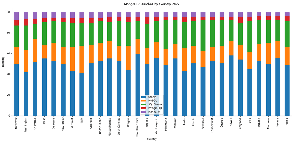
We can delve into the data more, by focusing on one particular country and examine the google searches by city or region. The following looks at the data from USA and gives the rankings for the various states.
pytrends.build_payload(search_list, geo='US')
df_ibr = pytrends.interest_by_region(resolution='COUNTRY', inc_low_vol=True)
df_ibr.sort_values('Oracle', ascending=False).head(20)

df2.reset_index().plot(x='geoName', y=['Oracle', 'MySQL', 'SQL Server', 'PostgreSQL', 'MongoDB'], kind ='bar', stacked=True, title="test")
plt.rcParams["figure.figsize"] = [20, 8]

plt.title("Searches for USA")
plt.xlabel("State")
plt.ylabel("Ranking")


We can find the top related queries and and top queries including the names of each database.
search_list = ["Oracle", "MySQL", "SQL Server", "PostgreSQL", "MongoDB"] #max of 5 values allowed
pytrends.build_payload(search_list, timeframe='today 12-m')

rq = pytrends.related_queries()
rq.values()

#display rising terms
rq.get('Oracle').get('rising')
We can see the top related rising queries for Oracle are about tik tok. No real surprise there!

and the top queries for Oracle included:
rq.get('Oracle').get('top')

This was an interesting exercise to do. I didn’t show all the results, but when you explore the other databases in the list and see the results from those, and then compare them across the five databases you get to see some interesting patterns.

You must be logged in to post a comment.