
SelectAI – Doing something useful
In a previous post, I introduced Select AI and gave examples of how to do some simple things. These included asking it using some natural language questions, to query some data in the Database. That post used both Cohere and OpenAI to process the requests. There were mixed results and some gave a different, somewhat disappointing, outcome. But with using OpenAI the overall outcome was a bit more positive. To build upon the previous post, this post will explore some of the additional features of Select AI, which can give more options for incorporating Select AI into your applications/solutions.
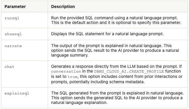
Select AI has five parameters, as shown in the table below. In the previous post, the examples focused on using the first parameter. Although those examples didn’t include the parameter name ‘runsql‘. It is the default parameter and can be excluded from the Select AI statement. Although there were mixed results from using this default parameter ‘runsql’, it is the other parameters that make things a little bit more interesting and gives you opportunities to include these in your applications. In particular, the ‘narrate‘ and ‘explainsql‘ parameters and to a lesser extent the ‘chat‘ parameter. Although for the ‘chat’ parameter there are perhaps slightly easier and more efficient ways of doing this.
Let’s start by looking at the ‘chat‘ parameter. This allows you to ‘chat’ LLM just like you would with ChatGPT and other similar. A useful parameter to set in the CREATE_PROFILE is to set the conversation to TRUE, as that can give more useful results as the conversation develops.
BEGIN
  DBMS_CLOUD_AI.drop_profile(profile_name => 'OPEN_AI');
  DBMS_CLOUD_AI.create_profile(
      profile_name => 'OPEN_AI',
      attributes => '{"provider": "openai",
                      "credential_name": "OPENAI_CRED",
                      "object_list": [{"owner": "SH", "name": "customers"},
                                      {"owner": "SH", "name": "sales"},
                                      {"owner": "SH", "name": "products"},
                                      {"owner": "SH", "name": "countries"},
                                      {"owner": "SH", "name": "channels"},
                                      {"owner": "SH", "name": "promotions"},
                                      {"owner": "SH", "name": "times"}],
        "conversation": "true",        "model":"gpt-3.5-turbo"       }');
END;
There are a few statements I’ve used.
select AI chat who is the president of ireland;
select AI chat what role does NAMA have in ireland;
select AI chat what are the annual revenues of Oracle;
select AI chat who is the largest cloud computing provider;
select AI chat can you rank the cloud providers by income over the last 5 years;
select AI chat what are the benefits of using Oracle Cloud;
As you’d expect the results can be ‘kind of correct’, with varying levels of information given. I’ve tried these using Cohere and OpenAI, and their responses illustrate the need for careful testing and evaluation of the various LLMs to see which one suits your needs.
In my previous post, I gave some examples of using Select AI to query data in the Database based on a natural language request. Select AI takes that request and sends it, along with details of the objects listed in the create_profile, to the LLM. The LLM then sends back the SQL statement, which is then executed in the Database and the results are displayed. But what if you want to see the SQL generated by the LLM. To see the SQL you can use the ‘showsql‘ parameter. Here are a couple of examples:
SQL> select AI showsql how many customers in San Francisco are married;

RESPONSE
_____________________________________________________________________________SELECT COUNT(*) AS total_married_customers
FROM SH.CUSTOMERS c
WHERE c.CUST_CITY = 'San Francisco'
AND c.CUST_MARITAL_STATUS = 'Married'

SQL> select AI what customer is the largest by sales;

   CUST_ID CUST_FIRST_NAME    CUST_LAST_NAME       TOTAL_SALES
__________ __________________ _________________ ______________
     11407 Dora               Rice                   103412.66


SQL> select AI showsql what customer is the largest by sales;

RESPONSE
_____________________________________________________________________________SELECT C.CUST_ID, C.CUST_FIRST_NAME, C.CUST_LAST_NAME, SUM(S.AMOUNT_SOLD) AS TOTAL_SALES
FROM SH.CUSTOMERS C
JOIN SH.SALES S ON C.CUST_ID = S.CUST_ID
GROUP BY C.CUST_ID, C.CUST_FIRST_NAME, C.CUST_LAST_NAME
ORDER BY TOTAL_SALES DESC
FETCH FIRST 1 ROW ONLY
The examples above that illustrate the ‘showsql‘ is kind of interesting. Careful consideration of how and where to use this is needed.
Where things get a little bit more interesting with the ‘narrate‘ parameter, which attempts to narrate or explain the output from the query. There are many use cases where this can be used to supplement existing dashboards, etc. The following are examples of using ‘narrate‘ for the same two queries used above.
SQL> select AI narrate how many customers in San Francisco are married;

RESPONSE
________________________________________________________________
The total number of married customers in San Francisco is 18.


SQL> select AI narrate what customer is the largest by sales;

RESPONSE
_____________________________________________________________________________To find the customer with the largest sales, you can use the following SQL query:

```sql
SELECT c.CUST_FIRST_NAME || ' ' || c.CUST_LAST_NAME AS CUSTOMER_NAME, SUM(s.AMOUNT_SOLD) AS TOTAL_SALES
FROM "SH"."CUSTOMERS" c
JOIN "SH"."SALES" s ON c.CUST_ID = s.CUST_ID
GROUP BY c.CUST_FIRST_NAME, c.CUST_LAST_NAME
ORDER BY TOTAL_SALES DESC
FETCH FIRST 1 ROW ONLY;
```

This query joins the "CUSTOMERS" and "SALES" tables on the customer ID and calculates the total sales for each customer. It then sorts the results in descending order of total sales and fetches only the first row, which represents the customer with the largest sales.

The result will be in the following format:

| CUSTOMER_NAME | TOTAL_SALES |
|---------------|-------------|
| Tess Drumm    | 161882.79   |

In this example, the customer with the largest sales is "Tess Drumm" with a total sales amount of 161,882.79.
Looking at the outputs from using the ‘narrate‘ parameter, we can see the level of detail given and see the potential of including this kind of information in our applications, dashboards, etc. But to use this output some additional filtering and subsetting will need to be performed.
The final parameter is called ‘explainsql‘. While it may not be as useful as the ‘narrate‘ parameter, it does have some potential uses. The ‘explainsql‘ attempts to explain in natural language what a SQL query is attempting to do, based on a natural language statement. Again using the same two examples, we get the following.
SQL> select AI explainsql what customer is the largest by sales;

RESPONSE
_____________________________________________________________________________SELECT C.CUST_ID, C.CUST_FIRST_NAME, C.CUST_LAST_NAME, SUM(S.AMOUNT_SOLD) AS TOTAL_SALES
FROM SH.CUSTOMERS C
JOIN SH.SALES S ON C.CUST_ID = S.CUST_ID
GROUP BY C.CUST_ID, C.CUST_FIRST_NAME, C.CUST_LAST_NAME
ORDER BY TOTAL_SALES DESC
FETCH FIRST 1 ROW ONLY;

Explanation:
- The query selects the customer ID, first name, last name, and the sum of the amount sold from the CUSTOMERS and SALES tables.
- The CUSTOMERS and SALES tables are joined on the CUST_ID column.
- The results are grouped by customer ID, first name, and last name.
- The results are then ordered in descending order by the total sales.
- The FETCH FIRST 1 ROW ONLY clause is used to retrieve only the top row with the highest total sales.

SQL> select AI explainsql how many customers in San Francisco are married;

RESPONSE
_____________________________________________________________________________
SELECT COUNT(*) AS total_married_customers
FROM SH.CUSTOMERS c
WHERE c.CUST_CITY = 'San Francisco'
AND c.CUST_MARITAL_STATUS = 'Married';

This query selects the count of customers who are married and live in San Francisco. The table alias "c" is used for the CUSTOMERS table. The condition "c.CUST_CITY = 'San Francisco'" filters the customers who live in San Francisco, and the condition "c.CUST_MARITAL_STATUS = 'Married'" filters the customers who are married. The result is the total number of married customers in San Francisco.
Check out the other posts about Select AI.
SelectAI – the beginning of a journey
Oracle released Select AI a few months ago, and with any new product it is always a good idea to give it a little time to fix any “bugs” or “features”. To a certain extent, the release of this capability is a long time behind the marketplace. Similar products have been available in different ways, in different products, in different languages, etc for some time now. I’m not going to get into the benefits of this feature/product, as lots have been written about this and most of those are just rehashing the documentation and the marketing materials created for the release. But over all this time, Oracle seems to have been focused on deploying generative AI and LLM related features into their vast collection of applications. Yes, they have done some really cool work with those applications. But during that period the everyday developer, outside of those Apps development teams, has been left waiting for too long to get proper access to this functionality. In most cases, they have gone elsewhere. One thing Oracle does need to address is the public messaging around certain behavioural aspects of Select AI. There has been some contradictory information between what it says in the documentation and what the various Product Managers are saying. This is a problem, as it just confuses customers who will then use something else.
I’m building a particular application that utilizes various OCI products, including some of their AI products, to create a hands-free way of interacting with data and is suitable for those who have various physical and visual impairments. Should I consider including Select AI? Let’s see if it is up to the task.
Let’s get on with setting up and using Select AI. This post focuses on getting it set-up and running with some basic commands, plus a few warnings too as it isn’t all that it’s made out to be! Check out my other posts that explore different aspects (most other posts only show one or two statements), and some of the issues you need to watch out for, as it may not entirely live up to expectations.
The first thing you need to be aware of, this functionality is only available on an ADW/ATP on Oracle Cloud. At some point, we might have it on-premises, but that might be a while coming as I’m sure the developers are still working on improving how it works (and yes it does need some work).
Step 1 – Connect as ADMIN of ADW/ATP
As the ADMIN user for the database, you need to set-up a few things for other users of the Database before they can use Select AI.
Firstly we add the schema which will be using Select AI to the Access Control List. This will allow them to reach things outside of the Database. The following illustrates adding the BRENDAN schema to the list and allowing HTTP calls to the Cohere API interface.
BEGIN
    DBMS_NETWORK_ACL_ADMIN.APPEND_HOST_ACE(
         host => 'api.cohere.ai',
         ace => xs$ace_type(privilege_list => xs$name_list('http'),
         principal_name => 'BRENDAN',
         principal_type => xs_acl.ptype_db)
    );
END;
Next, we need to grant some privileges to some PL/SQL packages.
grant execute on DBMS_CLOUD_AI to BRENDAN;
grant execute on DBMS_CLOUD to BRENDAN;
That’s the admin steps
Step 2 – Connect to your Schema/User – Cohere Example (see OpenAI later in this post)
In my BRENDAN schema, I need to create a Credential.
BEGIN
   -- DBMS_CLOUD.DROP_CREDENTIAL (credential_name => 'COHERE_CRED');

   DBMS_CLOUD.CREATE_CREDENTIAL(
       credential_name => 'COHERE_CRED',
       username => 'COHERE',
       password => '...' );
END;
The … in the above example, indicates where you can place your Cohere API key. It’s very easy to get this and this explains the steps.
Next, you need to create a CLOUD_AI profile.
BEGIN
   --DBMS_CLOUD_AI.drop_profile(profile_name => 'COHERE_AI');

   DBMS_CLOUD_AI.create_profile(
      profile_name => 'COHERE_AI',
      attributes => '{"provider": "cohere",
                      "credential_name": "COHERE_CRED",
                      "object_list": [{"owner": "SH", "name": "customers"},
                                      {"owner": "SH", "name": "sales"},
                                      {"owner": "SH", "name": "products"},
                                      {"owner": "SH", "name": "countries"},
                                      {"owner": "SH", "name": "channels"},
                                      {"owner": "SH", "name": "promotions"},
                                      {"owner": "SH", "name": "times"}]
       }');
END;
When creating the CLOUD_AI profile for your schema, you can list the objects/tables you want to expose to the Cohere or OpenAI models. In theory (so the documentation says) it shares various metadata about these objects/tables, which the models in turn interpret, and use this to formulate their response. I said in theory, as that is what the documentation says, but the PMs on a recent webcast said it did use things like primary keys, foreign keys, etc. There are many other challenges here, and I’ll come back to those at a later time.
At this point, you are all set up to use Select AI.
Step 3 – See if you can get Select AI to work!
Before you can use Select AI, you need to enable it for your session. To do this run,
EXEC DBMS_CLOUD_AI.set_profile('COHERE_AI');If you start a new session/connection or your session/connection gets reset, you will need to run the above command again.
No onto the fun or less fun part. The Fun part is using it and getting results displayed back to you. When this happens (i.e. when it works) it can look like magic is happening. For example here are some commands that worked for me.
select ai how many customers exist;
select AI which customer is the biggest;
select AI what customer is the largest by revenue;
select AI what customer is the largest by sales;
The real challenge with using Select AI is crafting a statement that works i.e. a query is run in the Database and the results are displayed back to you. This can be a real challenge. There are many blog posts out there with lots of examples of using Select AI, along with all the ‘canned’ examples in the documentation and in demos from PMs. I’ve tried all that I could find, and most/all of them didn’t work for me. Something isn’t working correctly behind the scenes. For example here are some examples of statements that didn’t work for me.
select AI how many customers in San Francisco are married;
select AI what is our best selling product by country;
select AI what is our biggest selling product by country;
select AI how many items with the product sub category of Cameras were sold in 1998;
select AI what customer is the biggest;
select AI which customer is the largest by revenue;
Yet some of these statements (above) have been given in docs/posts/demos as working. For a little surprise, have a look at the comment at the bottom of this post.
Don’t let this put you off from trying it. What I’ve shown here is just one part of what Select AI can do. Check out my next post on Select AI where I’ll show examples of the other features, which work and can be used to build some interesting solutions for your users.
Set-up for OpenAI
The steps I’ve given above are for using Cohere. A few others can be used including the popular OpenAI. The setup is very similar to what I’ve shown above and the main difference is the Hostname, OpenAI API key and username. See here for how to get an OpenAI API key.
As ADMIN run.
BEGIN
    DBMS_NETWORK_ACL_ADMIN.APPEND_HOST_ACE(
         host => 'api.openai.com',
         ace  => xs$ace_type(privilege_list => xs$name_list('http'),
                             principal_name => 'BRENDAN',
                             principal_type => xs_acl.ptype_db)
   );
END;
Then in your Schema/user.
BEGIN
   DBMS_CLOUD.DROP_CREDENTIAL (credential_name  => 'OPENAI_CRED');

  DBMS_CLOUD.CREATE_CREDENTIAL(
    credential_name => 'OPENAI_CRED',
    username => '.....',
    password => '...' );
END;
BEGIN
DBMS_CLOUD_AI.drop_profile(profile_name => 'OPEN_AI');
DBMS_CLOUD_AI.create_profile(
profile_name => 'OPEN_AI',
attributes => '{"provider": "openai",
"credential_name": "OPENAI_CRED",
"object_list": [{"owner": "SH", "name": "customers"},
{"owner": "SH", "name": "sales"},
{"owner": "SH", "name": "products"},
{"owner": "SH", "name": "countries"},
{"owner": "SH", "name": "channels"},
{"owner": "SH", "name": "promotions"},
{"owner": "SH", "name": "times"}],
"model":"gpt-3.5-turbo"
}');
END;And then run the following before trying any use Select AI.
EXEC DBMS_CLOUD_AI.set_profile('OPEN_AI');If you look earlier in this post, I listed some questions that couldn’t be answered using Cohere. When I switched to using OpenAPI, all of these worked for me. The question then is, which LLM should you use? based on this simple experiment use Open API and avoid Cohere. But things might be different for you and at a later time when Cohere has time to improve.
Check out the other posts about Select AI.
EU AI Act has been passed by EU parliament
It feels like we’ve been hearing about and talking about the EU AI Act for a very long time now. But on Wednesday 13th March 2024, the EU Parliament finally voted to approve the Act. While this is a major milestone, we haven’t crossed the finish line. There are a few steps to complete, although these are minor steps and are part of the process.

The remaining timeline is:
- The EU AI Act will undergo final linguistic approval by lawyer-linguists in April. This is considered a formality step.
- It will then be published in the Official EU Journal
- 21 days after being published it will come into effect (probably in May)
- The Prohibited Systems provisions will come into force six months later (probably by end of 2024)
- All other provisions in the Act will come into force over the next 2-3 years
If you haven’t already started looking at and evaluating the various elements of AI deployed in your organisation, now is the time to start. It’s time to prepare and explore what changes, if any, you need to make. If you don’t the penalties for non-compliance are hefty, with fines of up to €35 million or 7% of global turnover.
The first thing you need to address is the Prohibited AI Systems and the EU AI Act outlines the following and will need to be addressed before the end of 2024:
- Manipulative and Deceptive Practices: systems that use subliminal techniques to materially distort a person’s decision-making capacity, leading to significant harm. This includes systems that manipulate behaviour or decisions in a way that the individual would not have otherwise made.
- Exploitation of Vulnerabilities: systems that target individuals or groups based on age, disability, or socio-economic status to distort behaviour in harmful ways.
- Biometric Categorisation: systems that categorise individuals based on biometric data to infer sensitive information like race, political opinions, or sexual orientation. This prohibition does not cover any labelling or filtering of lawfully acquired biometric datasets, such as images. There are also exceptions for law enforcement.
- Social Scoring: systems designed to evaluate individuals or groups over time based on their social behaviour or predicted personal characteristics, leading to detrimental treatment.
- Real-time Biometric Identification: The use of real-time remote biometric identification systems in publicly accessible spaces for law enforcement is heavily restricted, with allowances only under narrowly defined circumstances that require judicial or independent administrative approval.
- Risk Assessment in Criminal Offences: systems that assess the risk of individuals committing criminal offences based solely on profiling, except when supporting human assessment already based on factual evidence.
- Facial Recognition Databases: systems that create or expand facial recognition databases through untargeted scraping of images are prohibited.
- Emotion Inference in Workplaces and Educational Institutions: The use of AI to infer emotions in sensitive environments like workplaces and schools is banned, barring exceptions for medical or safety reasons.
In addition to the timeline given above we also have:
- 12 months after entry into force: Obligations on providers of general purpose AI models go into effect. Appointment of member state competent authorities. Annual Commission review of and possible amendments to the list of prohibited AI.
- after 18 months: Commission implementing act on post-market monitoring
- after 24 months: Obligations on high-risk AI systems specifically listed in Annex III, which includes AI systems in biometrics, critical infrastructure, education, employment, access to essential public services, law enforcement, immigration and administration of justice. Member states to have implemented rules on penalties, including administrative fines. Member state authorities to have established at least one operational AI regulatory sandbox. Commission review and possible amendment of the last of high-risk AI systems.
- after 36 months: Obligations for high-rish AI systems that are not prescribed in Annex III but are intended to be used as a safety component of a product, or the AI is itself a product, and the product is required to undergo a third-party conformity assessment under existing specific laws, for example, toys, radio equipment, in vitro diagnostic medical devices, civil aviation security and agricultural vehicles.
The EU has provided an official compliance check that helps identify which parts of the EU AI Act apply in a given use case.
Cohere and OpenAI API Keys
To access and use the Generative AI features in the Oracle Database you’ll need access to the API of a LLM. In this post, I’ll step through what you need to do to get API keys from Cohere and OpenAI. These are the two main LLMs for use with the database and others will be accessible over time.
Cohere API
First, go to the Cohere API Dashboard. You can sign-up using your Google or GitHub accounts to sign in. Or create an account by clicking on Sign-up? (Bottom right-hand corner of page). Fill in your email address and a suitable password. Then confirm your sign-up using the email they just sent to you.

When you sign-up to Cohere, you are initially creating a Trial (Free) account. For now, this will be enough for playing with Select AI. There are some restrictions (shown below) but these might change over time so make sure to check this out.
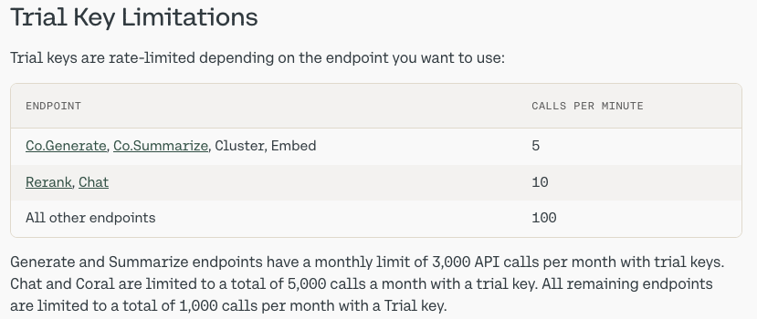
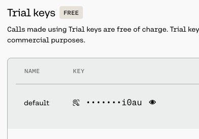
From your Cohere Dashboard, you can access your API key, and use this to set-up your access to the LLM from your remote (app, database, etc) environment. This is a Trial API Key, that is rate-limited, so is kind of ok for testing and evaluation. If you need more, you’ll need to upgrade your account.
Open API
For Open API, you’ll need to create an account – Sign-up here.
Initially, you’ll be set-up with a Trial Account but you may need to upgrade this by depositing some money into your account. The minimum is $10 (plus taxes) and this should be enough to allow you to have a good play with using the API, and only top-up as needed after that, particularly if you go into production use. When you get logged into OpenAI, go to your Dashboard and click on the ‘Create new secret key’ button.

When you’ve obtained the API keys check out my other posts on how to allow access to these from the database and start using the Oracle Select AI features (and other products and code libraries) .
You only need an API key from one of these, but I’ve shown both. This allows you to decide which one you’d like to use.
Check out the other posts about Select AI.
Oracle SQL Dev – VS Code – Recovering Deleted Connections
With the current early release, there is no way to organise your Database connections like you can in the full Oracle SQL Developer. We are told this will/might be possible in a future release but it might be later this year (or longer) before that feature will be available.
In a previous post, I showed how to import your connections from the full SQL Developer into SQL Dev VS Code. While this is a bit of a fudge, yet relatively straight forward to do, you may or may not want all those connections in your SQL Dev VS Code environment. Typically, you will use different tools, such as SQLcl, SQL*Plus, SQL Developer, etc to perform different tasks, and will only want those connections set up in one of those tools.
As shown in my previous post, SQL Dev VS Code and SQLcl share the same set of connections. These connections and their associated files are stored in the same folder on your computer. On my computer/laptop (which is currently a Mac) this connections folder can be found in the $HOME/.dbtools.
I kind of forgot this important little detail and started to clean up my connections in SQL Dev VS Code, but removing some of my old and less frequently used Connections. Only to discover, that these were no longer listed or available to use in SQLcl, using the connmgr command.
The question I had was, How can I recover these connections?
One option was to reimport the connections into SQLcl following the steps given in a previous blog post. When I do that, the connections are refreshed/overwritten in SQLcl, and because of the shared folder will automatically reappear in SQL Dev VS Code the next time I open it or by clicking on the refresh icon in the Connections pane in SQL Dev VS Code.
But was there a simpler solution? Yes there is, so let’s walk through a simple scenario to illustrate what you need to do.
In SQL Dev VS Code, you can delete a connection by right clicking the connection and selecting Delete from the popup menu. You’ll be asked to confirm the deletion of the connection.

Open a Terminal window and go to your $HOME/.dbtools/connections directory.
In this folder, you will see the deleted connections lists with ‘.removed’. These are your deleted connections. Some might have their original connection name with ‘.removed’ and others will have some weird name, for example, ‘zZqtNdeinniqNhofxqNI9Q.removed‘.
To make the deleted connection usable again just rename the directory removing the ‘.removed’ part. For example,
mv B01-Student2-Brendan.removed B01-Student2-BrendanIf you go back to SQL Dev VS Code, the connection will reappear in the list of Connections after about 5 seconds (on my laptop) but if it doesn’t then click on the refresh icon.
Moving Out of the Cloud – or something hybrid – The Key is Managing your Costs Carefully
Over the past decade, we have been hearing the call of the Cloud, from various vendors. The Cloud has provided a wonderful technology shift in the wider IT industry and accelerated the introduction of new technologies and more efficient ways of doing things. There were a lot of promises made or implied in migrating to the Cloud, and these are still being made.
In February 2023, Andy Jassy (CEO of AWS) highlighted: “I think it’s also useful to remember that 90% to 95% of the global IT spend remains on-premises.”. Despite all the talk, pushing customers and customers deciding for themselves to go to the Cloud, there is still a very significant percentage of IT spending remaining on-premises. If you look at the revenue growth of these Cloud providers (Microsoft, Google, AWS and yes even Oracle), if all that revenue equates to just 5-10% of IT spend, just think of the potential revenues if they can convert 1-2% of that spend. It would be Huge!
We have seen lots of competition between the Cloud vendors with multiple price reductions over the last few years. Get the customers to sign up for their Cloud services. They will sign up when things look cheap, but will it remain that way.
In more recent years, say from 2022 onwards, we have seen some questioning the value of going to the Cloud. It seems to get more expensive as time progresses and in some cases receiving surprisingly large Bills. What at first appears to be cheap and quick to spin up new services, turns out to hit the credit card hard at a later time. We have seen many articles by some well-known companies that were early adopters of the Cloud, and have migrated back to being fully on-premises.
The following are some related articles and documentary about the Cloud and exit from the Cloud.
Why companies are leaving the cloud
90-95% of Global IT spend remains on-premises – says Amazon CEO
And check out this documentary from clouded.tv.
Oracle SQL Dev – VS Code – Import connections via SQLcl
I mentioned in my previous post about importing your SQL Developer connections into the VS Code Extension. The following are the steps you need to complete. A more direct method to import directly from SQL Developer will be available in an upcoming extension update.
To complete this migration of your database connects, you’ll need to have SQLcl (SQL Command Line) version 23.3 installed, as it comes with a new Connection Manager feature.
The first step involves exporting your SQL Developer connections. To do this right-click on ‘Oracle Connections’ in SQL Developer, and then select ‘Export Connections’ from the pop-up menu. Select all your connections and then go through the remaining steps of giving a file name, giving a password, and then Finish.


When the file has been created and the connection exported, go open SQLcl (needs to be a minimum of version 23.3), in /nolog mode.
Set the password used for the SQL Developers connections file. In this example ‘MyPassword’ is the password I entered when creating the file.
SQL> secret set mySecret MyPassword
Secret mySecret stored
Now we can import the connections file.
SQL> connmgr import -key mySecret /Users/brendan.tierney/SQLDev-connections.json
Importing connection 23c-VM-STUDENT: Success
Importing connection B01-Student-Admin: Success
Importing connection B01-Student-Brendan: Success
Importing connection Oracle 23c - Docker - SYS: Success
Importing connection Oracle 23c - Docker - HR: Success
Importing connection 23-Free-VM-SYS: Success
Importing connection B01-Student2-Admin: Success
Importing connection 23-Free-VM-STUDENT: Success
Importing connection 23c-VM-SYSTEM: Success
Importing connection Oracle 23c - Docker - System: Success
Importing connection Oracle 23c - Docker - Benchmark: Success
Importing connection 23-Free-VM-SYSTEM: Success
Importing connection 23c-VM-SYS: Success
Importing connection Oracle 23c - Docker - SH: Success
Importing connection 23c-VM-STUDENT2: Success
Importing connection Oracle 23c - Docker - Brendan: Success
Importing connection B01-Student2-Brendan: Success
17 connection(s) processed
If you need to reimport the connections file, you’ll need to use the replace option. Here’s an example.
connmgr import -duplicates replace -key mySecret /Users/brendan.tierney/SQLDev-connections.jsonYou can see above the connections were imported. You can list these by running
SQL> connmgr list
23-Free-VM-STUDENT
23-Free-VM-SYS
23-Free-VM-SYSTEM
...
To connect to one of these connections using its label by running the following, where the label for the connection is in quotes
SQL> connect -name "Oracle 23c - Docker - Brendan"
Connected.

SQL> show connection
COMMAND_PROPERTIES:
 type: STORE
 name: Oracle 23c - Docker - Brendan
 user: brendan
CONNECTION:
 BRENDAN@jdbc:oracle:thin:@//localhost:1521/FREEPDB1
CONNECTION_IDENTIFIER:
 jdbc:oracle:thin:@//localhost:1521/FREEPDB1
CONNECTION_DB_VERSION:
 Oracle Database 23c Free, Release 23.0.0.0.0 - Developer-Release
 Version 23.2.0.0.0
NOLOG:
 false
PRELIMAUTH:
 false
We’ve just imported and verified the import of our SQL Developer connections into SQLcl. The next step is to import them into VS Code. To do this is very easy. If you don’t have VS Code open, open it and the connections will be automatically imported from SQLcl. How easy is that! or if you have VS Code already open just click on the refresh button in the Connections section.
Note: The connections listed in VS code are shared with SQLcl. If you delete any of these connections in VS Code they will be deleted/removed from SQLcl. It’s the one set of connection details being shared by both applications. So some care is needed. I’m sure future releases of the VS Code extension will provide better options for managing your connections.
SQL Developer for VSCode
We now have a new/different tool for developers to access their Oracle Databases. Traditionally, developers have been using Oracle SQL Developer for maybe 20+ years (if you started using Project Raptor). SQL Developer has developed into a bit of a big beast of a tool, with it trying to be everything to everyone including developers, DBAs, and others. But it does seem like SQL Developer might be coming to an end of life, although that could be for some years to come as it is so wildly used. There have been many challenges with SQL Developer over the years and one of the main challenges is getting new developers to use it. From my experience, developers tell me they just didn’t like it, didn’t like the look and feel of it, it was difficult to use, etc., etc. The list would go on and on and most of those developers would prefer to use other tools (for example DBeaver). For those that are terminal/command line only person, you have SQL*Plus and the modern version called SQLCl (SQL Command Line).
But there is a new kid on the block called Oracle SQL Developer Extension for VS Code. Some reports suggest this will be the future, as all future development will be for this new product, and no new development for the original SQL Developer, with only bug fixing being done.
Although Oracle SQL Developer for VS Code might be the future, it has only recently been released and with all new releases, it can be a little limited in functionality. We are told new functionality will be constantly added, maybe on a monthly or quarterly basis, but let’s see. Look at it, as of now (spring 2024) as being a teenager who will mature over time. And with that, Oracle is trying to appeal to a wider set of developers and with the popularity of VS Code it is not surprising they have made this move. VS Code will automatically update the SQL Developer extension as new updates come available.
To install this Oracle SQL Developer for VS Code, just open VS Code, go to the VS Code Marketplace, search for the extension and install. That’s all there is to it.

Oh, and it’s FREE to use. No licence is needed as it comes under the Oracle Free Use Terms Conditions (FUTC) License.
Installing Oracle Developer for VS Code will keep the extension updated automatically for you, so you don’t have to worry about what version you’re on.
Creating a Connection
If you’ve been using the traditional Oracle SQL Developer, you’ll already have some database connections. At the time of writing this post, there is no easy way to import those. Oracle does say, it will be coming soon (hopefully by the time you are reading this post the import feature will be available), but there is a workaround for this but it does involve a slightly complicated process. I’ll give an example in another post.
To manually create a connection, click the Oracle Explore (the Database icon on left-hand side of the screen). This will open a connections section. The top section is labelled SQL Developer and Connections just under it. You can create connections to your Databases here. There is also an Oracle Cloud Infrastructure Connections. I’ll come back to that another time.

Click on the + icon. A screen like the following will open, and you can enter your database connection details there. In this example, I’m creating a connection to a schema on a 23c Oracle Database running on Docker. These are the same connection details you have in SQL Developer.
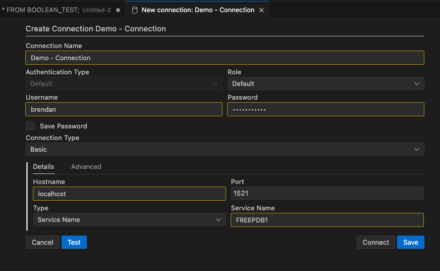
After testing the connection, to make sure it works (a message will display at the bottom of VS Code), you can click on the Save connection. It will now appear in the Databases connections drop-down list and just click on this connection to open it.
Viewing Schema Objects
To see what objects you have in the schema, just click on the connection. It will connect to the schema, and will then display the object list under the schema. You might need to adjust the size of the sections under this Database Connections section to be able to see the full list. Or you might need to close some of them.

SQL Worksheet (writing SQL)
To open a SQL Worksheet, right-click on your Database Connection and click on ‘Open SQL Worksheet’. To run a SQL statement you can click on the Arrow icon in the menu. When you run a SQL statement the results will appear at the bottom of the screen in the Query Results section.

You can run the same query in a couple of other ways. The first is to run it as a script, and the output will be displayed in the ‘Script Output’ tab (beside the ‘Query Results’) and you can also run it in SQLcl (SQL Command Line). SQLcl comes as part of the VS Code extension, although you might have it already installed on your computer, so there might be some slight differences in the version. When you run your SQL query using the SQLcl, it will start SQLcl in the ‘Terminal’ tab, log you into your schema (automatically), run the query and display the results.

There’s a lot to get used to with SQL Developer Extension for VS Code, and there is a lot of functionality yet to come. For a time, you’ll probably end up using both tools. For some, this will not work and they’ll just keep using the traditional SQL Developer. For those people, at some point, you’ll have to make the swap and the sooner you start that transition the easier it will be.
EU AI Regulations: Common Questions and Answers
As the EU AI Regulations move to the next phase, after reaching a political agreement last Nov/Dec 2023, the European Commission has published answers to 28 of the most common questions about the act. These questions are:
- Why do we need to regulate the use of Artificial Intelligence?
- Which risks will the new AI rules address?
- To whom does the AI Act apply?
- What are the risk categories?
- How do I know whether an AI system is high-risk?
- What are the obligations for providers of high-risk AI systems?
- What are examples for high-risk use cases as defined in Annex III?
- How are general-purpose AI models being regulated?
- Why is 10^25 FLOPs an appropriate threshold for GPAI with systemic risks?
- Is the AI Act future-proof?
- How does the AI Act regulate biometric identification?
- Why are particular rules needed for remote biometric identification?
- How do the rules protect fundamental rights?
- What is a fundamental rights impact assessment? Who has to conduct such an assessment, and when?
- How does this regulation address racial and gender bias in AI?
- When will the AI Act be fully applicable?
- How will the AI Act be enforced?
- Why is a European Artificial Intelligence Board needed and what will it do?
- What are the tasks of the European AI Office?
- What is the difference between the AI Board, AI Office, Advisory Forum and Scientific Panel of independent experts?
- What are the penalties for infringement?
- What can individuals do that are affected by a rule violation?
- How do the voluntary codes of conduct for high-risk AI systems work?
- How do the codes of practice for general purpose AI models work?
- Does the AI Act contain provisions regarding environmental protection and sustainability?
- How can the new rules support innovation?
- Besides the AI Act, how will the EU facilitate and support innovation in AI?
- What is the international dimension of the EU’s approach?
This list of Questions and Answers are a beneficial read and clearly addresses common questions you might have seen being addressed in other media outlets. With these being provided and answered by the commission gives us a clear explanation of what is involved.
In addition to the webpage containing these questions and answers, they provide a PDF with them too.
Annual Look at Database Trends (Jan 2024)
Each January I take a little time to look back on the Database market over the previous calendar year. This year I’ll have a look at 2023 (obviously!) and how things have changed and evolved.
In my post from last year (click here) I mentioned the behaviour of some vendors and how they like to be-little other vendors. That kind of behaviour is not really acceptable, but they kept on doing it during 2023 up to a point. That point occurred during the Autumn of 2023. It was during this period there was some degree of consolidation in the IT industry with staff reductions through redundancies, contracts not being renewed, and so on. These changes seemed to have an impact on the messages these companies were putting out and everything seemed to calm down. These staff reductions have continued into 2024.
The first half of the year was generally quiet until we reached the Summer. We then experienced a flurry of activity. The first was the release of the new SQL standard (SQL:2023). There were some discussions about the changes included (for example Property Graph Queries), but the news quickly fizzled out as SQL:2023 was primarily a maintenance release, where the standard was catching up on what many of the database vendors had already implemented over the preceding years. Two new topics seemed to take over the marketing space over the summer months and early autumn. These included LLMs and Vector Databases. Over the Autumn we have seen some releases across vendors incorporating various elements of these and we’ll see more during 2024. Although there have been a lot of marketing on these topics, it still remains to be seen what the real impact of these will be on your average, everyday type of enterprise application. In a similar manner to previous “new killer features” specialised database vendors, we are seeing all the mainstream database vendors incorporating these new features. Just like what has happened over the last 30 years, these specialised vendors will slowly or quickly disappear, as the multi-model database vendors incorporate the features and allow organisations to work with their database rather than having to maintain several different vendors. Another database topic that seemed to attract a lot of attention over the past few years was Distributed SQL (or previously called NewSQL). Again some of the activity around this topic and suppliers seemed to drop off in the second half of 2023. Time will tell what is happening here, maybe it is going through a similar time the NewSQL era had (the previous incarnation). The survivors of that era now call themselves Distributed SQL (Databases), which I think is a better name as it describes what they are doing more clearly. The size of this market is still relatively small. Again time will tell.
There was been some consolidation in the open source vendor market, with some mergers, buyouts, financial difficulties and some shutting down. There have been some high-profile cases not just from the software/support supplier side of things but also from the cloud hosting side of things. Not everyone and not every application can be hosted in the cloud, as Microsoft CEO reported in early 2023 that 90+% of IT spending is still for on-premises. We have also seen several reports and articles of companies reporting their exit from the Cloud (due to costs) and how much they have saved moving back to on-premises data centres.
Two popular sites that constantly monitor the wider internet and judge how popular Databases are globally. These sites are DB-Engines and TOPDB Top Database index. These are well-known and are frequently cited. The image below, based on DB-Engines, shows the position of each Database in the top 20 and compares their position changes to 12 months previously. Here we have a comparison for 2023 and 2022 and the changes in positions. You’ll see there have been no changes in the positions of the top six Databases and minor positional changes for the next five Databases.

Although there has been some positive change for Postgres, given the numbers are based on log scale, this small change is small. The one notable mover in this table is Snowflake, which isn’t surprising really given what they offer and how they’ve been increasing their market share gradually over the years.
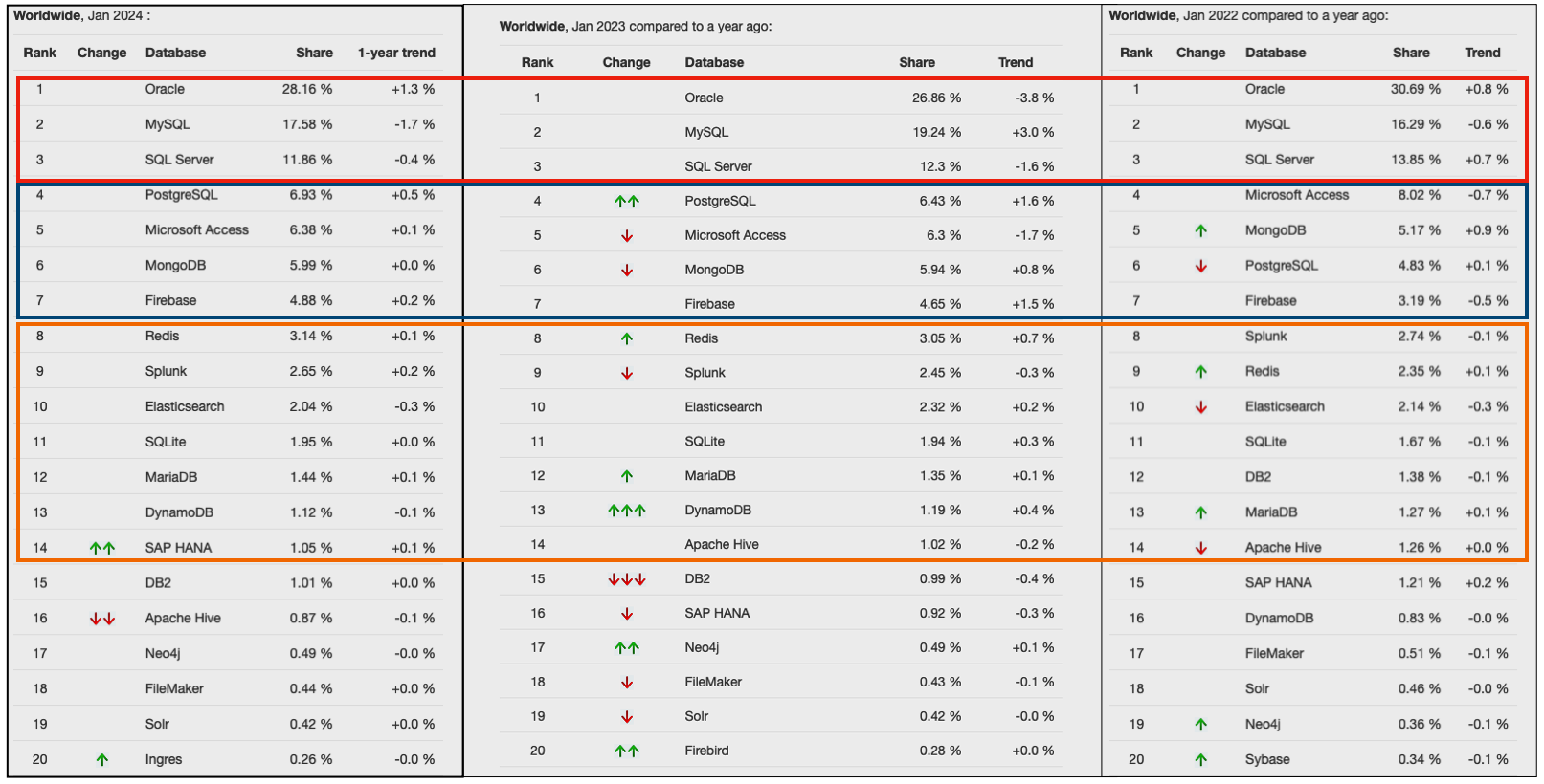
The TOPDB Top Database Index is another popular website and measures the popularity of Databases. It does this in a different way to DB-Engines. It can be an interesting exercise to cross-compare the results between the two websites. The image below compares the results from the past three years from TOPDB Top Database Index. We can see there is very little difference in the positions of most Databases. The point of interest here is the percentage Share of the top ten Databases. Have a look at the Databases that changed by more than one percentage point, and for those Databases (which had a lot of Marketing dollars) which moved very little, despite what some of their associated vendors try to get you to believe.
Changing/Increasing Cell Width in Juypter Notebook
When working with Jupyter Notebook you might notice the cell width can vary from time to time, and mostly when you use different screens, with different resolutions.
This can make your code appear slightly odd on the screen with only a certain amount being used. You can of into the default settings to change the sizing, but this might not suit in most cases.
It would be good to be able to adjust this dynamically. In such a situation, you can use one of the following options.
The first option is to use the IPython option to change the display settings. This first example adjusts everything (menu, toolbar and cells) to 50% of the screen width.
from IPython.display import display, HTML
display(HTML("<style>.container { width:50% !important; }</style>"))
This might not give you the result you want, but it helps to illustrate how to use this command. By changing the percentage, you can get a better outcome. For example, by changing the percentage to 100%.
from IPython.display import display, HTML
display(HTML("<style>.container { width:100% !important; }</style>"))
Keep a careful eye on making these changes, as I’ve found Jupyter stops responding to these changes. A quick refresh of the page will reset everything back to the default settings. Then just run the command you want.
An alternative is to make the changes to the CSS.
from IPython.display import display, HTML

display(HTML(data="""
<style>
    div#notebook-container    { width: 95%; }
    div#menubar-container     { width: 65%; }
    div#maintoolbar-container { width: 99%; }
</style>
"""))
You might want to change those percentages to 100%.
If we need to make the changes permanent we can locate the CSS file: custom.css. Depending on your system it will be located in different places.
For Linux and virtual environments have a look at the following directories.
~/.jupyter/custom/custom.css
Using Python for OCI Vision – Part 1
I’ve written a few blog posts over the past few weeks/months on how to use OCI Vision, which is part of the Oracle OCI AI Services. My blog posts have shown how to get started with OCI Vision, right up to creating your own customer models using this service.
In this post, the first in a series of blog posts, I’ll give you some examples of how to use these custom AI Vision models using Python. Being able to do this, opens the models you create to a larger audience of developers, who can now easily integrate these custom models into their applications.
In a previous post, I covered how to setup and configure your OCI connection. Have a look at that post as you will need to have completed the steps in it before you can follow the steps below.
To inspect the config file we can spool the contents of that file
!cat ~/.oci/config
I’ve hidden some of the details as these are related to my Oracle Cloud accountThis allows us to quickly inspect that we have everything setup correctly.
The next step is to load this config file, and its settings, into our Python environment.
config = oci.config.from_file()

config
We can now list all the projects I’ve created in my compartment for OCI Vision services.
#My Compartment ID
COMPARTMENT_ID = "<compartment-id>"

#List all the AI Vision Projects available in My compartment
response = ai_service_vision_client.list_projects(compartment_id=COMPARTMENT_ID)

#response.data
for item in response.data.items:
    print('- ', item.display_name)
    print('    ProjectId= ', item.id)
    print('')
Which lists the following OCI Vision projects.

We can also list out all the Models in my various projects. When listing these I print out the OCID of each, as this is needed when we want to use one of these models to process an image. I’ve redacted these as there is a minor cost associated with each time these are called.
#List all the AI Vision Models available in My compartment
list_models = ai_service_vision_client.list_models(
    # this is the compartment containing the model
    compartment_id=COMPARTMENT_ID
)

print("Compartment Id=", COMPARTMENT_ID)
print("")
for item in list_models.data.items:
    print('  ', item.display_name, '--', item.model_type)
    print('     OCID= ',item.id)
    print('     ProjectId= ', item.project_id)
    print('')
I’ll have other posts in this series on using the pre-built and custom model to label different image files on my desktop.

You must be logged in to post a comment.