
AI
Exploring Apache Iceberg using PyIceberg – Part 2
Apache Iceberg, an open-source table format that has become the industry standard for data sharing in modern data architectures. In my previous posts on Apache Iceberg I explored the core features of Iceberg Tables and gave examples of using Python code to create, store, add data, read a table and apply filters to an Iceberg Table. In this post I’ll explore some of the more advanced features of interacting with an Iceberg Table, how to add partitioning and how to moved data to a DuckDB database.
Check out the link at the bottom of this post to download the Notebook containing all the PyIceberg code in this post. I had a similar notebook for all the code examples in my previous post. You should check that our first as the examples in the post and notebook are an extension of those.
This post will cover:
- Partitioning an Iceberg Table
- Schema Evolution
- Row Level Operations
- Advanced Scanning & Query Patterns
- DuckDB and Iceberg Tables
Setup & Conguaration
Before we can start on the core aspects of this post, we need to do some basic setup like importing the necessary Python packages, defining the location of the warehouse and catalog and checking the namespace exists. These were created created in the previous post.
import os, pandas as pd, pyarrow as pafrom datetime import datefrom pyiceberg.catalog.sql import SqlCatalogfrom pyiceberg.schema import Schemafrom pyiceberg.types import ( NestedField, LongType, StringType, DoubleType, DateType)from pyiceberg.partitioning import PartitionSpec, PartitionFieldfrom pyiceberg.transforms import ( MonthTransform, IdentityTransform, BucketTransform)WAREHOUSE = "/Users/brendan.tierney/Dropbox/Iceberg-Demo"os.makedirs(WAREHOUSE, exist_ok=True)catalog = SqlCatalog("local", **{ "uri": f"sqlite:///{WAREHOUSE}/catalog.db", "warehouse": f"file://{WAREHOUSE}",})for ns in ["sales_db"]: if ns not in [n[0] for n in catalog.list_namespaces()]: catalog.create_namespace(ns)
Partitioning an Iceberg Table
Partitioning is how Iceberg physically organises data files on disk to enable partition pruning. Partitioning pruning will automactically skip directorys and files that don’t contain the data you are searching for. This can have a significant improvement of query response times.
The following will create a partition table based on the combination of the fiels order_date and region.
# ── Explicit Iceberg schema (gives us full control over field IDs) ─────schema = Schema( NestedField(field_id=1, name="order_id", field_type=LongType(), required=False), NestedField(field_id=2, name="customer", field_type=StringType(), required=False), NestedField(field_id=3, name="product", field_type=StringType(), required=False), NestedField(field_id=4, name="region", field_type=StringType(), required=False), NestedField(field_id=5, name="order_date", field_type=DateType(), required=False), NestedField(field_id=6, name="revenue", field_type=DoubleType(), required=False),)# ── Partition spec: partition by month(order_date) AND identity(region) ─partition_spec = PartitionSpec( PartitionField( source_id=5, # order_date field_id field_id=1000, transform=MonthTransform(), name="order_date_month", ), PartitionField( source_id=4, # region field_id field_id=1001, transform=IdentityTransform(), name="region", ),)tname = ("sales_db", "orders_partitioned")if catalog.table_exists(tname): catalog.drop_table(tname)
Now we can create the table and inspect the details
table = catalog.create_table( tname, schema=schema, partition_spec=partition_spec,)print("Partition spec:", table.spec())Partition spec: [ 1000: order_date_month: month(5) 1001: region: identity(4)]
We can now add data to the partitioned table.
# Write data — Iceberg routes each row to the correct partition directorydf = pd.DataFrame({ "order_id": [1001, 1002, 1003, 1004, 1005, 1006], "customer": ["Alice", "Bob", "Carol", "Dave", "Eve", "Frank"], "product": ["Laptop", "Phone", "Tablet", "Monitor", "Keyboard", "Webcam"], "region": ["EU", "US", "EU", "APAC", "US", "EU"], "order_date": [date(2024,1,15), date(2024,1,20), date(2024,2,3), date(2024,2,20), date(2024,3,5), date(2024,3,12)], "revenue": [1299.99, 1798.00, 549.50, 1197.00, 399.95, 258.00],})table.append(pa.Table.from_pandas(df))
We can inspect the directories and files created. I’ve only include a partical listing below but it should be enough for you to get and idea of what Iceberg as done.
# Verify partition directories were created!find {WAREHOUSE}/sales_db/orders_partitioned/data -type f/Users/brendan.tierney/Dropbox/Iceberg-Demo/sales_db/orders_partitioned/data/region=APAC/order_date_day=2024-04-05/00000-4-0542db6c-f67f-4a26-9012-59d8267b5005.parquet/Users/brendan.tierney/Dropbox/Iceberg-Demo/sales_db/orders_partitioned/data/region=APAC/order_date_day=2024-02-20/00000-2-0542db6c-f67f-4a26-9012-59d8267b5005.parquet/Users/brendan.tierney/Dropbox/Iceberg-Demo/sales_db/orders_partitioned/data/order_date_month=2024-01/region=EU/00000-0-e9ad65a0-c088-46fc-a537-12a6b60b38c5.parquet/Users/brendan.tierney/Dropbox/Iceberg-Demo/sales_db/orders_partitioned/data/order_date_month=2024-01/region=EU/00000-0-1f976101-f836-4db3-bf4a-c0e0cf7dd4c6.parquet/Users/brendan.tierney/Dropbox/Iceberg-Demo/sales_db/orders_partitioned/data/order_date_month=2024-01/region=EU/00000-0-4233dad6-ef48-4ad5-95c9-5842e641fc0f.parquet/Users/brendan.tierney/Dropbox/Iceberg-Demo/sales_db/orders_partitioned/data/order_date_month=2024-01/region=EU/00000-0-b0a10298-d2a6-45b4-a541-9a459e478496.parquet/Users/brendan.tierney/Dropbox/Iceberg-Demo/sales_db/orders_partitioned/data/order_date_month=2024-01/region=US/00000-1-b0a10298-d2a6-45b4-a541-9a459e478496.parquet/Users/brendan.tierney/Dropbox/Iceberg-Demo/sales_db/orders_partitioned/data/order_date_month=2024-01/region=US/00000-1-4233dad6-ef48-4ad5-95c9-5842e641fc0f.parquet/Users/brendan.tierney/Dropbox/Iceberg-Demo/sales_db/orders_partitioned/data/order_date_month=2024-01/region=US/00000-1-1f976101-f836-4db3-bf4a-c0e0cf7dd4c6.parquet/Users/brendan.tierney/Dropbox/Iceberg-Demo/sales_db/orders_partitioned/data/order_date_month=2024-01/region=US/00000-1-e9ad65a0-c088-46fc-a537-12a6b60b38c5.parquet/Users/brendan.tierney/Dropbox/Iceberg-Demo/sales_db/orders_partitioned/data/region=EU/order_date_day=2024-02-03/00000-1-0542db6c-f67f-4a26-9012-59d8267b5005.parquet/Users/brendan.tierney/Dropbox/Iceberg-Demo/sales_db/orders_partitioned/data/region=EU/order_date_day=2024-01-15/00000-0-0542db6c-f67f-4a26-9012-59d8267b5005.parquet/Users/brendan.tierney/Dropbox/Iceberg-Demo/sales_db/orders_partitioned/data/region=EU/order_date_day=2024-04-01/00000-3-0542db6c-f67f-4a26-9012-59d8267b5005.parquet/Users/brendan.tierney/Dropbox/Iceberg-Demo/sales_db/orders_partitioned/data/order_date_month=2024-02/region=APAC/00000-3-b0a10298-d2a6-45b4-a541-9a459e478496.parquet/Users/brendan.tierney/Dropbox/Iceberg-Demo/sales_db/orders_partitioned/data/order_date_month=2024-02/region=APAC/00000-3-e9ad65a0-c088-46fc-a537-12a6b60b38c5.parquet/Users/brendan.tierney/Dropbox/Iceberg-Demo/sales_db/orders_partitioned/data/order_date_month=2024-02/region=APAC/00000-3-4233dad6-ef48-4ad5-95c9-5842e641fc0f.parquet/Users/brendan.tierney/Dropbox/Iceberg-Demo/sales_db/orders_partitioned/data/order_date_month=2024-02/region=APAC/00000-3-1f976101-f836-4db3-bf4a-c0e0cf7dd4c6.parquet
We can change the partictioning specification without rearranging or reorganising the data
from pyiceberg.transforms import DayTransform# Iceberg can change the partition spec without rewriting old data.# Old files keep their original partitioning; new files use the new spec.with table.update_spec() as update: # Upgrade month → day granularity for more recent data update.remove_field("order_date_month") update.add_field( source_column_name="order_date", transform=DayTransform(), partition_field_name="order_date_day", )print("Updated spec:", table.spec())
I’ll leave you to explore the additional directories, files and meta-data files.
#find all files starting from this directory!find {WAREHOUSE}/sales_db/orders_partitioned/data -type f
Schema Evolution
Iceberg tracks every schema version with a numeric ID and never silently breaks existing readers. You can add, rename, and drop columns, change types (safely), and reorder fields, all with zero data rewriting.
#Add new columnsfrom pyiceberg.types import FloatType, BooleanType, TimestampTypeprint("Before:", table.schema())with table.update_schema() as upd: # Add optional columns — old files return NULL for these upd.add_column("discount_pct", FloatType(), "Discount percentage applied") upd.add_column("is_returned", BooleanType(), "True if the order was returned") upd.add_column("updated_at", TimestampType())print("After:", table.schema())Before: table { 1: order_id: optional long 2: customer: optional string 3: product: optional string 4: region: optional string 5: order_date: optional date 6: revenue: optional double}After: table { 1: order_id: optional long 2: customer: optional string 3: product: optional string 4: region: optional string 5: order_date: optional date 6: revenue: optional double 7: discount_pct: optional float (Discount percentage applied) 8: is_returned: optional boolean (True if the order was returned) 9: updated_at: optional timestamp}
We can rename columns. A column rename is a meta-data only change. The Parquet files are untouched. Older readers will still see the previous versions of the column name, whicl new readers will see the new column name.
#rename a columnwith table.update_schema() as upd: upd.rename_column("discount_pct", "discount_percent")print("Updated:", table.schema())Updated: table { 1: order_id: optional long 2: customer: optional string 3: product: optional string 4: region: optional string 5: order_date: optional date 6: revenue: optional double 7: discount_percent: optional float (Discount percentage applied) 8: is_returned: optional boolean (True if the order was returned) 9: updated_at: optional timestamp}
Similarly when dropping a column, it is a meta-data change
#drop a columnwith table.update_schema() as upd: upd.delete_column("updated_at")print("Updated:", table.schema())Updated: table { 1: order_id: optional long 2: customer: optional string 3: product: optional string 4: region: optional string 5: order_date: optional date 6: revenue: optional double 7: discount_percent: optional float (Discount percentage applied) 8: is_returned: optional boolean (True if the order was returned)}
We can see all the different changes or versions of the Iceberg Table schema.
import json, globmeta_files = sorted(glob.glob( f"{WAREHOUSE}/sales_db/orders_partitioned/metadata/*.metadata.json"))with open(meta_files[-1]) as f: meta = json.load(f)print(f"Total schema versions: {len(meta['schemas'])}")for s in meta["schemas"]: print(f" schema-id={s['schema-id']} fields={[f['name'] for f in s['fields']]}")Total schema versions: 4 schema-id=0 fields=['order_id', 'customer', 'product', 'region', 'order_date', 'revenue'] schema-id=1 fields=['order_id', 'customer', 'product', 'region', 'order_date', 'revenue', 'discount_pct', 'is_returned', 'updated_at'] schema-id=2 fields=['order_id', 'customer', 'product', 'region', 'order_date', 'revenue', 'discount_percent', 'is_returned', 'updated_at'] schema-id=3 fields=['order_id', 'customer', 'product', 'region', 'order_date', 'revenue', 'discount_percent', 'is_returned']
Agian if you inspect the directories and files in the warehouse, you’ll see the impact of these changes at the file system level.
#find all files starting from this directory!find {WAREHOUSE}/sales_db/orders_partitioned/data -type f
Row Level Operations
Iceberg v2 introduces two delete file formats that enable row-level mutations without rewriting entire data files immediately — writes stay fast, and reads merge deletes on the fly.
Operations Iceberg Mechanism Write cost Read cost Append New data files only Low Low Delete rows Position or equality delete files Low Medium Update rows Delete + new data file Medium Medium (copy-on-write or merge-on-read) Overwrite Atomic swap of data files Medium Low (replace partition).
from pyiceberg.expressions import EqualTo, In# Delete all orders from the APAC regiontable.delete(EqualTo("region", "APAC"))print(table.scan().to_pandas()) order_id customer product region order_date revenue discount_percent \0 1001 Alice Laptop EU 2024-01-15 1299.99 NaN 1 1002 Bob Phone US 2024-01-20 1798.00 NaN 2 1003 Carol Tablet EU 2024-02-03 549.50 NaN 3 1005 Eve Keyboard US 2024-03-05 399.95 NaN 4 1006 Frank Webcam EU 2024-03-12 258.00 NaN is_returned 0 None 1 None 2 None 3 None 4 None
Also
# Delete specific order IDstable.delete(In("order_id", [1001, 1003]))# Verify — deleted rows are gone from the logical viewdf_after = table.scan().to_pandas()print(f"Rows after delete: {len(df_after)}")print(df_after[["order_id", "customer", "region"]])Rows after delete: 3 order_id customer region0 1002 Bob US1 1005 Eve US2 1006 Frank EU
We can see partiton pruning in action with a scan EqualTo(“region”, “EU”) will skip all data files in region=US/ and region=APAC/ directories entirely — zero bytes read from those files.
Advanced Scanning & Query Processing
The full expression API (And, Or, Not, In, NotIn, StartsWith, IsNull), time travel by snapshot ID, incremental reads between two snapshots for CDC pipelines, and streaming via Arrow RecordBatchReader for out-of-memory processing.
PyIceberg’s scan API supports rich predicate pushdown, snapshot-based time travel, incremental reads between snapshots, and streaming via Arrow record batches.
Let’s start by adding some data back into the table.
df3 = pd.DataFrame({ "order_id": [1001, 1003, 1004, 1006, 1007], "customer": ["Alice", "Carol", "Dave", "Frank", "Grace"], "product": ["Laptop", "Tablet", "Monitor", "Headphones", "Webcam"], "order_date": [ date(2024, 1, 15), date(2024, 2, 3), date(2024, 2, 20), date(2024, 4, 1), date(2024, 4, 5)], "region": ["EU", "EU", "APAC", "EU", "APAC"], "revenue": [1299.99, 549.50, 1197, 498.00, 129.00]})#Add the datatable.append(pa.Table.from_pandas(df3))
Let’s try a query with several predicates.
from pyiceberg.expressions import ( And, Or, Not, EqualTo, NotEqualTo, GreaterThan, GreaterThanOrEqual, LessThan, LessThanOrEqual, In, NotIn, IsNull, IsNaN, StartsWith,)# EU or US orders, revenue > 500, product is not "Keyboard"df_complex = table.scan( row_filter=And( Or( EqualTo("region", "EU"), EqualTo("region", "US"), ), GreaterThan("revenue", 500.0), NotEqualTo("product", "Keyboard"), ), selected_fields=("order_id", "customer", "product", "region", "revenue"),).to_pandas()print(df_complex) order_id customer product region revenue0 1001 Alice Laptop EU 1299.991 1003 Carol Tablet EU 549.502 1002 Bob Phone US 1798.00
Now let’s try a NOT predicate
df_not_in = table.scan( row_filter=Not(In("region", ["US", "APAC"]))).to_pandas()print(df_not_in) order_id customer product region order_date revenue \0 1001 Alice Laptop EU 2024-01-15 1299.99 1 1003 Carol Tablet EU 2024-02-03 549.50 2 1006 Frank Headphones EU 2024-04-01 498.00 3 1006 Frank Webcam EU 2024-03-12 258.00 discount_percent is_returned 0 NaN None 1 NaN None 2 NaN None 3 NaN None
Now filter data with data starting with certain values.
df_starts = table.scan( row_filter=StartsWith("product", "Lap") # matches "Laptop", "Laptop Pro").to_pandas()print(df_starts) order_id customer product region order_date revenue discount_percent \0 1001 Alice Laptop EU 2024-01-15 1299.99 NaN is_returned 0 None
Using the LIMIT function.
df_sample = table.scan(limit=3).to_pandas()print(df_sample) order_id customer product region order_date revenue discount_percent \0 1001 Alice Laptop EU 2024-01-15 1299.99 NaN 1 1003 Carol Tablet EU 2024-02-03 549.50 NaN 2 1004 Dave Monitor APAC 2024-02-20 1197.00 NaN is_returned 0 None 1 None 2 None
We can also perform data streaming.
# Process very large tables without loading everything into memory at oncescan = table.scan(selected_fields=("order_id", "revenue"))total_revenue = 0.0total_rows = 0# to_arrow_batch_reader() returns an Arrow RecordBatchReaderfor batch in scan.to_arrow_batch_reader(): df_chunk = batch.to_pandas() total_revenue += df_chunk["revenue"].sum() total_rows += len(df_chunk)print(f"Total rows: {total_rows}")print(f"Total revenue: ${total_revenue:,.2f}")Total rows: 8Total revenue: $6,129.44
DuckDB and Iceberg Tables
We can register an Iceberg scan plan as a DuckDB virtual table. PyIceberg handles metadata; DuckDB reads the Parquet files.
conn = duckdb.connect()# Expose the scan plan as an Arrow dataset DuckDB can queryscan = table.scan()arrow_dataset = scan.to_arrow() # or to_arrow_batch_reader()conn.register("orders", arrow_dataset)# Full SQL on the tableresult = conn.execute(""" SELECT region, COUNT(*) AS order_count, ROUND(SUM(revenue), 2) AS total_revenue, ROUND(AVG(revenue), 2) AS avg_revenue, ROUND(MAX(revenue) - MIN(revenue), 2) AS revenue_range FROM orders GROUP BY region ORDER BY total_revenue DESC""").df()print(result) region order_count total_revenue avg_revenue revenue_range0 EU 4 2605.49 651.37 1041.991 US 2 2197.95 1098.97 1398.052 APAC 2 1326.00 663.00 1068.00
DuckDB has a native Iceberg extension that reads Parquet files directly.
import duckdb, globconn = duckdb.connect()conn.execute("INSTALL iceberg; LOAD iceberg;")# Enable version guessing for Iceberg tablesconn.execute("SET unsafe_enable_version_guessing = true;")# Point DuckDB at the Iceberg table root directorytable_path = f"{WAREHOUSE}/sales_db/orders_partitioned"df_duck = conn.execute(f""" SELECT * FROM iceberg_scan('{table_path}', allow_moved_paths = true) WHERE revenue > 500 ORDER BY revenue DESC""").df()print(df_duck) order_id customer product region order_date revenue discount_percent \0 1002 Bob Phone US 2024-01-20 1798.00 NaN 1 1001 Alice Laptop EU 2024-01-15 1299.99 NaN 2 1004 Dave Monitor APAC 2024-02-20 1197.00 NaN 3 1003 Carol Tablet EU 2024-02-03 549.50 NaN is_returned 0 <NA> 1 <NA> 2 <NA> 3 <NA>
We can access the data using the time travel Iceberg feature.
# Time travel via DuckDBsnap_id = table.history()[0].snapshot_iddf_tt = conn.execute(f""" SELECT * FROM iceberg_scan( '{table_path}', snapshot_from_id = {snap_id}, allow_moved_paths = true )""").df()print(f"Time travel rows: {len(df_tt)}")Time travel rows: 6
Exploring Apache Iceberg using PyIceberg – Part 1
Apache Iceberg, an open-source table format that has become the industry standard for data sharing in modern data architectures. In a previous post I explored the core feature of Apache Iceberg and compared it with related technologies such as Apache Hudi and Delta Lake.
In this post we’ll look at some of the inital steps to setup and explore Iceberg tables using Python. I’ll have follow-on posts which will explore more advanced features of Apache Iceberg, again using Python. In this post, we’ll explore the following:
- Environmental setup
- Create an Iceberg Table from a Pandas dataframae
- Explore the Iceberg Table and file system
- Appending data and Time Travel
- Read an Iceberg Table into a Pandas dataframe
- Filtered scans with push-down predicates
Check out the link at the bottom of this post to download the Notebook containing all the PyIceberg code.
Environmental setup
Before we can get started with Apache Iceberg, we need to install it in our environment. I’m going with using Python for these blog posts and that means we need to install PyIceberg. In addition to this package, we also need to install pyiceberg-core. This is needed for some additional feature and optimisations of Iceberg.
pip install "pyiceberg[pyiceberg-core]"
This is a very quick install.
Next we need to do some environmental setup, like importing various packages used in the example code, setuping up some directories on the OS where the Iceberg files will be stored, creating a Catalog and a Namespace.
# Import other packages for this Demo Notebookimport pyarrow as paimport pandas as pdfrom datetime import dateimport osfrom pyiceberg.catalog.sql import SqlCatalog#define location for the WAREHOUSE, where the Iceberg files will be locatedWAREHOUSE = "/Users/brendan.tierney/Dropbox/Iceberg-Demo"#create the directory, True = if already exists, then don't report an erroros.makedirs(WAREHOUSE, exist_ok=True)#create a local Catalogcatalog = SqlCatalog( "local", **{ "uri": f"sqlite:///{WAREHOUSE}/catalog.db", "warehouse": f"file://{WAREHOUSE}", })#create a namespace (a bit like a database schema)NAMESPACE = "sales_db"if NAMESPACE not in [ns[0] for ns in catalog.list_namespaces()]: catalog.create_namespace(NAMESPACE)
That’s the initial setup complete.
Create an Iceberg Table from a Pandas dataframe
We can not start creating tables in Iceberg. To do this, the following code examples will initially create a Pandas dataframe, will convert it from table to columnar format (as the data will be stored in Parquet format in the Iceberg table), and then create and populate the Iceberg table.
#create a Pandas DF with some basic data# Create a sample sales DataFramedf = pd.DataFrame({ "order_id": [1001, 1002, 1003, 1004, 1005], "customer": ["Alice", "Bob", "Carol", "Dave", "Eve"], "product": ["Laptop", "Phone", "Tablet", "Monitor", "Keyboard"], "quantity": [1, 2, 1, 3, 5], "unit_price": [1299.99, 899.00, 549.50, 399.00, 79.99], "order_date": [ date(2024, 1, 15), date(2024, 1, 16), date(2024, 2, 3), date(2024, 2, 20), date(2024, 3, 5)], "region": ["EU", "US", "EU", "APAC", "US"]})# Compute total revenue per orderdf["revenue"] = df["quantity"] * df["unit_price"]print(df)print(df.dtypes) order_id customer product quantity unit_price order_date region \0 1001 Alice Laptop 1 1299.99 2024-01-15 EU 1 1002 Bob Phone 2 899.00 2024-01-16 US 2 1003 Carol Tablet 1 549.50 2024-02-03 EU 3 1004 Dave Monitor 3 399.00 2024-02-20 APAC 4 1005 Eve Keyboard 5 79.99 2024-03-05 US revenue 0 1299.99 1 1798.00 2 549.50 3 1197.00 4 399.95 order_id int64customer objectproduct objectquantity int64unit_price float64order_date objectregion objectrevenue float64dtype: object
That’s the Pandas dataframe created. Now we can convert it to columnar format using PyArrow.
#Convert pandas DataFrame → PyArrow Table # PyIceberg writes via Arrow (columnar format), so this step is requiredarrow_table = pa.Table.from_pandas(df)print("Arrow schema:")print(arrow_table.schema)Arrow schema:order_id: int64customer: stringproduct: stringquantity: int64unit_price: doubleorder_date: date32[day]region: stringrevenue: double-- schema metadata --pandas: '{"index_columns": [{"kind": "range", "name": null, "start": 0, "' + 1180
Now we can define the Iceberg table along with the namespace for it.
#Create an Iceberg table from the Arrow schemaTABLE_NAME = (NAMESPACE, "orders")table = catalog.create_table( TABLE_NAME, schema=arrow_table.schema,)tableorders( 1: order_id: optional long, 2: customer: optional string, 3: product: optional string, 4: quantity: optional long, 5: unit_price: optional double, 6: order_date: optional date, 7: region: optional string, 8: revenue: optional double),partition by: [],sort order: [],snapshot: null
The table has been defined in Iceberg and we can see there are no partitions, snapshots, etc. The Iceberg table doesn’t have any data. We can Append the Arrow table data to the Iceberg table.
#add the data to the tabletable.append(arrow_table)#table.append() adds new data files without overwriting existing ones. #Use table.overwrite() to replace all data in a single atomic operation.
We can look at the file system to see what has beeb written.
print(f"Table written to: {WAREHOUSE}/sales_db/orders/")print(f"Snapshot ID: {table.current_snapshot().snapshot_id}")Table written to: /Users/brendan.tierney/Dropbox/Iceberg-Demo/sales_db/orders/Snapshot ID: 3939796261890602539
Explore the Iceberg Table and File System
And Iceberg Table is just a collection of files on the file system, organised into a set of folders. You can look at these using your file system app, or use a terminal window, or in the examples below are from exploring those directories and files from a Jupyter Notebook.
Let’s start at the Warehouse level. This is the topic level that was declared back when the Environment was being setup. Check that out above in the first section.
!ls -l {WAREHOUSE}-rw-r--r--@ 1 brendan.tierney staff 20480 28 Feb 15:26 catalog.dbdrwxr-xr-x@ 3 brendan.tierney staff 96 28 Feb 12:59 sales_db
We can see the catalog file and a directiory for our ‘sales_db’ namespace. When you explore the contents of this file you will find two directorys. These contain the ‘metadata’ and the ‘data’ files. The following list the files found in the ‘data’ directory containing the data and these are stored in parquet format.
!ls -l {WAREHOUSE}/sales_db/orders/data-rw-r--r--@ 1 brendan.tierney staff 3179 28 Feb 15:22 00000-0-357c029e-b420-459b-8248-b1caf3c030ce.parquet-rw-r--r--@ 1 brendan.tierney staff 3307 28 Feb 15:23 00000-0-3fae55d7-1229-448c-9ffb-ae33c77003a3.parquet-rw-r--r--@ 1 brendan.tierney staff 3179 28 Feb 15:03 00000-0-4ec1ef74-cd24-412e-a35f-bcf3d745bf42.parquet-rw-r--r--@ 1 brendan.tierney staff 3179 28 Feb 15:23 00000-0-984ed6d2-4067-43c4-8c11-5f5a96febd24.parquet-rw-r--r-- 1 brendan.tierney staff 3307 28 Feb 15:26 00000-0-a61264e8-b361-490e-90f7-105a33f20dec.parquet-rw-r--r--@ 1 brendan.tierney staff 3307 28 Feb 15:22 00000-0-ac913dfe-548c-4cb3-99aa-4f1332e02248.parquet-rw-r--r--@ 1 brendan.tierney staff 3307 28 Feb 13:00 00000-0-b3fa23ec-79c6-48da-ba81-ba35f25aa7ad.parquet-rw-r--r--@ 1 brendan.tierney staff 3179 28 Feb 15:25 00000-0-d534a298-adab-4744-baa1-198395cc93bd.parquet-rw-r--r--@ 1 brendan.tierney staff 3307 28 Feb 15:21 00000-0-ef5dd6d8-84c0-4860-828e-86e4e175a9eb.parquet-rw-r--r--@ 1 brendan.tierney staff 3179 28 Feb 15:21 00000-0-f108db1c-39f9-4e2b-b825-3e580cccc808.parquet
I’ll leave you to explore the ‘metadata’ directory.
Read the Iceberg Table back into our Environment
To load an Iceberg table into your environment, you’ll need to load the Catalog and then load the table. We have already have the Catalog setup from a previous step, but tht might not be the case in your typical scenario. The following sets up the Catalog and loads the Iceberg table.
#Re-load the catalog and table (as you would in a new session)catalog = SqlCatalog( "local", **{ "uri": f"sqlite:///{WAREHOUSE}/catalog.db", "warehouse": f"file://{WAREHOUSE}", })table2 = catalog.load_table(("sales_db", "orders"))
When we inspect the structure of the Iceberg table we get the names of the columns and the datatypes.
print("--- Iceberg Schema ---")print(table2.schema())--- Iceberg Schema ---table { 1: order_id: optional long 2: customer: optional string 3: product: optional string 4: quantity: optional long 5: unit_price: optional double 6: order_date: optional date 7: region: optional string 8: revenue: optional double}
An Iceberg table can have many snapshots for version control. As we have only added data to the Iceberg table, we should only have one snapshot.
#Snapshot history print("--- Snapshot History ---")for snap in table2.history(): print(snap)--- Snapshot History ---snapshot_id=3939796261890602539 timestamp_ms=1772292384231
We can also inspect the details of the snapshot.
#Current snapshot metadata snap = table2.current_snapshot()print("--- Current Snapshot ---")print(f" ID: {snap.snapshot_id}")print(f" Operation: {snap.summary.operation}")print(f" Records: {snap.summary.get('total-records')}")print(f" Data files: {snap.summary.get('total-data-files')}")print(f" Size bytes: {snap.summary.get('total-files-size')}")--- Current Snapshot --- ID: 3939796261890602539 Operation: Operation.APPEND Records: 5 Data files: 1 Size bytes: 3307
The above shows use there was 5 records added using an Append operation.
An Iceberg table can be partitioned. When we created this table we didn’t specify a partition key, but in an example in another post I’ll give an example of partitioning this table
#Partition spec & sort order print("--- Partition Spec ---")print(table.spec()) # unpartitioned by default--- Partition Spec ---[]
We can also list the files that contain the data for our Iceberg table.
#List physical data files via scanprint("--- Data Files ---")for task in table.scan().plan_files(): print(f" {task.file.file_path}") print(f" record_count={task.file.record_count}, " f"file_size={task.file.file_size_in_bytes} bytes")--- Data Files --- file:///Users/brendan.tierney/Dropbox/Iceberg-Demo/sales_db/orders/data/00000-0-a61264e8-b361-490e-90f7-105a33f20dec.parquet record_count=5, file_size=3307 bytes
Appending Data and Time Travel
Iceberg tables facilitates changes to the schema and data, and to be able to view the data at different points in time. This is refered to as Time Travel. Let’s have a look at an example of this by adding some additional data to the Iceberg table.
# Get and Save the first snapshot id before writing moresnap_v1 = table.current_snapshot().snapshot_id# New batch of orders - 2 new ordersdf2 = pd.DataFrame({ "order_id": [1006, 1007], "customer": ["Frank", "Grace"], "product": ["Headphones", "Webcam"], "quantity": [2, 1], "unit_price": [249.00, 129.00], "order_date": [date(2024, 4, 1), date(2024, 4, 5)], "region": ["EU", "APAC"], "revenue": [498.00, 129.00],})#Add the datatable.append(pa.Table.from_pandas(df2))
We can list the snapshots.
#Get the new snapshot id and check if different to previoussnap_v2 = table.current_snapshot().snapshot_idprint(f"v1 snapshot: {snap_v1}")print(f"v2 snapshot: {snap_v2}")v1 snapshot: 3939796261890602539v2 snapshot: 8666063993760292894
and we can see how see how many records are in each Snapshot, using Time Travel.
#Time travel: read the ORIGINAL 5-row tabledf_v1 = table.scan(snapshot_id=snap_v1).to_pandas()print(f"Snapshot v1 — {len(df_v1)} rows")#Current snapshot has all 7 rowsdf_v2 = table.scan().to_pandas()print(f"Snapshot v2 — {len(df_v2)} rows")Snapshot v1 — 5 rowsSnapshot v2 — 7 rows
If you inspect the file system, in the data and metadata dirctories, you will notices some additional files.
!ls -l {WAREHOUSE}/sales_db/orders/data!ls -l {WAREHOUSE}/sales_db/orders/metadata
Read an Iceberg Table into a Pandas dataframe
To load the Iceberg table into a Pandas dataframe we can
pd_df = table2.scan().to_pandas()
or we can use the Pandas package fuction
df = pd.read_iceberg("orders", "catalog")
Filtered scans with push-down predicates
PyIceberg provides a fluent scan API. You can read the full table or push down filters, column projections, and row limits — all evaluated at the file level.
Filtered Scan with Push Down Predicates
from pyiceberg.expressions import ( EqualTo, GreaterThanOrEqual, And)# Only EU orders with revenue above €1000df_filtered = ( table2.scan( row_filter=And( EqualTo("region", "EU"), GreaterThanOrEqual("revenue", 1000.0), ) ).to_pandas() )print(df_filtered) order_id customer product quantity unit_price order_date region revenue0 1001 Alice Laptop 1 1299.99 2024-01-15 EU 1299.99
Column Projection – select specific columns
# Only fetch the columns you need — saves I/Odf_slim = ( table2.scan(selected_fields=("order_id", "customer", "revenue")) .to_pandas() )print(df_slim) order_id customer revenue0 1001 Alice 1299.991 1002 Bob 1798.002 1003 Carol 549.503 1004 Dave 1197.004 1005 Eve 399.95
We can also use Arrow for more control.
arrow_result = table2.scan().to_arrow()print(arrow_result.schema)df_from_arrow = arrow_result.to_pandas(timestamp_as_object=True)print(df_from_arrow.head())
order_id: int64
customer: string
product: string
quantity: int64
unit_price: double
order_date: date32[day]
region: string
revenue: double
   order_id customer   product  quantity  unit_price  order_date region  \
0      1001    Alice    Laptop         1     1299.99  2024-01-15     EU
1      1002      Bob     Phone         2      899.00  2024-01-16     US
2      1003    Carol    Tablet         1      549.50  2024-02-03     EU
3      1004     Dave   Monitor         3      399.00  2024-02-20   APAC
4      1005      Eve  Keyboard         5       79.99  2024-03-05     US

   revenue
0  1299.99
1  1798.00
2   549.50
3  1197.00
4   399.95
I’ve put all of the above into a Juputer Notebook. You can download this from here, and you can use it for your explorations of Apache Iceberg.
Check out my next post of Apache Iceberg to see my Python code on explore some additional, and advanced features of Apache Iceberg.
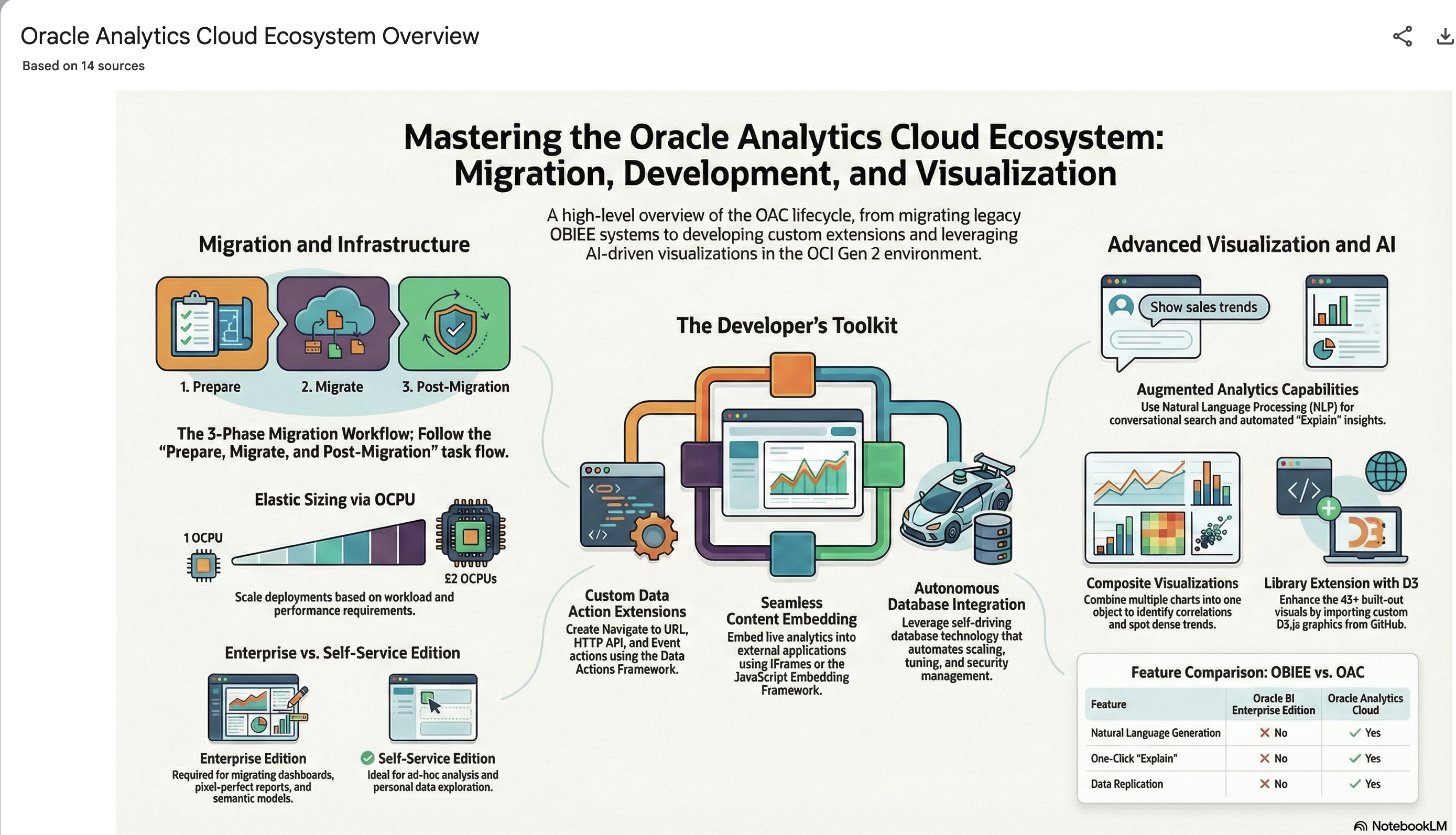
Using NotebookLM to help with understanding Oracle Analytics Cloud or any other product
Over the past few months, we’ve seen a plethora of new LLM related products/agents being released. One such one is NotebookLM from Google. The offical description say “NotebookLM is an AI-powered research and note-taking tool from Google Labs that allows users to ground a large language model (like Gemini) in their own documents, such as PDFs, Google Docs, website URLs, or audio, acting as a personal, intelligent research assistant. It facilitates summarizing, analyzing, and querying information within these specific sources to create study guides, outlines, and, notably, “Audio Overviews” (podcast-style summaries)”
Let’s have a look at using NotebookLM to help with answering questions and how it can help with understanding Oracle Analytics Cloud (OAC).

Yes, you’ll need a Google account, and Yes you need to be OK with uploading your documents to NotebookLM. Make sure you are not breaking any laws (IP, GDPR, etc). It’s really easy to create your first notebook. Simply click on ‘Create new notebook’.
When the notebook opens, you can add your documents and webpages to the notebook. These can be documents in PDF, audio, text, etc to the notebook repository. Currently, there seems to be a limit of 50 documents and webpages that can be added.
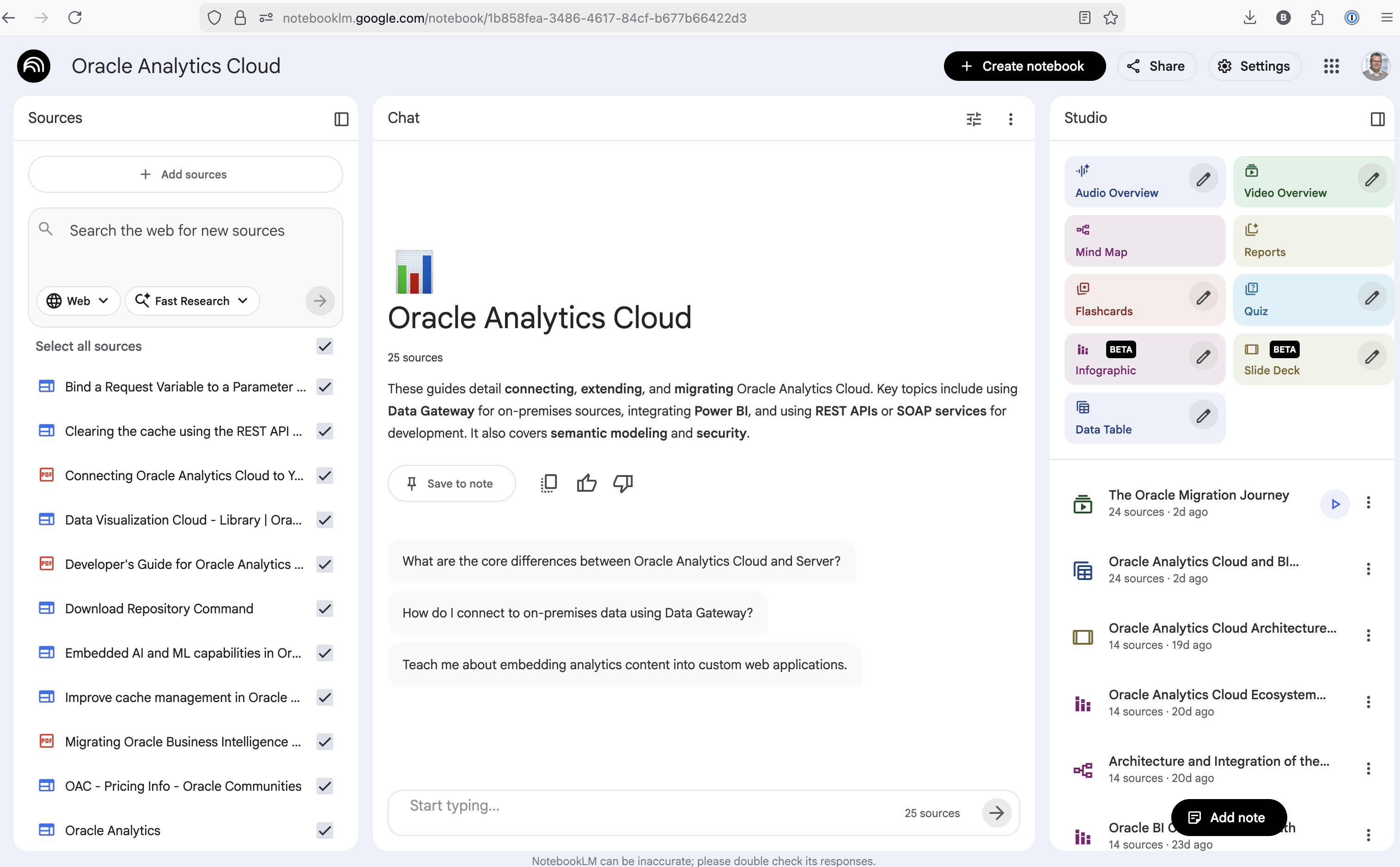
The main part of the NotebookLM provides a chatbot where you can ask questions, and the NotebookLM will search through the documents and webpages to formulate an answer. In addition to this, there are features that allow you to generate Audio Overview, Video Overview, Mind Map, Reports, Flashcards, Quiz, Infographic, Slide Deck and a Data Table.
Before we look at some of these and what they have created for Oracle Analytics Cloud, there is a small warning. Some of these can take a long time to complete, that is, if they complete. I’ve had to run some of these features multiple times to get them to create. I’ve run all of the features, and the output from these can be seen on the right-hand side of the above image.
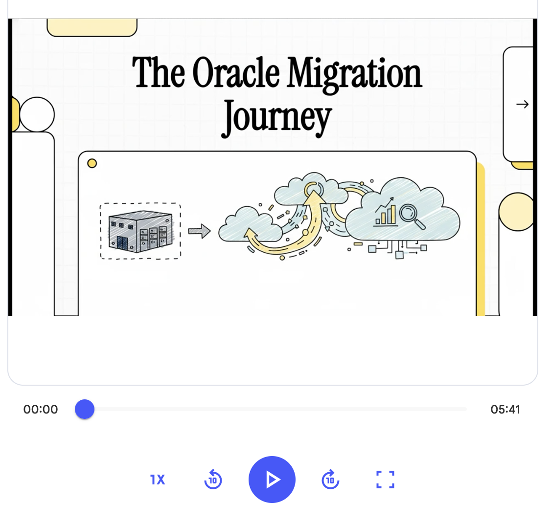
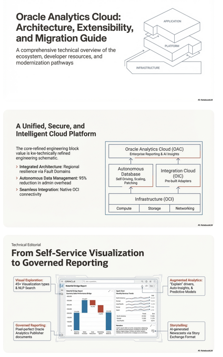
It created a 15-slide presentation on Oracle Analytics Cloud and its various features, and a five minute video on migrating OAC.
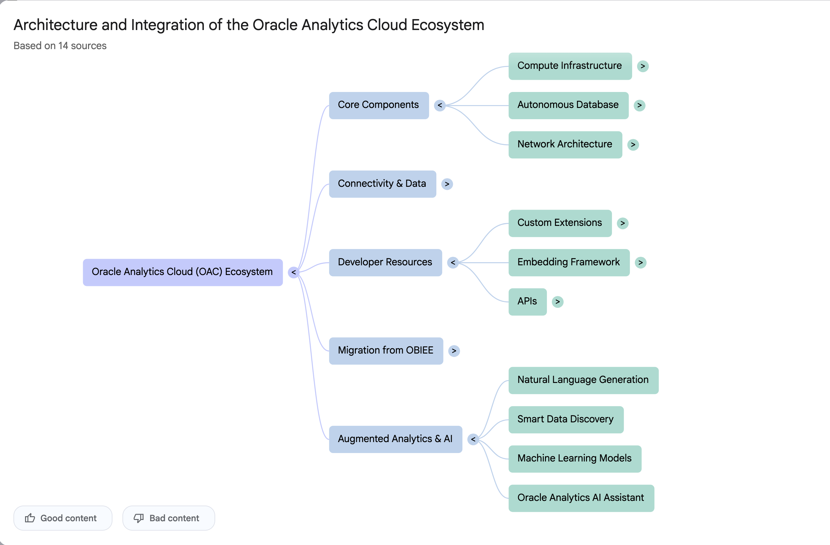
It also created a Mind-map, and an Infographic.
OCI Text to Speech example
In this post, I’ll walk through the steps to get a very simple example of Text-to-Speech working. This example builds upon my previous posts on OCI Language, OCI Speech and others, so make sure you check out those posts.
The first thing you need to be aware of, and to check, before you proceed, is whether the Text-to-Speech is available in your region. At the time of writing, this feature was only available in Phoenix, which is one of the cloud regions I have access to. There are plans to roll it out to other regions, but I’m not aware of the timeline for this. Although you might see Speech listed on your AI menu in OCI, that does not guarantee the Text-to-Speech feature is available. What it does mean is the text trans scribing feature is available.
So if Text-to-Speech is available in your region, the following will get you up and running.
The first thing you need to do is read in the Config file from the OS.
#initial setup, read Config file, create OCI Client
import oci
from oci.config import from_file
##########
from oci_ai_speech_realtime import RealtimeSpeechClient, RealtimeSpeechClientListener
from oci.ai_speech.models import RealtimeParameters
##########

CONFIG_PROFILE = "DEFAULT"
config = oci.config.from_file('~/.oci/config', profile_name=CONFIG_PROFILE)
###
ai_speech_client = ai_speech_client = oci.ai_speech.AIServiceSpeechClient(config)
###
print(config)
### Update region to point to Phoenix
config.update({'region':'us-phoenix-1'})
A simple little test to see if the Text-to-Speech feature is enabled for your region is to display the available list of voices.
list_voices_response = ai_speech_client.list_voices(
    compartment_id=COMPARTMENT_ID,
    display_name="Text-to-Speech")
#    opc_request_id="1GD0CV5QIIS1RFPFIOLF<unique_ID>")

# Get the data from response
print(list_voices_response.data)
This produces a long json object with many characteristics of the available voices. A simpler listing gives the names and gender)
for i in range(len(list_voices_response.data.items)):
    print(list_voices_response.data.items[i].display_name + ' [' + list_voices_response.data.items[i].gender + ']\t' + list_voices_response.data.items[i].language_description )
------
Brian [MALE]	English (United States)
Annabelle [FEMALE]	English (United States)
Bob [MALE]	English (United States)
Stacy [FEMALE]	English (United States)
Phil [MALE]	English (United States)
Cindy [FEMALE]	English (United States)
Brad [MALE]	English (United States)
Richard [MALE]	English (United States)
Now lets setup a Text-to-Speech example using the simple text, Hello. My name is Brendan and this is an example of using Oracle OCI Speech service. First lets define a function to save the audio to a file.
def save_audi_response(data):
    with open(filename, 'wb') as f:
        for b in data.iter_content():
            f.write(b)
    f.close()
We can now establish a connection, define the text, call the OCI Speech function to create the audio, and then to save the audio file.
import IPython.display as ipd

# Initialize service client with default config file
ai_speech_client = oci.ai_speech.AIServiceSpeechClient(config)

TEXT_DEMO = "Hello. My name is Brendan and this is an example of using Oracle OCI Speech service"

#speech_response = ai_speech_client.synthesize_speech(compartment_id=COMPARTMENT_ID)

speech_response = ai_speech_client.synthesize_speech(
    synthesize_speech_details=oci.ai_speech.models.SynthesizeSpeechDetails(
        text=TEXT_DEMO,
        is_stream_enabled=True,
        compartment_id=COMPARTMENT_ID,

        configuration=oci.ai_speech.models.TtsOracleConfiguration(
            model_family="ORACLE",
            model_details=oci.ai_speech.models.TtsOracleTts2NaturalModelDetails(
                model_name="TTS_2_NATURAL",
                voice_id="Annabelle"),
            speech_settings=oci.ai_speech.models.TtsOracleSpeechSettings(
                text_type="SSML",
                sample_rate_in_hz=18288,
                output_format="MP3",
                speech_mark_types=["WORD"])),

        audio_config=oci.ai_speech.models.TtsBaseAudioConfig(config_type="BASE_AUDIO_CONFIG") #, save_path='I'm not sure what this should be')
    ) )

# Get the data from response
#print(speech_response.data)
save_audi_response(speech_response.data)Unlock Text Analytics with Oracle OCI Python – Part 2
This is my second post on using Oracle OCI Language service to perform Text Analytics. These include Language Detection, Text Classification, Sentiment Analysis, Key Phrase Extraction, Named Entity Recognition, Private Data detection and masking, and Healthcare NLP.
In my Previous post (Part 1), I covered examples on Language Detection, Text Classification and Sentiment Analysis.
In this post (Part 2), I’ll cover:
- Key Phrase
- Named Entity Recognition
- Detect private information and marking
Make sure you check out Part 1 for details on setting up the client and establishing a connection. These details are omitted in the examples below.
Key Phrase Extraction
With Key Phrase Extraction, it aims to identify the key works and/or phrases from the text. The keywords/phrases are selected based on what are the main topics in the text along with the confidence score. The text is parsed to extra the words/phrase that are important in the text. This can aid with identifying the key aspects of the document without having to read it. Care is needed as these words/phrases do not represent the meaning implied in the text.
Using some of the same texts used in Part-1, let’s see what gets generated for the text about a Hotel experience.
t_doc = oci.ai_language.models.TextDocument(
    key="Demo",
    text="This hotel is a bad place, I would strongly advise against going there. There was one helpful member of staff",
    language_code="en")

key_phrase = ai_language_client.batch_detect_language_key_phrases((oci.ai_language.models.BatchDetectLanguageKeyPhrasesDetails(documents=[t_doc])))

print(key_phrase.data)
print('==========')
for i in range(len(key_phrase.data.documents)):
        for j in range(len(key_phrase.data.documents[i].key_phrases)):
            print("phrase: ", key_phrase.data.documents[i].key_phrases[j].text +' [' + str(key_phrase.data.documents[i].key_phrases[j].score) + ']')
{
"documents": [
{
"key": "Demo",
"key_phrases": [
{
"score": 0.9998106383818767,
"text": "bad place"
},
{
"score": 0.9998106383818767,
"text": "one helpful member"
},
{
"score": 0.9944029848214838,
"text": "staff"
},
{
"score": 0.9849306609397931,
"text": "hotel"
}
],
"language_code": "en"
}
],
"errors": []
}
==========
phrase: bad place [0.9998106383818767]
phrase: one helpful member [0.9998106383818767]
phrase: staff [0.9944029848214838]
phrase: hotel [0.9849306609397931]The output from the Key Phrase Extraction is presented into two formats about. The first is the JSON object returned from the function, containing the phrases and their confidence score. The second (below the ==========) is a formatted version of the same JSON object but parsed to extract and present the data in a more compact manner.
The next piece of text to be examined is taken from an article on the F1 website about a change of divers.
text_f1 = "Red Bull decided to take swift action after Liam Lawsons difficult start to the 2025 campaign, demoting him to Racing Bulls and promoting Yuki Tsunoda to the senior team alongside reigning world champion Max Verstappen. F1 Correspondent Lawrence Barretto explains why… Sergio Perez had endured a painful campaign that saw him finish a distant eighth in the Drivers Championship for Red Bull last season – while team mate Verstappen won a fourth successive title – and after sticking by him all season, the team opted to end his deal early after Abu Dhabi finale."

t_doc = oci.ai_language.models.TextDocument(
    key="Demo",
    text=text_f1,
    language_code="en")

key_phrase = ai_language_client.batch_detect_language_key_phrases(oci.ai_language.models.BatchDetectLanguageKeyPhrasesDetails(documents=[t_doc]))
print(key_phrase.data)
print('==========')
for i in range(len(key_phrase.data.documents)):
        for j in range(len(key_phrase.data.documents[i].key_phrases)):
            print("phrase: ", key_phrase.data.documents[i].key_phrases[j].text +' [' + str(key_phrase.data.documents[i].key_phrases[j].score) + ']')
I won’t include all the output and the following shows the key phrases in the compact format
phrase:  red bull [0.9991468440416812]
phrase:  swift action [0.9991468440416812]
phrase:  liam lawsons difficult start [0.9991468440416812]
phrase:  2025 campaign [0.9991468440416812]
phrase:  racing bulls [0.9991468440416812]
phrase:  promoting yuki tsunoda [0.9991468440416812]
phrase:  senior team [0.9991468440416812]
phrase:  sergio perez [0.9991468440416812]
phrase:  painful campaign [0.9991468440416812]
phrase:  drivers championship [0.9991468440416812]
phrase:  red bull last season [0.9991468440416812]
phrase:  team mate verstappen [0.9991468440416812]
phrase:  fourth successive title [0.9991468440416812]
phrase:  all season [0.9991468440416812]
phrase:  abu dhabi finale [0.9991468440416812]
phrase:  team [0.9420016064526977]
While some aspects of this is interesting, care is needed to not overly rely upon it. It really depends on the usecase.
Named Entity Recognition
For Named Entity Recognition is a natural language process for finding particular types of entities listed as words or phrases in the text. The named entities are a defined list of items. For OCI Language there is a list available here. Some named entities have a sub entities. The return JSON object from the function has a format like the following.
{
  "documents": [
    {
      "entities": [
        {
          "length": 5,
          "offset": 5,
          "score": 0.969588577747345,
          "sub_type": "FACILITY",
          "text": "hotel",
          "type": "LOCATION"
        },
        {
          "length": 27,
          "offset": 82,
          "score": 0.897526216506958,
          "sub_type": null,
          "text": "one helpful member of staff",
          "type": "QUANTITY"
        }
      ],
      "key": "Demo",
      "language_code": "en"
    }
  ],
  "errors": []
}
For each named entity discovered the returned object will contain the Text identifed, the Entity Type, the Entity Subtype, Confidence Score, offset and length.
Using the text samples used previous, let’s see what gets produced. The first example is for the hotel review.
t_doc = oci.ai_language.models.TextDocument(
    key="Demo",
    text="This hotel is a bad place, I would strongly advise against going there. There was one helpful member of staff",
    language_code="en")

named_entities = ai_language_client.batch_detect_language_entities(
            batch_detect_language_entities_details=oci.ai_language.models.BatchDetectLanguageEntitiesDetails(documents=[t_doc]))

for i in range(len(named_entities.data.documents)):
        for j in range(len(named_entities.data.documents[i].entities)):
            print("Text: ", named_entities.data.documents[i].entities[j].text, ' [' + named_entities.data.documents[i].entities[j].type + ']'
                 + '[' + str(named_entities.data.documents[i].entities[j].sub_type) + ']' + '{offset:'
                 + str(named_entities.data.documents[i].entities[j].offset) + '}')
Text: hotel [LOCATION][FACILITY]{offset:5}
Text: one helpful member of staff [QUANTITY][None]{offset:82}The last two lines above are the formatted output of the JSON object. It contains two named entities. The first one is for the text “hotel” and it has a Entity Type of Location, and a Sub Entitity Type of Location. The second named entity is for a long piece of string and for this it has a Entity Type of Quantity, but has no Sub Entity Type.
Now let’s see what is creates for the F1 text. (the text has been given above and the code is very similar/same as above).
Text:  Red Bull  [ORGANIZATION][None]{offset:0}
Text:  swift  [ORGANIZATION][None]{offset:25}
Text:  Liam Lawsons  [PERSON][None]{offset:44}
Text:  2025  [DATETIME][DATE]{offset:80}
Text:  Yuki Tsunoda  [PERSON][None]{offset:138}
Text:  senior  [QUANTITY][AGE]{offset:158}
Text:  Max Verstappen  [PERSON][None]{offset:204}
Text:  F1  [ORGANIZATION][None]{offset:220}
Text:  Lawrence Barretto  [PERSON][None]{offset:237}
Text:  Sergio Perez  [PERSON][None]{offset:269}
Text:  campaign  [EVENT][None]{offset:304}
Text:  eighth in the  [QUANTITY][None]{offset:343}
Text:  Drivers Championship  [EVENT][None]{offset:357}
Text:  Red Bull  [ORGANIZATION][None]{offset:382}
Text:  Verstappen  [PERSON][None]{offset:421}
Text:  fourth successive title  [QUANTITY][None]{offset:438}
Text:  Abu Dhabi  [LOCATION][GPE]{offset:545}
Detect Private Information and Marking
The ability to perform data masking has been available in SQL for a long time. There are lots of scenarios where masking is needed and you are not using a Database or not at that particular time.
With Detect Private Information or Personal Identifiable Information the OCI AI function search for data that is personal and gives you options on how to present this back to the users. Examples of the types of data or Entity Types it will detect include Person, Adddress, Age, SSN, Passport, Phone Numbers, Bank Accounts, IP Address, Cookie details, Private and Public keys, various OCI related information, etc. The list goes on. Check out the documentation for more details on these. Unfortunately the documentation for how the Python API works is very limited.
The examples below illustrate some of the basic options. But there is lots more you can do with this feature like defining you own rules.
For these examples, I’m going to use the following text which I’ve assigned to a variable called text_demo.
Hi Martin. Thanks for taking my call on 1/04/2025. Here are the details you requested. My Bank Account Number is 1234-5678-9876-5432 and my Bank Branch is Main Street, Dublin. My Date of Birth is 29/02/1993 and I’ve been living at my current address for 15 years. Can you also update my email address to brendan.tierney@email.com. If toy have any problems with this you can contact me on +353-1-493-1111. Thanks for your help. Brendan.
m_mode = {"ALL":{"mode":'MASK'}}

t_doc = oci.ai_language.models.TextDocument(key="Demo", text=text_demo,language_code="en")

pii_entities = ai_language_client.batch_detect_language_pii_entities(oci.ai_language.models.BatchDetectLanguagePiiEntitiesDetails(documents=[t_doc], masking=m_mode))

print(text_demo)
print('--------------------------------------------------------------------------------')
print(pii_entities.data.documents[0].masked_text)
print('--------------------------------------------------------------------------------')
for i in range(len(pii_entities.data.documents)):
        for j in range(len(pii_entities.data.documents[i].entities)):
            print("phrase: ", pii_entities.data.documents[i].entities[j].text +' [' + str(pii_entities.data.documents[i].entities[j].type) + ']')
Hi Martin. Thanks for taking my call on 1/04/2025. Here are the details you requested. My Bank Account Number is 1234-5678-9876-5432 and my Bank Branch is Main Street, Dublin. My Date of Birth is 29/02/1993 and I've been living at my current address for 15 years. Can you also update my email address to brendan.tierney@email.com. If toy have any problems with this you can contact me on +353-1-493-1111. Thanks for your help. Brendan.
--------------------------------------------------------------------------------
Hi ******. Thanks for taking my call on *********. Here are the details you requested. My Bank Account Number is ******************* and my Bank Branch is Main Street, Dublin. My Date of Birth is ********** and I've been living at my current address for ********. Can you also update my email address to *************************. If toy have any problems with this you can contact me on ***************. Thanks for your help. *******.
--------------------------------------------------------------------------------
phrase:  Martin [PERSON]
phrase:  1/04/2025 [DATE_TIME]
phrase:  1234-5678-9876-5432 [CREDIT_DEBIT_NUMBER]
phrase:  29/02/1993 [DATE_TIME]
phrase:  15 years [DATE_TIME]
phrase:  brendan.tierney@email.com [EMAIL]
phrase:  +353-1-493-1111 [TELEPHONE_NUMBER]
phrase:  Brendan [PERSON]
The above this the basic level of masking.
A second option is to use the REMOVE mask. For this, change the mask format to the following.
m_mode = {"ALL":{'mode':'REMOVE'}} For this option the indentified information is removed from the text.
Hi . Thanks for taking my call on . Here are the details you requested. My Bank Account Number is  and my Bank Branch is Main Street, Dublin. My Date of Birth is  and I've been living at my current address for . Can you also update my email address to . If toy have any problems with this you can contact me on . Thanks for your help. .
--------------------------------------------------------------------------------
phrase:  Martin [PERSON]
phrase:  1/04/2025 [DATE_TIME]
phrase:  1234-5678-9876-5432 [CREDIT_DEBIT_NUMBER]
phrase:  29/02/1993 [DATE_TIME]
phrase:  15 years [DATE_TIME]
phrase:  brendan.tierney@email.com [EMAIL]
phrase:  +353-1-493-1111 [TELEPHONE_NUMBER]
phrase:  Brendan [PERSON]
For the REPLACE option we have.
m_mode = {"ALL":{'mode':'REPLACE'}} Which gives us the following, where we can see the key information is removed and replace with the name of Entity Type.
Hi <PERSON>. Thanks for taking my call on <DATE_TIME>. Here are the details you requested. My Bank Account Number is <CREDIT_DEBIT_NUMBER> and my Bank Branch is Main Street, Dublin. My Date of Birth is <DATE_TIME> and I've been living at my current address for <DATE_TIME>. Can you also update my email address to <EMAIL>. If toy have any problems with this you can contact me on <TELEPHONE_NUMBER>. Thanks for your help. <PERSON>.
--------------------------------------------------------------------------------
phrase:  Martin [PERSON]
phrase:  1/04/2025 [DATE_TIME]
phrase:  1234-5678-9876-5432 [CREDIT_DEBIT_NUMBER]
phrase:  29/02/1993 [DATE_TIME]
phrase:  15 years [DATE_TIME]
phrase:  brendan.tierney@email.com [EMAIL]
phrase:  +353-1-493-1111 [TELEPHONE_NUMBER]
phrase:  Brendan [PERSON]
We can also change the character used for the masking. In this example we change the masking character to + symbol.
m_mode = {"ALL":{'mode':'MASK','maskingCharacter':'+'}} Hi ++++++. Thanks for taking my call on +++++++++. Here are the details you requested. My Bank Account Number is +++++++++++++++++++ and my Bank Branch is Main Street, Dublin. My Date of Birth is ++++++++++ and I've been living at my current address for ++++++++. Can you also update my email address to +++++++++++++++++++++++++. If toy have any problems with this you can contact me on +++++++++++++++. Thanks for your help. +++++++.I mentioned at the start of this section there was lots of options available to you, including defining your own rules, using regular expressions, etc. Let me know if you’re interested in exploring some of these and I can share a few more examples.
Unlock Text Analytics with Oracle OCI Python – Part 1
Oracle OCI has a number of features that allows you to perform Text Analytics such as Language Detection, Text Classification, Sentiment Analysis, Key Phrase Extraction, Named Entity Recognition, Private Data detection and masking, and Healthcare NLP.

While some of these have particular (and in some instances limited) use cases, the following examples will illustrate some of the main features using the OCI Python library. Why am I using Python to illustrate these? This is because most developers are using Python to build applications.
In this post, the Python examples below will cover the following:
- Language Detection
- Text Classification
- Sentiment Analysis
In my next post on this topic, I’ll cover:
- Key Phrase
- Named Entity Recognition
- Detect private information and marking
Before you can use any of the OCI AI Services, you need to set up a config file on your computer. This will contain the details necessary to establish a secure connection to your OCI tendency. Check out this blog post about setting this up.
The following Python examples illustrate what is possible for each feature. In the first example, I include what is needed for the config file. This is not repeated in the examples that follow, but it is still needed.
Language Detection
Let’s begin with a simple example where we provide a simple piece of text and as OCI Language Service, using OCI Python, to detect the primary language for the text and display some basic information about this prediction.
import oci
from oci.config import from_file

#Read in config file - this is needed for connecting to the OCI AI Services
CONFIG_PROFILE = "DEFAULT"
config = oci.config.from_file('~/.oci/config', profile_name=CONFIG_PROFILE)
###

ai_language_client = oci.ai_language.AIServiceLanguageClient(config)

# French :
text_fr = "Bonjour et bienvenue dans l'analyse de texte à l'aide de ce service cloud"

response = ai_language_client.detect_dominant_language(
    oci.ai_language.models.DetectLanguageSentimentsDetails(
        text=text_fr
    )
)

print(response.data.languages[0].name)
----------
French
In this example, I’ve a simple piece of French (for any native French speakers, I do apologise). We can see the language was identified as French. Let’s have a closer look at what is returned by the OCI function.
print(response.data)
----------
{
  "languages": [
    {
      "code": "fr",
      "name": "French",
      "score": 1.0
    }
  ]
}
We can see from the above, the object contains the language code, the full name of the language and the score to indicate how strong or how confident the function is with the prediction. When the text contains two or more languages, the function will return the primary language used.
Note: OCI Language can detect at least 113 different languages. Check out the full list here.
Let’s give it a try with a few other languages, including Irish, which localised to certain parts of Ireland. Using the same code as above, I’ve included the same statement (google) translated into other languages. The code loops through each text statement and detects the language.
import oci
from oci.config import from_file

###
CONFIG_PROFILE = "DEFAULT"
config = oci.config.from_file('~/.oci/config', profile_name=CONFIG_PROFILE)
###

ai_language_client = oci.ai_language.AIServiceLanguageClient(config)

# French :
text_fr = "Bonjour et bienvenue dans l'analyse de texte à l'aide de ce service cloud"
# German:
text_ger = "Guten Tag und willkommen zur Textanalyse mit diesem Cloud-Dienst"
# Danish
text_dan = "Goddag, og velkommen til at analysere tekst ved hjælp af denne skytjeneste"
# Italian
text_it = "Buongiorno e benvenuti all'analisi del testo tramite questo servizio cloud"
# English:
text_eng = "Good day, and welcome to analysing text using this cloud service"
# Irish
text_irl = "Lá maith, agus fáilte romhat chuig anailís a dhéanamh ar théacs ag baint úsáide as an tseirbhís scamall seo"

for text in [text_eng, text_ger, text_dan, text_it, text_irl]:
    response = ai_language_client.detect_dominant_language(
        oci.ai_language.models.DetectLanguageSentimentsDetails(
            text=text
        )
    )
    print('[' + response.data.languages[0].name + ' ('+ str(response.data.languages[0].score) +')' + '] '+ text)

----------
[English (1.0)] Good day, and welcome to analysing text using this cloud service
[German (1.0)] Guten Tag und willkommen zur Textanalyse mit diesem Cloud-Dienst
[Danish (1.0)] Goddag, og velkommen til at analysere tekst ved hjælp af denne skytjeneste
[Italian (1.0)] Buongiorno e benvenuti all'analisi del testo tramite questo servizio cloud
[Irish (1.0)] Lá maith, agus fáilte romhat chuig anailís a dhéanamh ar théacs ag baint úsáide as an tseirbhís scamall seo
When you run this code yourself, you’ll notice how quick the response time is for each.
Text Classification
Now that we can perform some simple language detections, we can move on to some more insightful functions. The first of these is Text Classification. With Text Classification, it will analyse the text to identify categories and a confidence score of what is covered in the text. Let’s have a look at an example using the English version of the text used above. This time, we need to perform two steps. The first is to set up and prepare the document to be sent. The second step is to perform the classification.
### Text Classification
text_document = oci.ai_language.models.TextDocument(key="Demo", text=text_eng, language_code="en")
text_class_resp = ai_language_client.batch_detect_language_text_classification(
            batch_detect_language_text_classification_details=oci.ai_language.models.BatchDetectLanguageTextClassificationDetails(
                documents=[text_document]
            )
        )
print(text_class_resp.data)
----------
{
  "documents": [
    {
      "key": "Demo",
      "language_code": "en",
      "text_classification": [
        {
          "label": "Internet and Communications/Web Services",
          "score": 1.0
        }
      ]
    }
  ],
  "errors": []
}
We can see it has correctly identified the text is referring to or is about “Internet and Communications/Web Services”. For a second example, let’s use some text about F1. The following is taken from an article on F1 app and refers to the recent Driver issues, and we’ll use the first two paragraphs.
{
  "documents": [
    {
      "key": "Demo",
      "language_code": "en",
      "text_classification": [
        {
          "label": "Sports and Games/Motor Sports",
          "score": 1.0
        }
      ]
    }
  ],
  "errors": []
}
We can format this response object as follows.
print(text_class_resp.data.documents[0].text_classification[0].label
      + ' [' + str(text_class_resp.data.documents[0].text_classification[0].score) + ']')
----------
Sports and Games/Motor Sports [1.0]
It is possible to get multiple classifications being returned. To handle this we need to use a couple of loops.
for i in range(len(text_class_resp.data.documents)):
        for j in range(len(text_class_resp.data.documents[i].text_classification)):
            print("Label: ", text_class_resp.data.documents[i].text_classification[j].label)
            print("Score: ", text_class_resp.data.documents[i].text_classification[j].score)
----------
Label:  Sports and Games/Motor Sports
Score:  1.0
Yet again, it correctly identified the type of topic area for the text. At this point, you are probably starting to get ideas about how this can be used and in what kinds of scenarios. This list will probably get longer over time.
Sentiement Analysis
For Sentiment Analysis we are looking to gauge the mood or tone of a text. For example, we might be looking to identify opinions, appraisals, emotions, attitudes towards a topic or person or an entity. The function returned an object containing a positive, neutral, mixed and positive sentiments and a confidence score. This feature currently supports English and Spanish.
The Sentiment Analysis function provides two way of analysing the text:
- At a Sentence level
- Looks are certain Aspects of the text. This identifies parts/words/phrase and determines the sentiment for each
Let’s start with the Sentence level Sentiment Analysis with a piece of text containing two sentences with both negative and positive sentiments.
#Sentiment analysis
text = "This hotel was in poor condition and I'd recommend not staying here. There was one helpful member of staff"

text_document = oci.ai_language.models.TextDocument(key="Demo", text=text, language_code="en")
text_doc=oci.ai_language.models.BatchDetectLanguageSentimentsDetails(documents=[text_document])

text_sentiment_resp = ai_language_client.batch_detect_language_sentiments(text_doc, level=["SENTENCE"])

print (text_sentiment_resp.data)
The response object gives us:
{
  "documents": [
    {
      "aspects": [],
      "document_scores": {
        "Mixed": 0.3458947,
        "Negative": 0.41229093,
        "Neutral": 0.0061426135,
        "Positive": 0.23567174
      },
      "document_sentiment": "Negative",
      "key": "Demo",
      "language_code": "en",
      "sentences": [
        {
          "length": 68,
          "offset": 0,
          "scores": {
            "Mixed": 0.17541811,
            "Negative": 0.82458186,
            "Neutral": 0.0,
            "Positive": 0.0
          },
          "sentiment": "Negative",
          "text": "This hotel was in poor condition and I'd recommend not staying here."
        },
        {
          "length": 37,
          "offset": 69,
          "scores": {
            "Mixed": 0.5163713,
            "Negative": 0.0,
            "Neutral": 0.012285227,
            "Positive": 0.4713435
          },
          "sentiment": "Mixed",
          "text": "There was one helpful member of staff"
        }
      ]
    }
  ],
  "errors": []
}
There are two parts to this object. The first part gives us the overall Sentiment for the text, along with the confidence scores for all possible sentiments. The second part of the object breaks the test into individual sentences and gives the Sentiment and confidence scores for the sentence. Overall, the text used in “Negative” with a confidence score of 0.41229093. When we look at the sentences, we can see the first sentence is “Negative” and the second sentence is “Mixed”.
When we switch to using Aspect we can see the difference in the response.
text_sentiment_resp = ai_language_client.batch_detect_language_sentiments(text_doc, level=["ASPECT"])

print (text_sentiment_resp.data)
The response object gives us:
{
  "documents": [
    {
      "aspects": [
        {
          "length": 5,
          "offset": 5,
          "scores": {
            "Mixed": 0.17299445074935532,
            "Negative": 0.8268503302365734,
            "Neutral": 0.0,
            "Positive": 0.0001552190140712097
          },
          "sentiment": "Negative",
          "text": "hotel"
        },
        {
          "length": 9,
          "offset": 23,
          "scores": {
            "Mixed": 0.0020200687053503,
            "Negative": 0.9971282906307877,
            "Neutral": 0.0,
            "Positive": 0.0008516406638620019
          },
          "sentiment": "Negative",
          "text": "condition"
        },
        {
          "length": 6,
          "offset": 91,
          "scores": {
            "Mixed": 0.0,
            "Negative": 0.002300517913679934,
            "Neutral": 0.023815747524769032,
            "Positive": 0.973883734561551
          },
          "sentiment": "Positive",
          "text": "member"
        },
        {
          "length": 5,
          "offset": 101,
          "scores": {
            "Mixed": 0.10319573538533408,
            "Negative": 0.2070680870320537,
            "Neutral": 0.0,
            "Positive": 0.6897361775826122
          },
          "sentiment": "Positive",
          "text": "staff"
        }
      ],
      "document_scores": {},
      "document_sentiment": "",
      "key": "Demo",
      "language_code": "en",
      "sentences": []
    }
  ],
  "errors": []
}
The different aspects are extracted, and the sentiment for each within the text is determined. What you need to look out for are the labels “text” and “sentiment.
How to Create an Oracle Gen AI Agent
In this post, I’ll walk you through the steps needed to create a Gen AI Agent on Oracle Cloud. We have seen lots of solutions offered by my different providers for Gen AI Agents. This post focuses on just what is available on Oracle Cloud. You can create a Gen AI Agent manually. However, testing and fine-tuning based on various chunking strategies can take some time. With the automated options available on Oracle Cloud, you don’t have to worry about chunking. It handles all the steps automatically for you. This means you need to be careful when using it. Allocate some time for testing to ensure it meets your requirements. The steps below point out some checkboxes. You need to check them to ensure you generate a more complete knowledge base and outcome.
For my example scenario, I’m going to build a Gen AI Agent for some of the works by Shakespeare. I got the text of several plays from the Gutenberg Project website. The process for creating the Gen AI Agent is:

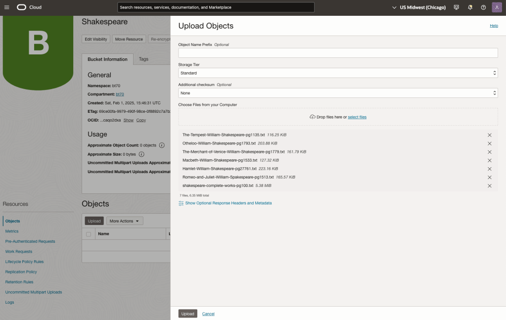
Step-1 Load Files to a Bucket on OCI
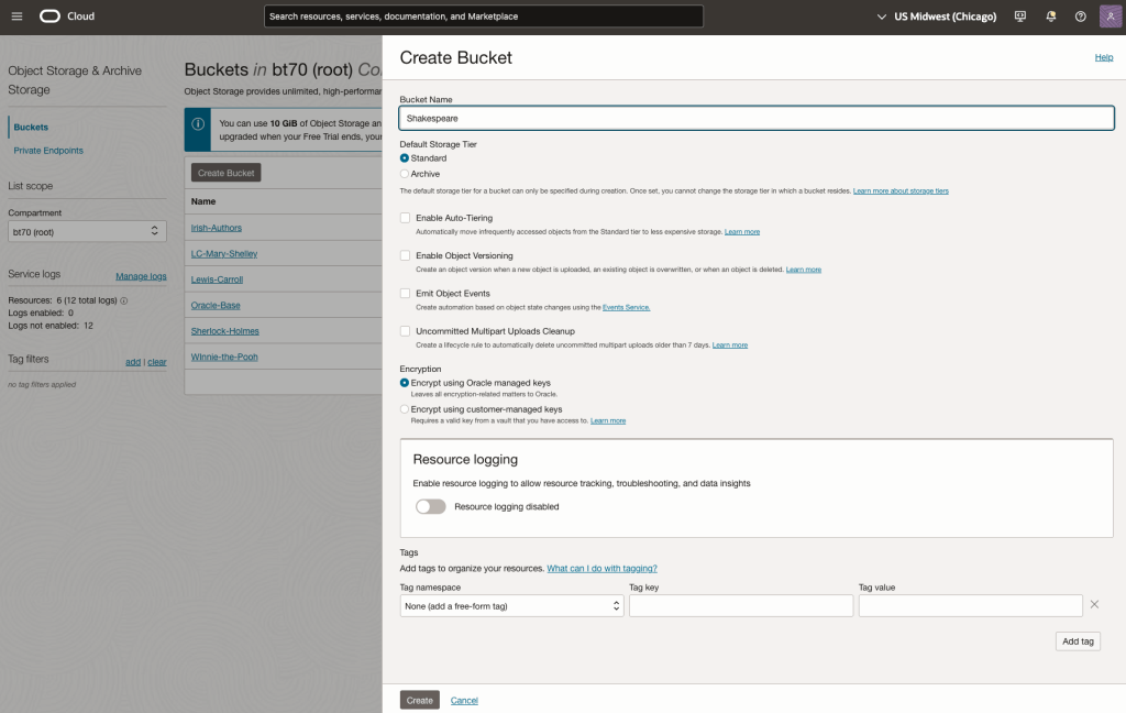
Create a bucket called Shakespeare.
Load the files from your computer into the Bucket. These files were obtained from the Gutenberg Project site.
Step-2 Define a Data Source (documents you want to use) & Create a Knowledge Base
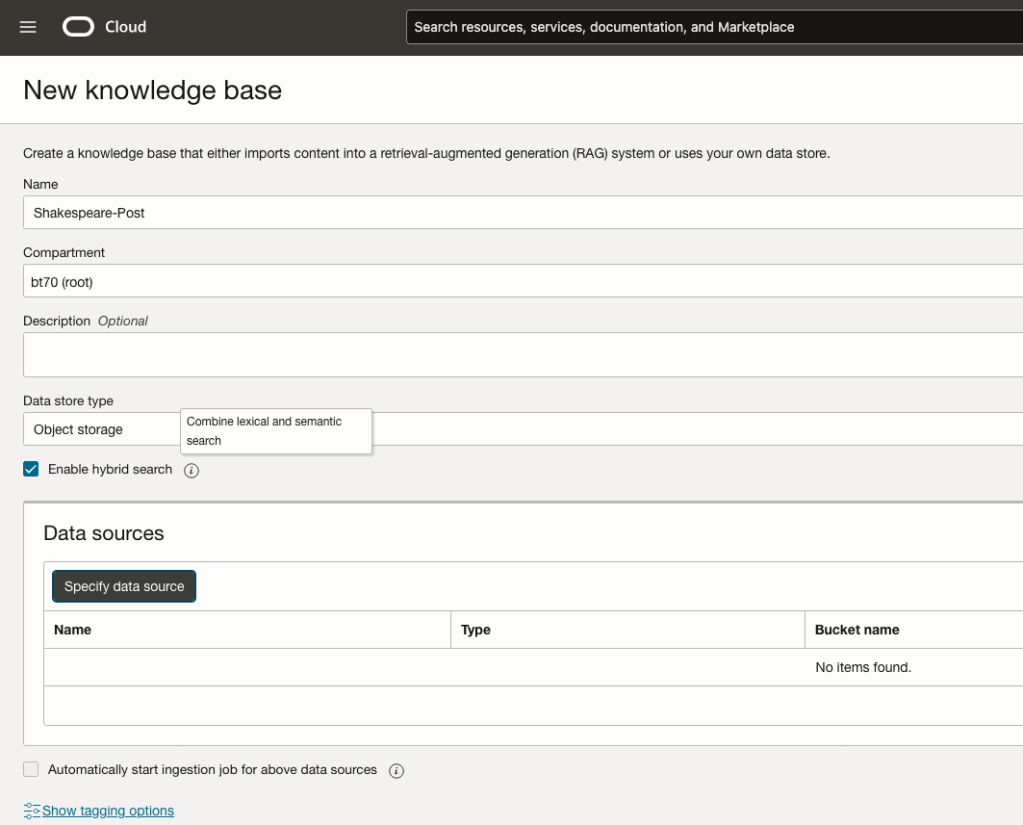
Click on Create Knowledge Base and give it a name ‘Shakespeare’.
Check the ‘Enable Hybrid Search’. checkbox. This will enable both lexical and semantic search. [this is Important]
Click on ‘Specify Data Source’
Select the Bucket from the drop-down list (Shakespeare bucket).
Check the ‘Enable multi-modal parsing’ checkbox.
Select the files to use or check the ‘Select all in bucket’
Click Create.

The Knowledge Base will be created. The files in the bucket will be parsed, and structured for search by the AI Agent. This step can take a few minutes as it needs to process all the files. This depends on the number of files to process, their format and the size of the contents in each file.
Step-3 Create Agent
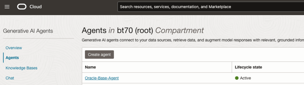
Go back to the main Gen AI menu and select Agent and then Create Agent.
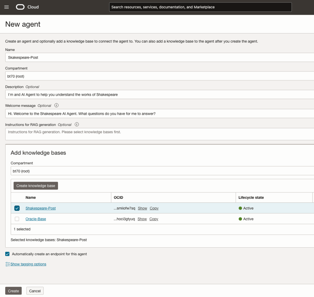
You can enter the following details:
- Name of the Agent
- Some descriptive information
- A Welcome message for people using the Agent
- Select the Knowledge Base from the list.
The checkbox for creating Endpoints should be checked.
Click Create.
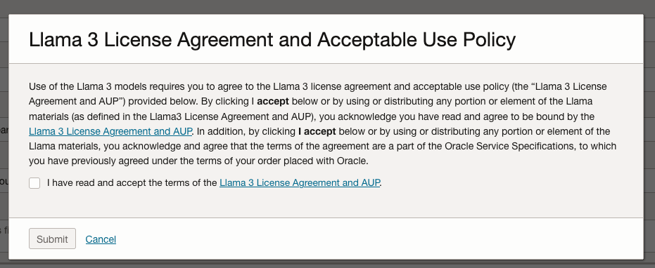
A pop-up window will appear asking you to agree to the Llama 3 License. Check this checkbox and click Submit.
After the agent has been created, check the status of the endpoints. These generally take a little longer to create, and you need these before you can test the Agent using the Chatbot.
Step-4 Test using Chatbot
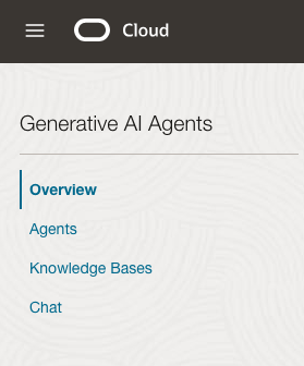
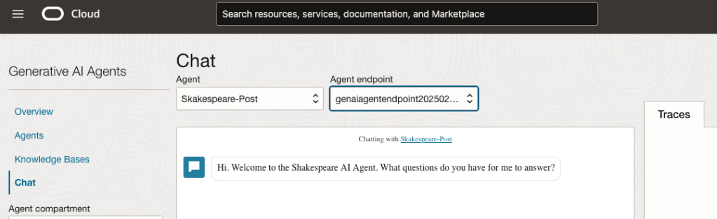
After verifying the endpoints have been created, you can open a Chatbot by clicking on ‘Chat’ from the menu on the left-hand side of the screen.
Select the name of the ‘Agent’ from the drop-down list e.g. Shakespeare-Post.
Select an end-point for the Agent.
After these have been selected you will see the ‘Welcome’ message. This was defined when creating the Agent.
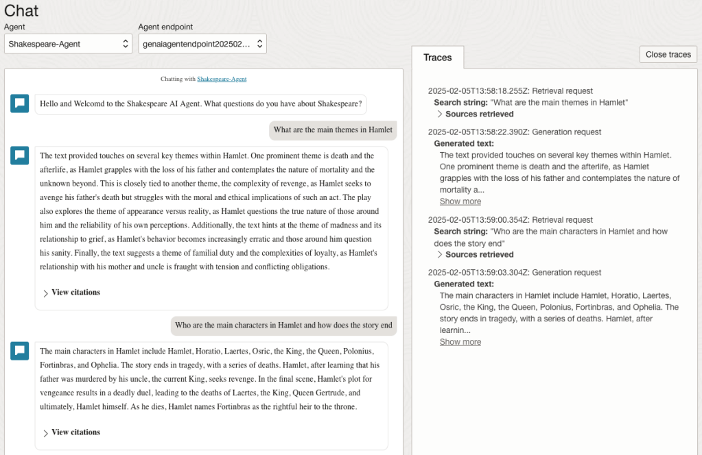
Here are a couple of examples of querying the works by Shakespeare.
In addition to giving a response to the questions, the Chatbot also lists the sections of the underlying documents and passages from those documents used to form the response/answer.
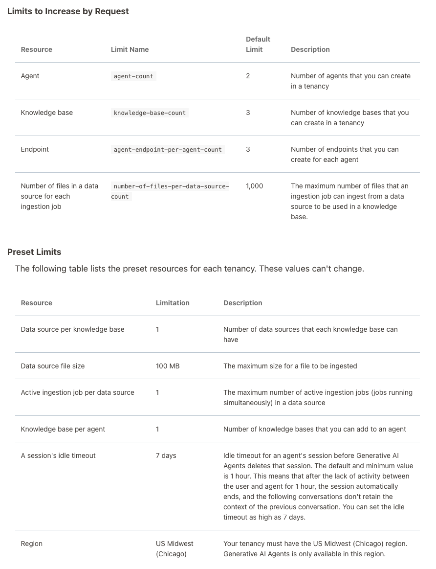
When creating Gen AI Agents, you need to be careful of two things. The first is the Cloud Region. Gen AI Agents are only available in certain Cloud Regions. If they aren’t available in your Region, you’ll need to request access to one of those or setup a new OCI account based in one of those regions. The second thing is the Resource Limits. At the time of writing this post, the following was allowed. Check out the documentation for more details. You might need to request that these limits be increased.
I’ll have another post showing how you can run the Chatbot on your computer or VM as a webpage.
Select AI – OpenAI changes
A few weeks ago I wrote a few blog posts about using SelectAI. These illustrated integrating and using Cohere and OpenAI with SQL commands in your Oracle Cloud Database. See these links below.
- SelectAI – the beginning of a journey
- SelectAI – Doing something useful
- SelectAI – Can metadata help
- SelectAI – the APEX version
With the constantly changing world of APIs, has impacted the steps I outlined in those posts, particularly if you are using the OpenAI APIs. Two things have changed since writing those posts a few weeks ago. The first is with creating the OpenAI API keys. When creating a new key you need to define a project. For now, just select ‘Default Project’. This is a minor change, but it has caused some confusion for those following my steps in this blog post. I’ve updated that post to reflect the current setup in defining a new key in OpenAI. This is a minor change, oh and remember to put a few dollars into your OpenAI account for your key to work. I put an initial $10 into my account and a few minutes later API key for me from my Oracle (OCI) Database.
The second change is related to how the OpenAI API is called from Oracle (OCI) Databases. The API is now expecting a model name. From talking to the Oracle PMs, they will be implementing a fix in their Cloud Databases where the default model will be ‘gpt-3.5-turbo’, but in the meantime, you have to explicitly define the model when creating your OpenAI profile.
BEGIN
   --DBMS_CLOUD_AI.drop_profile(profile_name => 'COHERE_AI');

   DBMS_CLOUD_AI.create_profile(
      profile_name => 'COHERE_AI',
      attributes => '{"provider": "cohere",
                      "credential_name": "COHERE_CRED",
                      "object_list": [{"owner": "SH", "name": "customers"},
                                      {"owner": "SH", "name": "sales"},
                                      {"owner": "SH", "name": "products"},
                                      {"owner": "SH", "name": "countries"},
                                      {"owner": "SH", "name": "channels"},
                                      {"owner": "SH", "name": "promotions"},
                                      {"owner": "SH", "name": "times"}],
                      "model":"gpt-3.5-turbo"
       }');
END;
Other model names you could use include gpt-4 or gpt-4o.
SelectAI – the APEX version
I’ve written a few blog posts about the new Select AI feature on the Oracle Database. In this post, I’ll explore how to use this within APEX, because you have to do things in a different way.
The previous posts on Select AI are:
- SelectAI – the beginning of a journey
- SelectAI – Doing something useful
- SelectAI – Can metadata help
- SelectAI – the APEX version
We have seen in my previous posts how the PL/SQL package called DBMS_CLOUD_AI was used to create a profile. This profile provided details of what provided to use (Cohere or OpenAI in my examples), and what metadata (schemas, tables, etc) to send to the LLM. When you look at the DBMS_CLOUD_AI PL/SQL package it only contains seven functions (at time of writing this post). Most of these functions are for managing the profile, such as creating, deleting, enabling, disabling and setting the profile attributes. But there is one other important function called GENERATE. This function can be used to send your request to the LLM.
Why is the DBMS_CLOUD_AI.GENERATE function needed? We have seen in my previous posts using Select AI using common SQL tools such as SQL Developer, SQLcl and SQL Developer extension for VSCode. When using these tools we need to enable the SQL session to use Select AI by setting the profile. When using APEX or creating your own PL/SQL functions, etc. You’ll still need to set the profile, using
EXEC DBMS_CLOUD_AI.set_profile('OPEN_AI');We can now use the DBMS_CLOUD_AI.GENERATE function to run our equivalent Select AI queries. We can use this to run most of the options for Select AI including showsql, narrate and chat. It’s important to note here that runsql is not supported. This was the default action when using Select AI. Instead, you obtain the necessary SQL using showsql, and you can then execute the returned SQL yourself in your PL/SQL code.
Here are a few examples from my previous posts:
SELECT DBMS_CLOUD_AI.GENERATE(prompt       => 'what customer is the largest by sales',
                              profile_name => 'OPEN_AI',
                              action       => 'showsql')
FROM dual;

SELECT DBMS_CLOUD_AI.GENERATE(prompt       => 'how many customers in San Francisco are married',
                              profile_name => 'OPEN_AI',
                              action       => 'narrate')
FROM dual;

SELECT DBMS_CLOUD_AI.GENERATE(prompt       => 'who is the president of ireland',
                              profile_name => 'OPEN_AI',
                              action       => 'chat')
FROM dual;
If using Oracle 23c or higher you no longer need to include the FROM DUAL;
SelectAI – Can metadata help
Continuing with the exploration of Select AI, in this post I’ll look at how metadata can help. In my previous posts on Select AI, I’ve walked through examples of exploring the data in the SH schema and how you can use some of the conversational features. These really give a lot of potential for developing some useful features in your apps.
Many of you might have encountered schemas here either the table names and/or column names didn’t make sense. Maybe their names looked like some weird code or something, and you had to look up a document, often referred to as a data dictionary, to decode the actual meaning. In some instances, these schemas cannot be touched and in others, minor changes are allowed. In these later cases, we can look at adding some metadata to the tables to give meaning to these esoteric names.
For the following example, I’ve taken the simple EMP-DEPT tables and renamed the table and column names to something very generic. You’ll see I’ve added comments to explain the Tables and for each of the Columns. These comments should correspond to the original EMP-DEPT tables.
CREATE TABLE TABLE1(
c1  NUMBER(2) not null primary key,
c2  VARCHAR2(50) not null,
c3  VARCHAR2(50) not null);

COMMENT ON TABLE table1 IS 'Department table. Contains details of each Department including Department Number, Department Name and Location for the Department';

COMMENT ON COLUMN table1.c1 IS 'Department Number. Primary Key. Unique. Used to join to other tables';
COMMENT ON COLUMN table1.c1 IS 'Department Name. Name of department. Description of function';
COMMENT ON COLUMN table1.c3 IS 'Department Location. City where the department is located';

-- create the EMP table as  TABLE2
CREATE TABLE TABLE2(
c1  NUMBER(4) not null primary key,
c2  VARCHAR2(50) not null,
c3  VARCHAR2(50) not null,
c4  NUMBER(4),
c5  DATE,
c6  NUMBER(10,2),
c7  NUMBER(10,2),
c8  NUMBER(2) not null);

COMMENT ON TABLE table2 IS 'Employee table. Contains details of each Employee. Employees';

COMMENT ON COLUMN table2.c1 IS 'Employee Number. Primary Key. Unique. How each employee is idendifed';
COMMENT ON COLUMN table2.c1 IS 'Employee Name. Name of each Employee';
COMMENT ON COLUMN table2.c3 IS 'Employee Job Title. Job Role. Current Position';
COMMENT ON COLUMN table2.c4 IS 'Manager for Employee. Manager Responsible. Who the Employee reports to';
COMMENT ON COLUMN table2.c5 IS 'Hire Date. Date the employee started in role. Commencement Date';
COMMENT ON COLUMN table2.c6 IS 'Salary. How much the employee is paid each month. Dollars';
COMMENT ON COLUMN table2.c7 IS 'Commission. How much the employee can earn each month in commission. This is extra on top of salary';
COMMENT ON COLUMN table2.c8 IS 'Department Number. Foreign Key. Join to Department Table';

insert into table1 values (10,'Accounting','New York');
insert into table1 values (20,'Research','Dallas');
insert into table1 values (30,'Sales','Chicago');
insert into table1 values (40,'Operations','Boston');

alter session set nls_date_format = 'YY/MM/DD';

insert into table2 values (7369,'SMITH','CLERK',7902,'93/6/13',800,0.00,20);
insert into table2 values (7499,'ALLEN','SALESMAN',7698,'98/8/15',1600,300,30);
insert into table2 values (7521,'WARD','SALESMAN',7698,'96/3/26',1250,500,30);
insert into table2 values (7566,'JONES','MANAGER',7839,'95/10/31',2975,null,20);
insert into table2 values (7698,'BLAKE','MANAGER',7839,'92/6/11',2850,null,30);
insert into table2 values (7782,'CLARK','MANAGER',7839,'93/5/14',2450,null,10);
insert into table2 values (7788,'SCOTT','ANALYST',7566,'96/3/5',3000,null,20);
insert into table2 values (7839,'KING','PRESIDENT',null,'90/6/9',5000,0,10);
insert into table2 values (7844,'TURNER','SALESMAN',7698,'95/6/4',1500,0,30);
insert into table2 values (7876,'ADAMS','CLERK',7788,'99/6/4',1100,null,20);
insert into table2 values (7900,'JAMES','CLERK',7698,'00/6/23',950,null,30);
insert into table2 values (7934,'MILLER','CLERK',7782,'00/1/21',1300,null,10);
insert into table2 values (7902,'FORD','ANALYST',7566,'97/12/5',3000,null,20);
insert into table2 values (7654,'MARTIN','SALESMAN',7698,'98/12/5',1250,1400,30);
Can Select AI be used to query this data? The simple answer is ‘ish’. Yes, Select AI can query this data but some care is needed on how you phrase the questions, and some care is needed to refine the metadata descriptions given in the table and column Comments.
To ensure these metadata Comments are exposed to the LLMs, we need to include the following line in our Profile
"comments":"true",Using the same Profile setup I used for OpenAI, we need to include the tables and the (above) comments:true command. See below in bold
BEGIN
  DBMS_CLOUD_AI.drop_profile(profile_name => 'OPEN_AI');
  DBMS_CLOUD_AI.create_profile(
      profile_name => 'OPEN_AI',
      attributes => '{"provider": "openai",
                      "credential_name": "OPENAI_CRED",
                      "comments":"true",
                      "object_list": [{"owner": "BRENDAN", "name": "TABLE1"},
                                     {"owner": "BRENDAN", "name": "TABLE2"}],
            "model":"gpt-3.5-turbo"
       }');
END;
After we set the profile for our session, we can now write some statements to explore the data.
Warning: if you don’t include “comments”:”true”, you’ll get no results being returned.
Here are a few of what I wrote.
select ai what departments do we have;
select AI showsql what departments do we have;

select ai count departments;
select AI showsql count department;

select ai how many employees;
select ai how many employees work in department 30;
select ai count unique job titles;
select ai list cities where departments are located;
select ai how many employees work in New York;
select ai how many people work in each city;
select ai where are the departments located;
select ai what is the average salary for each department;
Check out the other posts about Select AI.
SelectAI – Doing something useful
In a previous post, I introduced Select AI and gave examples of how to do some simple things. These included asking it using some natural language questions, to query some data in the Database. That post used both Cohere and OpenAI to process the requests. There were mixed results and some gave a different, somewhat disappointing, outcome. But with using OpenAI the overall outcome was a bit more positive. To build upon the previous post, this post will explore some of the additional features of Select AI, which can give more options for incorporating Select AI into your applications/solutions.
Select AI has five parameters, as shown in the table below. In the previous post, the examples focused on using the first parameter. Although those examples didn’t include the parameter name ‘runsql‘. It is the default parameter and can be excluded from the Select AI statement. Although there were mixed results from using this default parameter ‘runsql’, it is the other parameters that make things a little bit more interesting and gives you opportunities to include these in your applications. In particular, the ‘narrate‘ and ‘explainsql‘ parameters and to a lesser extent the ‘chat‘ parameter. Although for the ‘chat’ parameter there are perhaps slightly easier and more efficient ways of doing this.
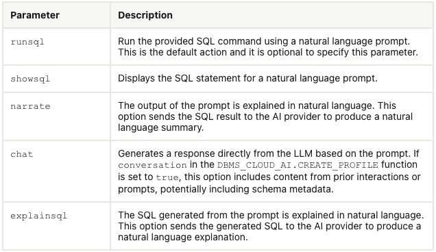
Let’s start by looking at the ‘chat‘ parameter. This allows you to ‘chat’ LLM just like you would with ChatGPT and other similar. A useful parameter to set in the CREATE_PROFILE is to set the conversation to TRUE, as that can give more useful results as the conversation develops.
BEGIN
  DBMS_CLOUD_AI.drop_profile(profile_name => 'OPEN_AI');
  DBMS_CLOUD_AI.create_profile(
      profile_name => 'OPEN_AI',
      attributes => '{"provider": "openai",
                      "credential_name": "OPENAI_CRED",
                      "object_list": [{"owner": "SH", "name": "customers"},
                                      {"owner": "SH", "name": "sales"},
                                      {"owner": "SH", "name": "products"},
                                      {"owner": "SH", "name": "countries"},
                                      {"owner": "SH", "name": "channels"},
                                      {"owner": "SH", "name": "promotions"},
                                      {"owner": "SH", "name": "times"}],
        "conversation": "true",        "model":"gpt-3.5-turbo"       }');
END;
There are a few statements I’ve used.
select AI chat who is the president of ireland;
select AI chat what role does NAMA have in ireland;
select AI chat what are the annual revenues of Oracle;
select AI chat who is the largest cloud computing provider;
select AI chat can you rank the cloud providers by income over the last 5 years;
select AI chat what are the benefits of using Oracle Cloud;
As you’d expect the results can be ‘kind of correct’, with varying levels of information given. I’ve tried these using Cohere and OpenAI, and their responses illustrate the need for careful testing and evaluation of the various LLMs to see which one suits your needs.
In my previous post, I gave some examples of using Select AI to query data in the Database based on a natural language request. Select AI takes that request and sends it, along with details of the objects listed in the create_profile, to the LLM. The LLM then sends back the SQL statement, which is then executed in the Database and the results are displayed. But what if you want to see the SQL generated by the LLM. To see the SQL you can use the ‘showsql‘ parameter. Here are a couple of examples:
SQL> select AI showsql how many customers in San Francisco are married;

RESPONSE
_____________________________________________________________________________SELECT COUNT(*) AS total_married_customers
FROM SH.CUSTOMERS c
WHERE c.CUST_CITY = 'San Francisco'
AND c.CUST_MARITAL_STATUS = 'Married'

SQL> select AI what customer is the largest by sales;

   CUST_ID CUST_FIRST_NAME    CUST_LAST_NAME       TOTAL_SALES
__________ __________________ _________________ ______________
     11407 Dora               Rice                   103412.66


SQL> select AI showsql what customer is the largest by sales;

RESPONSE
_____________________________________________________________________________SELECT C.CUST_ID, C.CUST_FIRST_NAME, C.CUST_LAST_NAME, SUM(S.AMOUNT_SOLD) AS TOTAL_SALES
FROM SH.CUSTOMERS C
JOIN SH.SALES S ON C.CUST_ID = S.CUST_ID
GROUP BY C.CUST_ID, C.CUST_FIRST_NAME, C.CUST_LAST_NAME
ORDER BY TOTAL_SALES DESC
FETCH FIRST 1 ROW ONLY
The examples above that illustrate the ‘showsql‘ is kind of interesting. Careful consideration of how and where to use this is needed.
Where things get a little bit more interesting with the ‘narrate‘ parameter, which attempts to narrate or explain the output from the query. There are many use cases where this can be used to supplement existing dashboards, etc. The following are examples of using ‘narrate‘ for the same two queries used above.
SQL> select AI narrate how many customers in San Francisco are married;

RESPONSE
________________________________________________________________
The total number of married customers in San Francisco is 18.


SQL> select AI narrate what customer is the largest by sales;

RESPONSE
_____________________________________________________________________________To find the customer with the largest sales, you can use the following SQL query:

```sql
SELECT c.CUST_FIRST_NAME || ' ' || c.CUST_LAST_NAME AS CUSTOMER_NAME, SUM(s.AMOUNT_SOLD) AS TOTAL_SALES
FROM "SH"."CUSTOMERS" c
JOIN "SH"."SALES" s ON c.CUST_ID = s.CUST_ID
GROUP BY c.CUST_FIRST_NAME, c.CUST_LAST_NAME
ORDER BY TOTAL_SALES DESC
FETCH FIRST 1 ROW ONLY;
```

This query joins the "CUSTOMERS" and "SALES" tables on the customer ID and calculates the total sales for each customer. It then sorts the results in descending order of total sales and fetches only the first row, which represents the customer with the largest sales.

The result will be in the following format:

| CUSTOMER_NAME | TOTAL_SALES |
|---------------|-------------|
| Tess Drumm    | 161882.79   |

In this example, the customer with the largest sales is "Tess Drumm" with a total sales amount of 161,882.79.
Looking at the outputs from using the ‘narrate‘ parameter, we can see the level of detail given and see the potential of including this kind of information in our applications, dashboards, etc. But to use this output some additional filtering and subsetting will need to be performed.
The final parameter is called ‘explainsql‘. While it may not be as useful as the ‘narrate‘ parameter, it does have some potential uses. The ‘explainsql‘ attempts to explain in natural language what a SQL query is attempting to do, based on a natural language statement. Again using the same two examples, we get the following.
SQL> select AI explainsql what customer is the largest by sales;

RESPONSE
_____________________________________________________________________________SELECT C.CUST_ID, C.CUST_FIRST_NAME, C.CUST_LAST_NAME, SUM(S.AMOUNT_SOLD) AS TOTAL_SALES
FROM SH.CUSTOMERS C
JOIN SH.SALES S ON C.CUST_ID = S.CUST_ID
GROUP BY C.CUST_ID, C.CUST_FIRST_NAME, C.CUST_LAST_NAME
ORDER BY TOTAL_SALES DESC
FETCH FIRST 1 ROW ONLY;

Explanation:
- The query selects the customer ID, first name, last name, and the sum of the amount sold from the CUSTOMERS and SALES tables.
- The CUSTOMERS and SALES tables are joined on the CUST_ID column.
- The results are grouped by customer ID, first name, and last name.
- The results are then ordered in descending order by the total sales.
- The FETCH FIRST 1 ROW ONLY clause is used to retrieve only the top row with the highest total sales.

SQL> select AI explainsql how many customers in San Francisco are married;

RESPONSE
_____________________________________________________________________________
SELECT COUNT(*) AS total_married_customers
FROM SH.CUSTOMERS c
WHERE c.CUST_CITY = 'San Francisco'
AND c.CUST_MARITAL_STATUS = 'Married';

This query selects the count of customers who are married and live in San Francisco. The table alias "c" is used for the CUSTOMERS table. The condition "c.CUST_CITY = 'San Francisco'" filters the customers who live in San Francisco, and the condition "c.CUST_MARITAL_STATUS = 'Married'" filters the customers who are married. The result is the total number of married customers in San Francisco.
Check out the other posts about Select AI.

You must be logged in to post a comment.