
Migrating Python ML Models to other languages
I’ve mentioned in a previous blog post about experiencing some performance issues with using Python ML in production. We needed something quicker and the possible languages we considered were C, C++, Java and Go Lang.
But the data science team used R and Python, with just a few more people using Python than R on the team.
One option was to rewrite everything into the language used in production. As you can imagine no-one wanted to do that and there was no way of ensure a bug free solution and one that gave similar results to the R and Python models. The other option was to look for some code to convert the models from one language to another.
The R users was well versed in using PMML. Predictive Model Markup Language (PMML) has been around a long time and well known and used by certain groups of data scientists who have been around a while. It is also widely supported by many analytics vendors, and provides an inter-change format to allow predictive models to be described and exchanged. For newer people, they hadn’t heard of it. PMML is an XML based interchange specification.
But with PMML there are some limitation. Not with the specification but how it is implemented by the various vendors that support it. PMML supports the exchange of the model pipeline including the data transformations as well as the model specification. Most vendors only support some elements of this and maybe just a couple of models. And there-in lies the problem. How can a ML pipeline be migrated from, as Python, to some other language and/or tool. There are limitations.
If you do want to explore PMML with Python check out the sklearn2pmml package and is also available on PyPl. This package allows you to export the ML pipeline and the model specification. As with most other implementations of PMML there are some parts of the PMML specification not implement, but it is better than post of the other implementation out there.
An alternative is to look at code translations options. With these we want something that will take our ML pipeline and convert it to another programming language like C++, JAVA, Go, etc. There aren’t too many solutions available to do this. One such solution we’ve explored over the past couple of weeks is called m2cgen.
m2cgen (Model 2 Code Generator) is a lightweight library which provides an easy way to transpile trained statistical models into a native code (Python, C, Java, Go). You can supply M2cgen with a range of models (linear, SVM, tree, random forest, or boosting, etc) and the tool will output code in the chosen language that will represent the trained model. The code generated will generated into native code without dependencies. Other packages or libraries are not dependent or required in the translated language. For example here is an example Decision Tree translated into a number of different languages.
C
#include <string.h>
void score(double * input, double * output) {
    double var0[3];
    if ((input[2]) <= (2.6)) {
        memcpy(var0, (double[]){1.0, 0.0, 0.0}, 3 * sizeof(double));
    } else {
        if ((input[2]) <= (4.8500004)) {
            if ((input[3]) <= (1.6500001)) {
                memcpy(var0, (double[]){0.0, 1.0, 0.0}, 3 * sizeof(double));
            } else {
                memcpy(var0, (double[]){0.0, 0.3333333333333333, 0.6666666666666666}, 3 * sizeof(double));
            }
        } else {
            if ((input[3]) <= (1.75)) {
                memcpy(var0, (double[]){0.0, 0.42857142857142855, 0.5714285714285714}, 3 * sizeof(double));
            } else {
                memcpy(var0, (double[]){0.0, 0.0, 1.0}, 3 * sizeof(double));
            }
        }
    }
    memcpy(output, var0, 3 * sizeof(double));
}
Java
public class Model {

    public static double[] score(double[] input) {
        double[] var0;
        if ((input[2]) <= (2.6)) {
            var0 = new double[] {1.0, 0.0, 0.0};
        } else {
            if ((input[2]) <= (4.8500004)) {
                if ((input[3]) <= (1.6500001)) {
                    var0 = new double[] {0.0, 1.0, 0.0};
                } else {
                    var0 = new double[] {0.0, 0.3333333333333333, 0.6666666666666666};
                }
            } else {
                if ((input[3]) <= (1.75)) {
                    var0 = new double[] {0.0, 0.42857142857142855, 0.5714285714285714};
                } else {
                    var0 = new double[] {0.0, 0.0, 1.0};
                }
            }
        }
        return var0;
    }
}
Go Lang
func score(input []float64) []float64 {
    var var0 []float64
    if (input[2]) <= (2.6) {
        var0 = []float64{1.0, 0.0, 0.0}
    } else {
        if (input[2]) <= (4.8500004) {
            if (input[3]) <= (1.6500001) {
                var0 = []float64{0.0, 1.0, 0.0}
            } else {
                var0 = []float64{0.0, 0.3333333333333333, 0.6666666666666666}
            }
        } else {
            if (input[3]) <= (1.75) {
                var0 = []float64{0.0, 0.42857142857142855, 0.5714285714285714}
            } else {
                var0 = []float64{0.0, 0.0, 1.0}
            }
        }
    }
    return var0
}
Machine Learning with Go Lang
Recently I’ve been having a number of conversations with people in several countries about using Go Lang for machine learning. Most of these people have been struggling with using Python for machine learning and are looking for an alternative that will give them better performance. We have been experimenting with C++ and Go Lang to see what the performance differences are. Most of these are with the execution of the ML code. This is great and everyone is very happy with execution timings, compared to Python.
But, there is a flip side to this. Although we have faster execution timings, there is a down side in that the coding effort is higher, with more lines of code and fewer libraries/packages to support the various ML tasks. But most of these can be easily coded ourselves .
We also looked at some frameworks for converting ML models developed in one language but deployed in production using a different language. More on that in another post.
Overall the extra development work was considered worthwhile for the performance improvement and deployment gains.
Go Lang doesn’t really come with it’s own set of libraries/packages for ML, but those have a number of these that can be used to code up the necessary functions we need for our everyday ML needs.
But are there any Go Lang libraries/packages developed for ML, just like we have for the R Language, etc? The simple answer is YES we have. But the number of these is small in comparison to R and Python. Both of these languages are interpreted languages. But those available for Go are slowly growing.
Here is list of the Go Lang libraries/packages that we examined and evaluated for these projects. Some are available from the Go Lang website/wiki and others are available on Github.
- Anna – Artificial Neural Network Aspiration, aims to be self-learning and self-improving software.
- bayesian – A naive bayes classifier.
- Dialex – Dialex is a smart pipe that unscrambles text and makes it machine-readable.
- Cloudforest – Ensembles of decision trees
- ctw – Context Tree Weighting and Rissanen-Langdon Arithmetic Coding
- eaopt – An evolutionary optimization library.
- evo – a framework for implementing evolutionary algorithms in Go.
- gobrain – Neural Networks
- Go Learn – Machine Learning for Go
- go-algs/maxflow Maxflow (graph-cuts) energy minimization library.
- go-graph – Graph library for Go/Golang language
- go-galib – Genetic algorithms.
- go-pr – Pattern recognition package in Go lang
- golinear – Linear SVM and logistic regression.
- go-mind – A neural network library built in Go
- go_ml – Linear Regression, Logistic Regression, Neural Networks, Collaborative Filtering, Gaussian Multivariate Distribution.
- go-ml-transpiler – An open source Go transpiler for machine learning models.
- go-mxnet-predictor – Go binding for MXNet c_predict_api to do inference with pre-trained model.
- gorgonia – Neural network primitives library (like Theano or Tensorflow but for Go)
- go-porterstemmer – An efficient native Go clean room implementation of the Porter Stemming algorithm.
- go-pr – Gaussian classifier.
- ntm – Neural Turing Machines implementation
- paicehusk – Go implementation of the Paice/Husk Stemmer
- RF – Random forests implementation in Go
- tfgo – Tensorflow + Go, the gopher way.
Machine Learning Tools and Workbenches
The following is a list of the most commonly used tools and workbenches for machine learning. These are specific to machine learning only. This list does not include any library or frameworks. These are tools and workbenches only. Most offering machine learning tools will include the following features:
- Easy drag and drop capabilities
- Data collection
- Data preparation and cleaning
- Model building
- Data Visualization
- Model Deployment
- Integration with other tools and languages
As more and more organizations implement machine learning, there are two core aims they want to achieve.
- Employee Productivity: Who wants to spend days or weeks writing mundane code to load data, clean data, etc etc etc. No one wants to do this and especially employers don’t want their staff wasting time on this. Instead they are happy to invest in tools and workbenches where a lot or most or all of these mundane tasks are automated for you. You can not concentrate on the important tasks of adding value to your organisation. This saves money, improves employee productivity and employee value.
- Integration with Technical Architecture: Many of these tools and workbenches allow for easy integration with the technical architecture and thereby allowing easy and quick integration of machine learning withe the day to day activities of the organization. This saves money, improves employee productivity and employee value.
SAS
SAS software has been around for every and is the great grand-daddy of analytics and machine learning. They have built a large number of machine learning tools and solutions built upon these for various industries. Their core machine learning tools include SAS Enterprise Miner and SAS Visual Data Mining and Machine Learning.


Microsoft
Microsoft have been improving their Machine Learning offering over the years and most of this is based on the Azure cloud platform with Microsoft Azure Machine Learning Studio and Azure Databricks.


SAP
SAP Leonardo is a cloud based platform for machine learning and supports tight integration with other SAP software.


Oracle
Oracle have a number of machine learning tools and supports for the main machine learning languages. They have built a large number of applications (both cloud and on-premises) with in-built machine learning. Their main tools for machine learning include Oracle Data Miner, Oracle Machine Learning and Oracle Analytics (OAC or DVD versions)


Cloudera
If you work with hadoop and big data then you are probably using Cloudera in some way. Cloudera have hired Hilary Mason as their GM of ML. By taking an “AI factory” approach to turning data into decisions, you can make the process of building, scaling, and deploying enterprise ML and AI solutions automated, repeatable, and predictable—boring even. Cloudera Data Science Workbench is their solution.
IBM
IBM have a number of machine learning tools, one of them being a long standing member of the machine learning community, SPSS Modeler. Other machine learning tools include Watson Studio, IBM Machine Learning for z/OS, and IBM Watson Explorer.


Google have a large number of machine learning solutions including everything from traditional machine learning, into NLP, in Image processing, Video processing, etc. It’s a long list. Many of these come with various APIs to access these features. Most of these revolve around their Google AI Cloud offering. But sticking with the tools and workbenches we have AI Platform Notebooks, Kubeflow, and BigQuery ML.


TensorBoard
TensorBoard is a suite of tools for graphical representation of different aspects and stages of machine learning in TensorFlow.


Amazon
A bit like Goolge, Amazon has a large number of solutions for machine learning and AI, and most of these are available via an API or some cloud service. Amazon SageMaker is their main service.


Looker
Looker connects directly with Google BQML reduces additional complexity for data scientists by eliminating the need to move outputs of predictive models back into the database for use, while also increases the time-to-value for business users, allowing them to operationalize the outputs of predictive metrics to make better decisions every day.


Weka
Weka has been around for a long time and still popular in some research groups. Weka is a collection of machine learning algorithms for data mining tasks. It contains tools for data preparation, classification, regression, clustering, association rules mining, and visualization.


RapidMiner
RapidMiner Studio has been around for a long time and is one of the few more visual workflow tools (that everyone else should be doing).


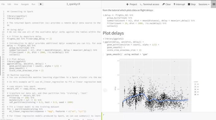
Databricks
From the people who created Spark, we have another notebook solution for your machine learning projects called Databricks Workbench.


KNIME
KNIME Analytics Platform is the open source software for creating data science applications and services.


Dataiku
Dataiki Data Science (DSS) is a collaborative data science software workflow platform enabling data exploration, prototyping and delivery of analytical and machine learning solutions.

")
I’ve not included the tools like R Studio and Notebooks in this list as they don’t really address the aims listed above. But you will notice a lot of the above solutions are really Jupyter Notebooks. Most of these vendors have a long way to go to make the tasks of machine learning boring.
This list does not cover all available tools and workbenches, but it does list the most common one you will come across.
Time Series Forecasting in Oracle – Part 2
This is the second part about time-series data modeling using Oracle. Check out the first part here.
In this post I will take a time-series data set and using the in-database time-series functions model the data, that in turn can be used for predicting future values and trends.
The data set used in these examples is the Rossmann Store Sales data set. It is available on Kaggle and was used in one of their competitions.
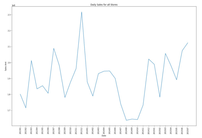
Let’s start by aggregating the data to monthly level. We get.
Data Set-up
Although not strictly necessary, but it can be useful to create a subset of your time-series data to only contain the time related attribute and the attribute containing the data to model. When working with time-series data, the exponential smoothing function expects the time attribute to be of DATE data type. In most cases it does. When it is a DATE, the function will know how to process this and all you need to do is to tell the function the interval.
A view is created to contain the monthly aggregated data.
-- Create input time series
create or replace view demo_ts_data as
select to_date(to_char(sales_date, 'MON-RRRR'),'MON-RRRR') sales_date,
sum(sales_amt) sales_amt
from demo_time_series
group by to_char(sales_date, 'MON-RRRR')
order by 1 asc;
Next a table is needed to contain the various settings for the exponential smoothing function.
CREATE TABLE demo_ts_settings(setting_name VARCHAR2(30),
                              setting_value VARCHAR2(128));
Some care is needed with selecting the parameters and their settings as not all combinations can be used.
Example 1 – Holt-Winters
The first example is to create a Holt-Winters time-series model for hour data set. For this we need to set the parameter to include defining the algorithm name, the specific time-series model to use (exsm_holt), the type/size of interval (monthly) and the number of predictions to make into the future, pass the last data point.
BEGIN
   -- delete previous setttings
   delete from demo_ts_settings;

   -- set ESM as the algorithm
   insert into demo_ts_settings
      values (dbms_data_mining.algo_name,
              dbms_data_mining.algo_exponential_smoothing);

   -- set ESM model to be Holt-Winters
   insert into demo_ts_settings
      values (dbms_data_mining.exsm_model,
              dbms_data_mining.exsm_holt);

   -- set interval to be month
   insert into demo_ts_settings
      values (dbms_data_mining.exsm_interval,
              dbms_data_mining.exsm_interval_month);

   -- set prediction to 4 steps ahead
   insert into demo_ts_settings
      values (dbms_data_mining.exsm_prediction_step,
              '4');

   commit;
END;
Now we can call the function, generate the model and produce the predicted values.
BEGIN
   -- delete the previous model with the same name
   BEGIN
      dbms_data_mining.drop_model('DEMO_TS_MODEL');
   EXCEPTION
      WHEN others THEN null;
   END;

   dbms_data_mining.create_model(model_name => 'DEMO_TS_MODEL',
                                 mining_function => 'TIME_SERIES',
                                 data_table_name => 'DEMO_TS_DATA',
                                 case_id_column_name => 'SALES_DATE',
                                 target_column_name => 'SALES_AMT',
                                 settings_table_name => 'DEMO_TS_SETTINGS');
END;
When the model is created a number of data dictionary views are populated with model details and some addition views are created specific to the model. One such view commences with DM$VP. Views commencing with this contain the predicted values for our time-series model. You need to append the name of the model created, in our example DEMO_TS_MODEL.
-- get predictions
select case_id, value, prediction, lower, upper
from   DM$VPDEMO_TS_MODEL
order by case_id;
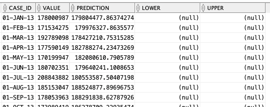
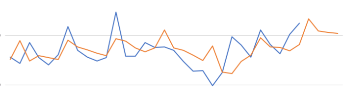
When we plot this data we get.
The blue line contains the original data values and the red line contains the predicted values. The predictions are very similar to those produced using Holt-Winters in Python.

Example 2 – Holt-Winters including Seasonality
The previous example didn’t really include seasonality into the model and predictions. In this example we introduce seasonality to allow the model to pick up any trends in the data based on a defined period.
For this example we will change the model name to HW_ADDSEA, and the season size to 5 units. A data set with a longer time period would illustrate the different seasons better but this gives you an idea.
BEGIN
   -- delete previous setttings
   delete from demo_ts_settings;

   -- select ESM as the algorithm
   insert into demo_ts_settings
   values (dbms_data_mining.algo_name,
           dbms_data_mining.algo_exponential_smoothing);

   -- set ESM model to be Holt-Winters Seasonal Adjusted
   insert into demo_ts_settings
   values (dbms_data_mining.exsm_model,
           dbms_data_mining.exsm_HW_ADDSEA);

   -- set interval to be month
   insert into demo_ts_settings
   values (dbms_data_mining.exsm_interval,
   dbms_data_mining.exsm_interval_month);

  -- set prediction to 4 steps ahead
  insert into demo_ts_settings
  values (dbms_data_mining.exsm_prediction_step,
          '4');

   -- set seasonal cycle to be 5 quarters
   insert into demo_ts_settings
   values (dbms_data_mining.exsm_seasonality,
           '5');

commit;
END;
We need to re-run the creation of the model and produce the predicted values. This code is unchanged from the previous example.
BEGIN
   -- delete the previous model with the same name
   BEGIN
      dbms_data_mining.drop_model('DEMO_TS_MODEL');
   EXCEPTION
      WHEN others THEN null;
   END;

   dbms_data_mining.create_model(model_name => 'DEMO_TS_MODEL',
                                 mining_function => 'TIME_SERIES',
                                 data_table_name => 'DEMO_TS_DATA',
                                 case_id_column_name => 'SALES_DATE',
                                 target_column_name => 'SALES_AMT',
                                 settings_table_name => 'DEMO_TS_SETTINGS');
END;
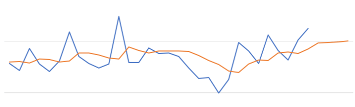
When we re-query the DM$VPDEMO_TS_MODEL we get the new values. When plotted we get.
The blue line contains the original data values and the red line contains the predicted values.
Comparing this chart to the chart from the first example we can see there are some important differences between them. These differences are particularly evident in the second half of the chart, on the right hand side. We get to see there is a clearer dip in the predicted data. This mirrors the real data values better. We also see better predictions as the time line moves to the end.
When performing time-series analysis you really need to spend some time exploring the data, to understand what is happening, visualizing the data, seeing if you can identify any patterns, before moving onto using the different models. Similarly you will need to explore the various time-series models available and the parameters, to see what works for your data and follow the patterns in your data. There is no magic solution in this case.
Data Sets for Analytics
When working with analytics, in whatever flavor, one of the key things you need is some data. But data comes in many different shapes and sizes, but where can you get some useful data, be it transactional, time-series, meta-data, analytical, master, categorical, numeric, regression, clustering, etc.
Many of the popular analytics languages have some data sets built into them. For example the R language comes pre-loaded with data sets and these can be accessed using
data()
but many of the R packages also come with data sets.
Similarly if you are using Python, it comes with some pre-loaded data sets and similarly many of the Python libraries have data sets build into them. For example scikit learn.
from sklearn import datasetsBut where else can you get data sets. There are lots and lots of website available with data sets and the list could be very long. The following is a list of, what I consider, the websites with the best data sets.
Microsoft Research Data Set: https://lnkd.in/eic-WUbQ
Azure Open Data: https://lnkd.in/g6J-zXxb
Amazon Data Set: https://lnkd.in/eRdduaaV
Google DataSet search: https://lnkd.in/egyh_MtM
Pew Research Center posts lots of survey data and other research data: https://lnkd.in/gUVS-8kS
Paperswithcode- the research papers are shared with code repo, often with datasets too: https://lnkd.in/ghpgxEbH
UCI Machine Learning Repository
Awesome Public Datasets Collection
Northern Ireland Public Open Data
Carnegie Mellon University Data Sets
Github List of Public Data Sets
Boston Housing Data Set and from here
ODSC – 25 picks of open data sets
NHS Open Data Sets – including prescriptions issued in England
Time Series Forecasting in Oracle – Part 1
Time-series analysis comprises methods for analyzing time series data in order to extract meaningful statistics and other characteristics of the data. In this blog post I’ll introduce what time-series analysis is, the different types of time-series analysis and introduce how you can do this using SQL and PL/SQL in Oracle Database. I’ll have additional blog posts giving more detailed examples of Oracle functions and how they can be used for different time-series data problems.
Time-series forecasting is the use of a model to predict future values based on previously observed/historical values. It is a form of regression analysis with additions to facilitate trends, seasonal effects and various other combinations.

Time-series forecasting is not an exact science but instead consists of a set of statistical tools and techniques that support human judgment and intuition, and only forms part of a solution. It can be used to automate the monitoring and control of data flows and can then indicate certain trends, alerts, rescheduling, etc., as in most business scenarios it is used for predict some future customer demand and/or products or services needs.
Typical application areas of Time-series forecasting include:
- Operations management: forecast of product sales; demand for services
- Marketing: forecast of sales response to advertisement procedures, new promotions etc.
- Finance & Risk management: forecast returns from investments
- Economics: forecast of major economic variables, e.g. GDP, population growth, unemployment rates, inflation; useful for monetary & fiscal policy; budgeting plans & decisions
- Industrial Process Control: forecasts of the quality characteristics of a production process
- Demography: forecast of population; of demographic events (deaths, births, migration); useful for policy planning
When working with time-series data we are looking for a pattern or trend in the data. What we want to achieve is the find a way to model this pattern/trend and to then project this onto our data and into the future. The graphs in the following image illustrate examples of the different kinds of scenarios we want to model.


Most time-series data sets will have one or more of the following components:
- Seasonal: Regularly occurring, systematic variation in a time series according to the time of year.
- Trend: The tendency of a variable to grow over time, either positively or negatively.
- Cycle: Cyclical patterns in a time series which are generally irregular in depth and duration. Such cycles often correspond to periods of economic expansion or contraction. Also know as the business cycle.
- Irregular: The Unexplained variation in a time series.
When approaching time-series problems you will use a combination of visualizations and time-series forecasting methods to examine the data and to build a suitable model. This is where the skills and experience of the data scientist becomes very important.
Oracle provided a algorithm to support time-series analysis in Oracle 18c. This function is called Exponential Smoothing. This algorithm allows for a number of different types of time-series data and patterns, and provides a wide range of statistical measures to support the analysis and predictions, in a similar way to Holt-Winters.

The first parameter for the Exponential Smoothing function is the name of the model to use. Oracle provides a comprehensive list of models and these are listed in the following table.
Check out my other blog posts on performing time-series analysis using the Exponential Smoothing function in Oracle Database. These will give more detailed examples of how the Oracle time-series functions, using the Exponential Smoothing algorithm, can be used for different time-series data problems. I’ll also look at example of the different configurations.
Python transforming Categorical to Numeric
When preparing data for input to machine learning algorithms you may have to perform certain types of data preparation.
In most enterprise solutions all or most of these tasks are automated for you, but in many languages they aren’t. The enterprise solutions are about ‘automating the boring stuff’ so that you don’t have to worry about it and waste valuable time doing boring, repetitive things.
The following examples illustrates a number of ways to record categorical variables into numeric. There are a number of approaches available, and it is up to you to decide which one might work best for your problem, your data, etc.
Let’s begin by loading the data set to be used in these examples. It is a Video Games reviews data set.
# perform some Statistics on the items in a panda
import pandas as pd
import numpy as np
import matplotlib as plt
videoReview = pd.read_csv('/Users/brendan.tierney/Downloads/Video_Games_Sales_as_at_22_Dec_2016.csv')
videoReview.head(10)

What are the data types of each variable
videoReview.dtypes

We don’t want to work with all the data in these examples. We just want to concentrate on the categorical variables. Let’s us create a subset of the dataframe to contains these.
df = videoReview.select_dtypes(include=['object']).copy()
df.head(10)

Now do a little data clean up by removing NaN (nulls)
df.dropna(inplace=True)
df.isnull().sum()

df.describe()

The above image shows the number of unique values in each of the variables. We will use Platform, Genre and Rating for the variable example below.
Let us chart these variables.
#check the number of passengars for each variable
import seaborn as sb
import matplotlib.pyplot as plt

plt.rcParams['figure.figsize'] = 10, 8

sb.countplot(x='Platform',data=df, palette='hls')

sb.countplot(x='Genre',data=df, palette='hls')

sb.countplot(x='Rating',data=df, palette='hls')

1-One-hot Coding
The first approach is to use the commonly used one-hot coding method. This will take a categorical variable and create a set of new variables corresponding with each distinct value in the variable, and then populate it with a binary value to indicate the original value.
#apply one-hot-coding to all the categorical variables
# and create a new dataframe to store the results

df2 = pd.get_dummies(df)
df2.head(10)

As you can see we now have 8138 variables in the pandas dataframe!
That is a lot and may not be workable for you. You may need to look at some feature reduction methods to reduce the number of variables.
2-Find and Replace
In this example we will simple replace the values with defined values.
Let’s have a look at values in the Ratings variable and their frequencies.
df['Rating'].value_counts()

The last 4 values listed have very small number of occurrences.
We will group these into having one value/category
find_replace = {"Rating" : {"E": 1, "T": 2, "M": 3, "E10+": 4, "EC": 5, "K-A": 5, "RP": 5, "AO": 5}}
df.replace(find_replace, inplace=True)
df.head(10)

Now plot the newly generated rating values and their frequencies.
sb.countplot(x='Rating',data=df, palette='hls')

3 – Label encoding
With this technique where each distinct value in a categorical variable is converted to a number.
In this scenario you don’t get to pick the numeric value assigned to the value. It is system determined.
#let's check the data types again
df.dtypes

Our categorical variables are of ‘object’ data type. We need to convert to a category data type.
In this example ‘Platform’ as it has a large-ish number of values and we want a quick way of converting them we can illustrate this by creating a new variable.
df["Platform_Category"] = df["Platform"].astype('category')
df.dtypes

Now convert this new variable to numeric.
df["Platform_Category"] = df["Platform_Category"].cat.codes
df.head(20)

The number assigned to the Platform_Category variable is based on the alphabetical ordering of the values in the Platform variable. For example,
df.groupby("Platform")["Platform"].count()

4-Using SciKit-Learn transform
SciKit-Learn has a number of functions to help with data encodings. The first one we will look at is the ‘fit_transform’ function.
This will perform a similar task to what we have seen in a previous example
#Let's use the fit_tranforms function to encode the Genre variable
from sklearn.preprocessing import LabelEncoder

le_make = LabelEncoder()
df["Genre_Code"] = le_make.fit_transform(df["Genre"])
df[["Genre", "Genre_Code"]].head(10)

And we can see this comparison when we look at the frequency counts.
df.groupby("Genre_Code")["Genre_Code"].count()

df.head(10)

And now we can drop the Genre variable from the dataframe as it is no longer needed. BUT you will need to have recorded the mapping between the original Genre values and the numeric values for future reference.
df = df.drop('Genre', axis=1)
df.head(10)

5-Using SciKit-Learn LabelEndcoder
SciKit-Learn has a binary label encoder and it can be used in a similar way to the previous example and also similar to the ‘get_dummies’ function.
from sklearn.preprocessing import LabelBinarizer

lb_style = LabelBinarizer()
lb_results = lb_style.fit_transform(df["Rating"])
lb_df = pd.DataFrame(lb_results, columns=lb_style.classes_)
lb_df.head(10)

These can now be joined with the original dataframe or a with a subset of the original dataframe to form a new dataframe consisting of the required variables.
As you can see, from the following, there are several other data pre-processing functions available in SciKit-Learn.

Data Normalization in Oracle Data Mining
Normalization is the process of scaling continuous values down to a specific range, often between zero and one. Normalization transforms each numerical value by subtracting a number, called the shift, and dividing the result by another number called the scale. The normalization techniques include:
- Min-Max Normalization : There is where the normalization is based on the using the minimum value for the shift and the (maximum-minimum) for the scale.
- Scale Normalization : This is where the normalization is based on zero being used for the shift and the value calculated using max[abs(max), abs(min)] being used for the scale
- Z-Score Normalization : This is where the normalization is based on using the mean value for the shift and the standard deviation for the scale.
When using Automatic Data Processing the normalization functions are used. But sometimes you may want to process the data is a more explicit manner. To do so you can use the various normalization function. To use these there is a three stage process. The first stage involves the creation of a table that will contain the normalization transformation data. The second stage applies the normalization procedures to your data source, defines the normalization required and inserts the required transformation data into the table create during the first stage. The third stage involves the defining of a view that applies the normalization transformations to your data source and displays the output via a database view. The following example illustrates how you can normalize the AGE and YRS_RESIDENCE attributes. The input data source will be the view that was created as the output of the previous transformation (MINING_DATA_V_2). This is passed on the original MINING_DATA_BUILD_V data set. The final output from this transformation step and all the other data transformation steps is MINING_DATA_READY_V.
BEGIN
   -- Clean-up : Drop the previously created tables
   BEGIN
      execute immediate 'drop table TRANSFORM_NORMALIZE';
   EXCEPTION
      WHEN others THEN
         null;
   END;

   -- Stage 1 : Create the table for the transformations
   -- Perform normalization for: AGE and YRS_RESIDENCE
   dbms_data_mining_transform.CREATE_NORM_LIN (
      norm_table_name => 'MINING_DATA_NORMALIZE');

   -- Step 2 : Insert the normalization data into the table
   dbms_data_mining_transform.INSERT_NORM_LIN_MINMAX (
      norm_table_name => 'MINING_DATA_NORMALIZE',
      data_table_name => 'MINING_DATA_V_2',
      exclude_list    => DBMS_DATA_MINING_TRANSFORM.COLUMN_LIST (
                         'affinity_card',
                         'bookkeeping_application',
                         'bulk_pack_diskettes',
                         'cust_id',
                         'flat_panel_monitor',
                         'home_theater_package',
                         'os_doc_set_kanji',
                         'printer_supplies',
                         'y_box_games'));

   -- Stage 3 : Create the view with the transformed data
   DBMS_DATA_MINING_TRANSFORM.XFORM_NORM_LIN (
      norm_table_name => 'MINING_DATA_NORMALIZE',
      data_table_name => 'MINING_DATA_V_2',
      xform_view_name => 'MINING_DATA_READY_V');

END;
/
The above example performs normalization based on the Minimum-Maximum values of the variables/columns. The other normalization functions are:
| INSERT_NORM_LIN_SCALE | Inserts linear scale normalization definitions in a transformation definition table. |
| INSERT_NORM_LIN_ZSCORE | Inserts linear zscore normalization definitions in a transformation definition table. |
Hivemall: Feature Scaling based on Min-Max values
Once of the most common tasks when preparing data for data mining and machine learning is to take numerical data and scale it. Most enterprise and advanced tools and languages do this automatically for you, but with lower level languages you need to perform the task. There are a number of approaches to doing this. In this example we will use the Min-Max approach.
With the Min-Max feature scaling approach, we need to find the Minimum and Maximum values of each numerical feature. Then using a scaling function that will re-scale the data to a Zero to One range. The general formula for this is.
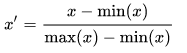
Using the IRIS data set as the data set (and loaded in previous post), the first thing we need to find is the minimum and maximum values for each feature.
select min(features[0]), max(features[0]),
       min(features[1]), max(features[1]),
       min(features[2]), max(features[2]),
       min(features[3]), max(features[3])
from iris_raw;
we get the following results.
4.3 7.9 2.0 4.4 1.0 6.9 0.1 2.5
The format of the results can be a little confusing. What this list gives us is the results for each of the four features.
For feature[0], sepal_length, we have a minimum value of 4.3 and a maximum value of 7.9.
Similarly,
feature[1], sepal_width, min=2.0, max=4.4
feature[2], petal_length, min=1.0, max=6.9
feature[3], petal_width, min=0.1, max=2.5
To use these minimum and maximum values, we need to declare some local session variables to store these.
set hivevar:feature0_min=4.3;
set hivevar:feature0_max=7.9;
set hivevar:feature1_min=2.0;
set hivevar:feature1_max=4.4;
set hivevar:feature2_min=1.0;
set hivevar:feature2_max=6.9;
set hivevar:feature3_min=0.1;
set hivevar:feature3_max=2.5;
After setting those variables we can now write a SQL SELECT and use the add_bias function to perform the calculations.
select rowid, label,
       add_bias(array(
          concat("1:", rescale(features[0],${f0_min},${f0_max})),
          concat("2:", rescale(features[1],${f1_min},${f1_max})),
          concat("3:", rescale(features[2],${f2_min},${f2_max})),
          concat("4:", rescale(features[3],${f3_min},${f3_max})))) as features
from iris_raw;
and we get
> 1 Iris-setosa   ["1:0.22222215","2:0.625","3:0.0677966","4:0.041666664","0:1.0"]
> 2 Iris-setosa   ["1:0.16666664","2:0.41666666","3:0.0677966","4:0.041666664","0:1.0"]
> 3 Iris-setosa   ["1:0.11111101","2:0.5","3:0.05084745","4:0.041666664","0:1.0"]
...
Other feature scaling methods, available in Hivemall, include L1/L2 Normalization and zscore.
OCI – Making DBaaS Accessible using port 1521
When setting up a Database on Oracle Cloud Infrastructure (OCI) for the first time there are a few pre and post steps to complete before you can access the database using a JDBC type of connect, just like what you have in SQL Developer, or using Python or other similar tools and/or languages.
1. Setup Virtual Cloud Network (VCN)
The first step, when starting off with OCI, is to create a Virtual Cloud Network.
Create a VCN and take all the defaults. But change the radio button shown in the following image.
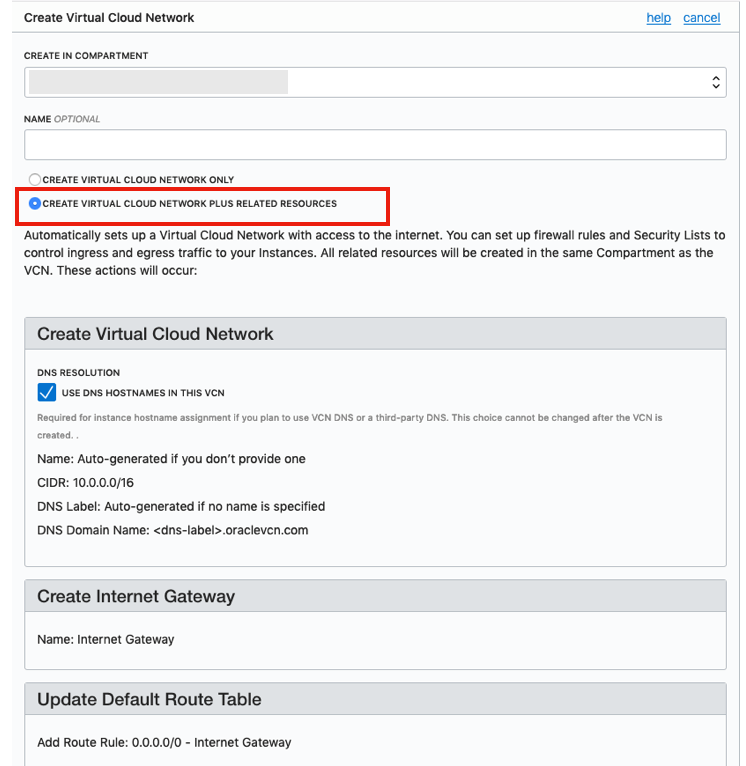
That’s it. We will come back to this later.
2. Create the Oracle Database
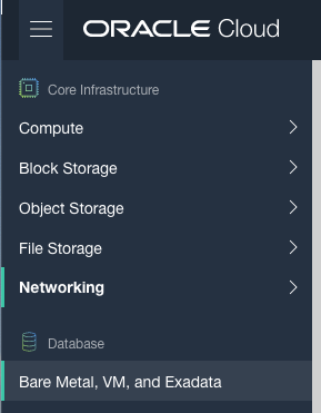
To create the database select ‘Bare Metal, VM and Exadata’ from the menu.
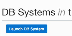
Click on the ‘Launch DB System’ button.
Fill in the details of the Database you want to create and select from the various options from the drop-downs.
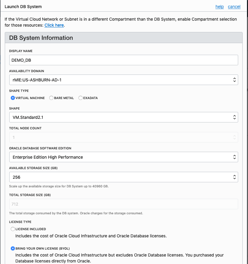
Fill in the details of the VCN you created in the previous set, and give the name of the DB and the Admin password.
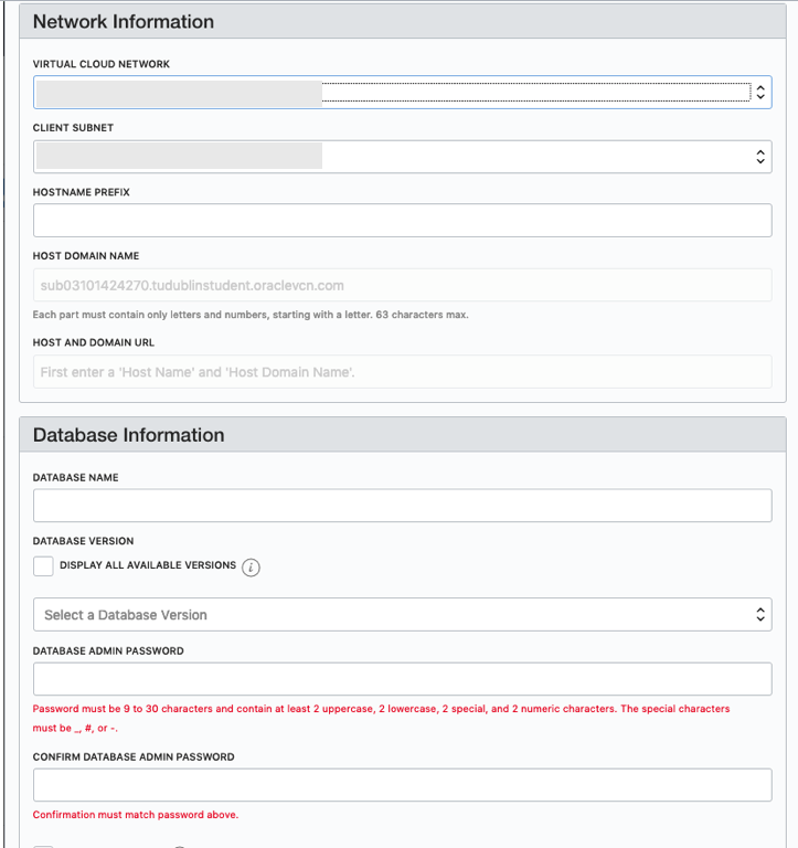
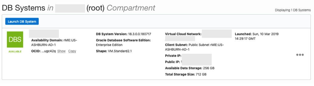
When you are finished everything that is needed, the ‘Launch DB System’ at the bottom of the page will be enabled. After clicking on this botton, the VM will be built and should be ready in a few minutes. When finished you should see something like this.
3. SSH to the Database server
When the DB VM has been created you can now SSH to it. You will need to use the SSH key file used when creating the DB VM. You will need to connect to the opc (operating system user), and from there sudo to the oracle user. For example
ssh -i <ssh file> opc@<public IP address>
The public IP address can be found with the Database VM details
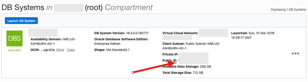
[opc@tudublins1 ~]$ sudo su - oracle
[oracle@tudublins1 ~]$ . oraenv
ORACLE_SID = [cdb1] ?
The Oracle base has been set to /u01/app/oracle
[oracle@tudublins1 ~]$
[oracle@tudublins1 ~]$ sqlplus / as sysdba

SQL*Plus: Release 18.0.0.0.0 - Production on Wed Mar 13 11:28:05 2019
Version 18.3.0.0.0

Copyright (c) 1982, 2018, Oracle. All rights reserved.


Connected to:
Oracle Database 18c Enterprise Edition Release 18.0.0.0.0 - Production
Version 18.3.0.0.0

SQL> alter session set container = pdb1;

Session altered.

SQL> create user demo_user identified by DEMO_user123##;

User created.

SQL> grant create session to demo_user;

Grant succeeded.

SQL>
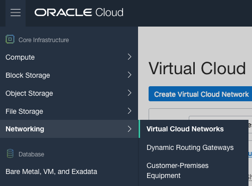
4. Open port 1521
To be able to access this with a Basic connection in SQL Developer and most programming languages, we will need to open port 1521 to allow these tools and languages to connect to the database.
To do this go back to the Virtual Cloud Networks section from the menu.
Click into your VCN, that you created earlier. You should see something like the following.
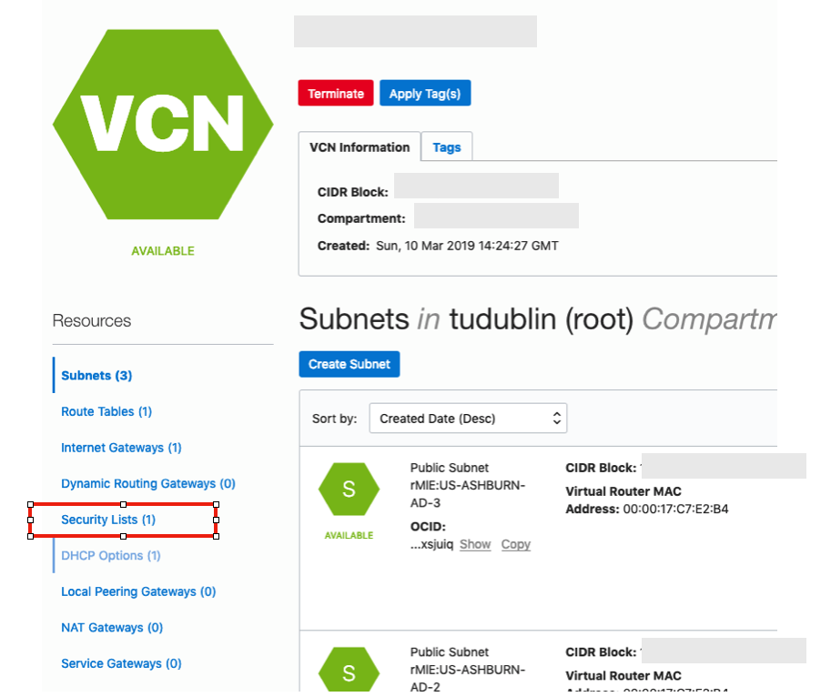
Click on the Security Lists, menu option on the left hand side.
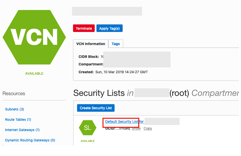 From that screen, click on Default Security List, and then click on the ‘Edit All Rules’ button at the top of the next screen.
Add a new rule to have a ‘Destination Port Range’ set for 1521
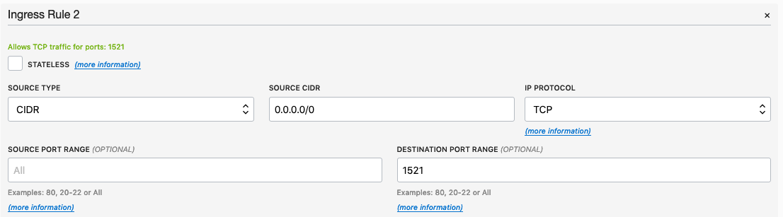
That’s it.
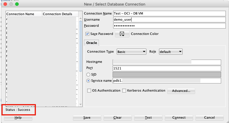
5. Connect to the Database from anywhere
Now you can connect to the OCI Database using a basic SQL Developer Connection.
Moving Average in SQL (and beyond)
A very common analytics technique for financial and other data is to calculate the moving average. This can allow you to see a different type of pattern in your data that may not is evident from examining the original data.
But how can we calculate the moving average in SQL?
Well, there isn’t a function to do it, but we can use the windowing feature of analytical SQL to do so. The following example was created in an Oracle Database but the same SQL (more or less) will work with most other SQL databases.
SELECT month,
       SUM(amount) AS month_amount,
       AVG(SUM(amount)) OVER
          (ORDER BY month ROWS BETWEEN 3 PRECEDING AND CURRENT ROW) AS moving_average
FROM  sales
GROUP BY month
ORDER BY month;
This gives us the following with the moving average calculated based on the current value and the three preceding values, if they exist.
    MONTH MONTH_AMOUNT MOVING_AVERAGE
---------- ------------ --------------
         1     58704.52       58704.52
         2      28289.3       43496.91
         3     20167.83       35720.55
         4      50082.9     39311.1375
         5     17212.66     28938.1725
         6     31128.92     29648.0775
         7     78299.47     44180.9875
         8     42869.64     42377.6725
         9     35299.22     46899.3125
        10     43028.38     49874.1775
        11     26053.46      36812.675
        12     20067.28      31112.085
In some analytic languages and databases, they have included a moving average function. For example using HiveMall on Hive we have.
SELECT moving_avg(x, 3) FROM (SELECT explode(array(1.0,2.0,3.0,4.0,5.0,6.0,7.0)) as x) series;If you are using Python, there is an inbuilt function in Pandas.
rolmean4 = timeseries.rolling(window = 4).mean()
HiveMall: Docker image setup
In a previous blog post I introduced HiveMall as a SQL based machine learning language available for Hadoop and integrated with Hive.
If you have your own Hadoop/Big Data environment, I provided the installation instructions for Hivemall, in that blog post
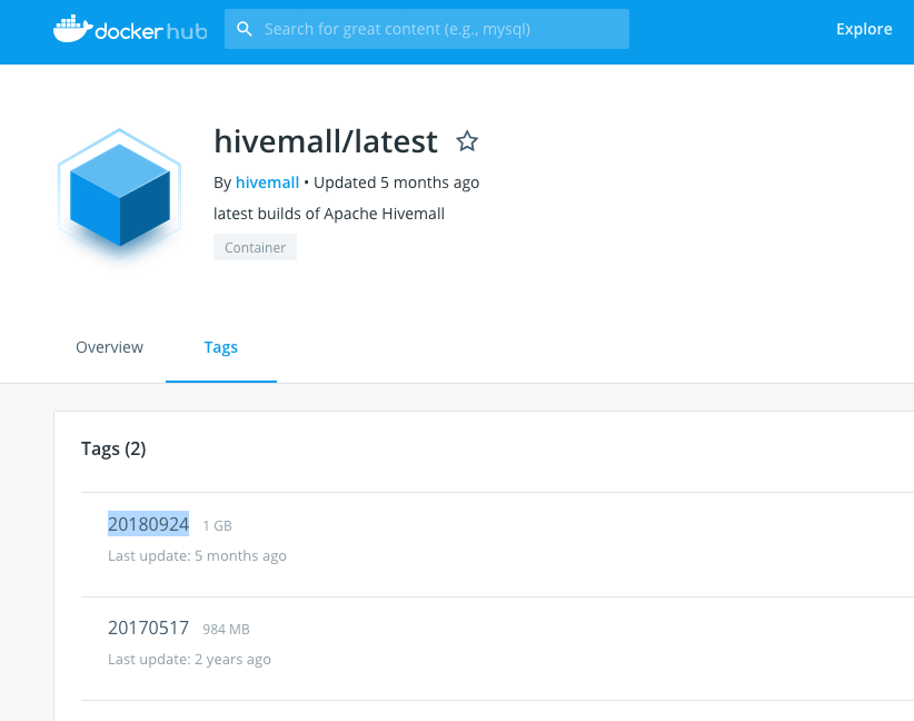
An alternative is to use Docker. There is a HiveMall Docker image available. A little warning before using this image. It isn’t updated with the latest release but seems to get updated twice a year. Although you may not be running the latest version of HiveMall, you will have a working environment that will have almost all the functionality, bar a few minor new features and bug fixes.
To get started, you need to make sure you have Docker running on your machine and you have logged into your account. The docker image is available from Docker Hub. Take note of the version number for the latest version of the docker image. In this example it is 20180924
Open a terminal window and run the following command. This will download and extract all the image files.
docker pull hivemall/latest:20180924

Until everything is completed.

This docker image has HDFS, Yarn and MapReduce installed and running. This will require the exposing of the ports for these services 8088, 50070 and 19888.
To start the HiveMall docker image run
docker run -p 8088:8088 -p 50070:50070 -p 19888:19888 -it hivemall/latest:20180924Consider creating a shell script for this, to make it easier each time you want to run the image.

Now seed Hive with some data. The typical example uses the IRIS data set. Run the following command to do this. This script downloads the IRIS data set, creates a number directories and then creates an external table, in Hive, to point to the IRIS data set.
cd $HOME && ./bin/prepare_iris.sh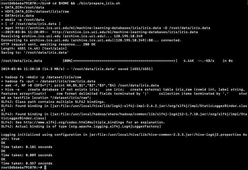
Now open Hive and list the databases.
hive -S
hive> show databases;
OK
default
iris
Time taken: 0.131 seconds, Fetched: 2 row(s)
Connect to the IRIS database and list the tables within it.
hive> use iris;
hive> show tables;
iris_raw
Now query the data (150 records)
hive> select * from iris_raw;
1 Iris-setosa [5.1,3.5,1.4,0.2]
2 Iris-setosa [4.9,3.0,1.4,0.2]
3 Iris-setosa [4.7,3.2,1.3,0.2]
4 Iris-setosa [4.6,3.1,1.5,0.2]
5 Iris-setosa [5.0,3.6,1.4,0.2]
6 Iris-setosa [5.4,3.9,1.7,0.4]
7 Iris-setosa [4.6,3.4,1.4,0.3]
8 Iris-setosa [5.0,3.4,1.5,0.2]
9 Iris-setosa [4.4,2.9,1.4,0.2]
10 Iris-setosa [4.9,3.1,1.5,0.1]
11 Iris-setosa [5.4,3.7,1.5,0.2]
12 Iris-setosa [4.8,3.4,1.6,0.2]
13 Iris-setosa [4.8,3.0,1.4,0.1
...
Find the min and max values for each feature.
hive> select
    > min(features[0]), max(features[0]),
    > min(features[1]), max(features[1]),
    > min(features[2]), max(features[2]),
    > min(features[3]), max(features[3])
    > from
    > iris_raw;

4.3  7.9  2.0  4.4  1.0  6.9  0.1  2.5
You are now up and running with HiveMall on Docker.

You must be logged in to post a comment.