
statistics
Python Data Profiling libraries
One of the most common, and sometimes boring, task when working with datasets is writing some code to profile the data. Most data scientists will have built a set of tools/scripts to help them with this regular and slightly boring task. As with most IT tasks we should be trying to automate what we can, to allow us to spend more time on more important tasks, such as deriving insights and delivering value to the business, instead of repeatedly writing code to produce various statistics about the data and drawing pretty pictures.
I’ve written previously about automating and using some data profiling libraries to help us with this task. There are lots of packages available on pypi.og and on GitHub. Below I give examples of 5 Python Data Profiling libraries, with links to their GitHubs.
This is probably one of the better and more popular Python libraries for exploring data. The aim is to make it as simple as possible using one line of code.
pandas-profilingpackage naming was changed. To continue profiling data useydata-profilinginstead
import pandas_profiling as pp

df2.profile_report()


2. skimpy
Following the line line of code approach skimpy is a light weight tool that provides summary statistics about variables in data frames. They like to thing skimpy is a super-charged version of df.describe(). Skimpy also has some automated data cleaning functions.
from skimpy import skim

skim(df)
3. dataprep
Dataprep has multiple features with the two main features being EDA (Exploratory Data Analysis) and Data Cleaning. For EDA functionality, it is build to scale for larger data sets and provides some interactive charts.
from dataprep.eda import *
from dataprep.datasets import load_dataset
from dataprep.eda import plot, plot_correlation, plot_missing, plot_diff, create_report

df = load_dataset("titanic")
plot(df)

plot_missing(df)
plot_missing(df, "Age")

4. SweetViz
Sweetviz creates high-density visualizations to help kickstart EDA with just two lines of code. Output is a fully self-contained HTML application.
import pandas as pd
import sweetviz as sv

df = pd.read_csv('../input/titanic/train.csv')
report = sweetviz.analyze(df, "Survived")
5. AutoViz
Autoviz works on visualizing the relationship of the data, it can find the most impactful features and plot creative visualization.
from autoviz.AutoViz_Class import AutoViz_Class
AV = AutoViz_Class()

df = AV.AutoViz('titanic_train.csv')
Always try to automate the boring tasks, and using one of these packages is a step towards doing for for any Data Analysts, Data Sciences, Data Engineers, Machine Learning Engineer, AI Engineer, etc.
Measuring Kurtosis of Data in Oracle (21c)
Kurtosis is a new analytics function in Oracle 21c (20c) and is one of a set of commonly used statistical functions used to evaluate data to see and understand the behavior of the data.
[See my previous post where I give examples of the new Skewness functions]
Kurtosis is the measurement of the tails of the data distribution and its comparison with that of normal distribution. The Kurtosis of the normal distribution is said to be 3. To make interpenetrating results easier (a Zero) kurtosis measure for gaussian/normal distribution by subtracting 3 from its value, this is called Excess Kurtosis. Kurtosis can be used to describe the height or the breath of the distributions, when compared to a normal distributions, although this is not theoretically correct, it gives a simpler explanation and visualization of it. The following diagram gives an example of a normal distribution, a plot of Positive Kurtosis and Negative Kurtosis.

Prior to the new Kurtosis SQL functions (KURTOSIS_POP and KURTOSIS_SAMP), you had to calculate the Kurtosis value manually using something like the following SQL. These use the same data and attributes set used for the Skewness examples.
select avg(KV) K_value
from (select power((age - avg(age) over ())/stddev(age) over (), 4) KV
      from cust_data)
union all
select avg(KV) K_value
from (select power((duration - avg(duration) over ())/stddev(duration) over (), 4) KV
      from cust_data);

K_value
------------------------------------------
3.79088571963003808388287765230733611415
23.24420570926391173498028369605428048285
These don’t include the subtraction of 3 to give a zero kurtosis, and these values can be compared to the data distribution charts shown in the Skewness post.
Now with the new Kurtosis functions it simplifies the tasks of getting these values.
SELECT kurtosis_pop(age), kurtosis_samp(age)
FROM bank_additional
union all
SELECT kurtosis_pop(duration), kurtosis_samp(duration)
FROM bank_additional;

KURTOSIS_POP         KURTOSIS_SAMP
------------------   -----------------------------------------
 0.791069803527387    0.79131153115443467194451597661213420763
20.245334438614832   20.24793801497878942299945619307526969226
As you can see the Kurtosis function have the subtraction include.
As with the Skewness functions, the SAMP version works on a sample of the data values and as the number inputs increases, and differences between the POP and SAMP will reduce.
Measuring Skewness of Data in Oracle (21c)
When analyzing data you will look at using a variety of different statistical functions to explore variable data insights.
One of these is the Skewness of the data.
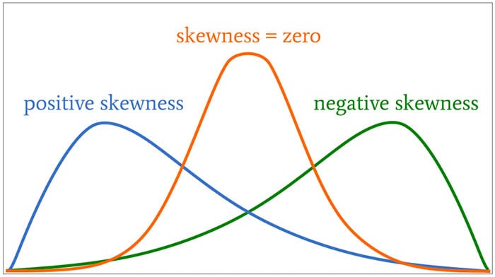
Skewness is a measure of the asymmetry of the probability distribution about its mean. This looks a the tail of the data, with a positive value indicating the tail on the right side of the distribution, and a negative value when the tail is on the left hand side. A zero value indicates the tails on both side balance out, as shown in the following image.
Most SQL dialects support Skewness using with an inbuilt function. But if it doesn’t then you would need to write your own version of the calculation, for example using the following.
SELECT avg(SV) S_value
FROM   (SELECT  power((age – avg(age) over ())/stddev(age) over (), 3) SV
        FROM    cust_data)
Here are charts illustrating the data in my table. These include the distributions for the AGE and DURATION attributes.
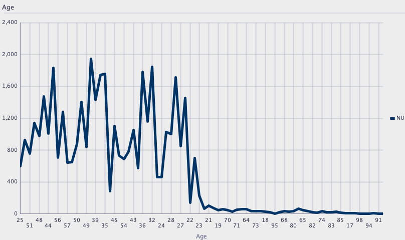

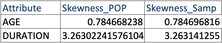
We can see the data is skewed. When we run the above code we get the following values.
Age = 0.78
Duration = 3.26
We can see the skewness of Duration is significantly longer, giving a positive value as the skewness is to the right.
In Oracle 21s we now have new Skewness functions called SKEWNESS_POP and SKEWNESS_SAMP. The POP version of the function considers all records, where as the SAMP function considers a sample of the records. When your data set grows into many millions of records the SKEWNESS_SAMP will give a quicker response as it works with a sample of the data set
Both functions will give similar values but at the number of input records the returned values will returned will converge.
SELECT skewness_pop(age), skewness_samp(age)
FROM cust_data;
SELECT skewness_pop(duration), skewness_samp(duration)
FROM cust_data;
Principal Component Analysis (PCA) in Oracle
Principal Component Analysis (PCA), is a statistical process used for feature or dimensionality reduction in data science and machine learning projects. It summarizes the features of a large data set into a smaller set of features by projecting each data point onto only the first few principal components to obtain lower-dimensional data while preserving as much of the data’s variation as possible. There are lots of resources that goes into the mathematics behind this approach. I’m not going to go into that detail here and a quick internet search will get you what you need.
PCA can be used to discover important features from large data sets (large as in having a large number of features), while preserving as much information as possible.
Oracle has implemented PCA using Sigular Value Decomposition (SVD) on the covariance and correlations between variables, for feature extraction/reduction. PCA is closely related to SVD. PCA computes a set of orthonormal bases (principal components) that are ranked by their corresponding explained variance. The main difference between SVD and PCA is that the PCA projection is not scaled by the singular values. The extracted features are transformed features consisting of linear combinations of the original features.
When machine learning is performed on this reduced set of transformed features, it can completed with less resources and time, while still maintaining accuracy.
Algorithm Name in Oracle using
Mining Model Function = FEATURE_EXTRACTION
Algorithm = ALGO_SINGULAR_VALUE_DECOMP
(Hyper)-Parameters for algorithms
- SVDS_U_MATRIX_OUTPUT : SVDS_U_MATRIX_ENABLE or SVDS_U_MATRIX_DISABLE
- SVDS_SCORING_MODE : SVDS_SCORING_SVD or SVDS_SCORING_PCA
- SVDS_SOLVER : possible values include SVDS_SOLVER_TSSVD, SVDS_SOLVER_TSEIGEN, SVDS_SOLVER_SSVD, SVDS_SOLVER_STEIGEN
- SVDS_TOLERANCE : range of 0…1
- SVDS_RANDOM_SEED : range of 0…4294967296 (!)
- SVDS_OVER_SAMPLING : range of 1…5000
- SVDS_POWER_ITERATIONS : Default value 2, with possible range of 0…20
Let’s work through an example using the MINING_DATA_BUILD_V data set that comes with Oracle Data Miner.
First step is to define the parameter settings for the algorithm. No data preparation is needed as the algorithm takes care of this. This means you can disable the Automatic Data Preparation (ADP).
-- create the parameter table
CREATE TABLE svd_settings (
setting_name VARCHAR2(30),
setting_value VARCHAR2(4000));

-- define the settings for SVD algorithm
BEGIN
   INSERT INTO svd_settings (setting_name, setting_value)
   VALUES (dbms_data_mining.algo_name, dbms_data_mining.algo_singular_value_decomp);

   -- turn OFF ADP
   INSERT INTO svd_settings (setting_name, setting_value)
   VALUES (dbms_data_mining.prep_auto, dbms_data_mining.prep_auto_off);

   -- set PCA scoring mode
   INSERT INTO svd_settings (setting_name, setting_value)
   VALUES (dbms_data_mining.svds_scoring_mode, dbms_data_mining.svds_scoring_pca);

   INSERT INTO svd_settings (setting_name, setting_value)
   VALUES (dbms_data_mining.prep_shift_2dnum, dbms_data_mining.prep_shift_mean);

   INSERT INTO svd_settings (setting_name, setting_value)
   VALUES (dbms_data_mining.prep_scale_2dnum, dbms_data_mining.prep_scale_stddev);
END;
/
You are now ready to create the model.
BEGIN
   DBMS_DATA_MINING.CREATE_MODEL(
      model_name          => 'SVD_MODEL',
      mining_function     => dbms_data_mining.feature_extraction,
      data_table_name     => 'mining_data_build_v',
      case_id_column_name => 'CUST_ID',
      settings_table_name => 'svd_settings');
END;
When created you can use the mining model data dictionary views to explore the model and to explore the specifics of the model and the various MxN matrix created using the model specific views. These include:
- DM$VESVD_Model : Singular Value Decomposition S Matrix
- DM$VGSVD_Model : Global Name-Value Pairs
- DM$VNSVD_Model : Normalization and Missing Value Handling
- DM$VSSVD_Model : Computed Settings
- DM$VUSVD_Model : Singular Value Decomposition U Matrix
- DM$VVSVD_Model : Singular Value Decomposition V Matrix
- DM$VWSVD_Model : Model Build Alerts
Where the S, V and U matrix contain:
- U matrix : consists of a set of ‘left’ orthonormal bases
- S matrix : is a diagonal matrix
- V matrix : consists of set of ‘right’ orthonormal bases
These can be explored using the following
-- S matrix
select feature_id, VALUE, variance, pct_cum_variance
from DM$VESVD_MODEL;

-- V matrix
select feature_id, attribute_name, value
from DM$VVSVD_MODEL
order by feature_id, attribute_name;

-- U matrix
select feature_id, attribute_name, value
from DM$VVSVD_MODEL
order by feature_id, attribute_name;
To determine the projections to be used for visualizations we can use the FEATURE_VALUES function.
select FEATURE_VALUE(svd_sh_sample, 1 USING *) proj1,
       FEATURE_VALUE(svd_sh_sample, 2 USING *) proj2
from   mining_data_build_v
where  cust_id <= 101510
order by 1, 2;
Other algorithms available in Oracle for feature extraction and reduction include:
- Non-Negative Matrix Factorization (NMF)
- Explicit Semantic Analysis (ESA)
- Minimum Description Length (MDL) – this is really feature selection rather than feature extraction
Managing imbalanced Data Sets with SMOTE in Python
When working with data sets for machine learning, lots of these data sets and examples we see have approximately the same number of case records for each of the possible predicted values. In this kind of scenario we are trying to perform some kind of classification, where the machine learning model looks to build a model based on the input data set against a target variable. It is this target variable that contains the value to be predicted. In most cases this target variable (or feature) will contain binary values or equivalent in categorical form such as Yes and No, or A and B, etc or may contain a small number of other possible values (e.g. A, B, C, D).
For the classification algorithm to perform optimally and be able to predict the possible value for a new case record, it will need to see enough case records for each of the possible values. What this means, it would be good to have approximately the same number of records for each value (there are many ways to overcome this and these are outside the score of this post). But most data sets, and those that you will encounter in real life work scenarios, are never balanced, as in having a 50-50 split. What we typically encounter might be a 90-10, 98-2, etc type of split. These data sets are said to be imbalanced.

The image above gives examples of two approaches for creating a balanced data set. The first is under-sampling. This involves reducing the class that contains the majority of the case records and reducing it to match the number of case records in the minor class. The problems with this include, the resulting data set is too small to be meaningful, the case records removed could contain important records and scenarios that the model will need to know about.
The second example is creating a balanced data set by increasing the number of records in the minority class. There are a few approaches to creating this. The first approach is to create duplicate records, from the minor class, until such time as the number of case records are approximately the same for each class. This is the simplest approach. The second approach is to create synthetic records that are statistically equivalent of the original data set. A commonly technique used for this is called SMOTE, Synthetic Minority Oversampling Technique. SMOTE uses a nearest neighbors algorithm to generate new and synthetic data we can use for training our model. But one of the issues with SMOTE is that it will not create sample records outside the bounds of the original data set. As you can image this would be very difficult to do.
The following examples will illustrate how to perform Under-Sampling and Over-Sampling (duplication and using SMOTE) in Python using functions from Pandas, Imbalanced-Learn and Sci-Kit Learn libraries.
NOTE: The Imbalanced-Learn library (e.g. SMOTE)requires the data to be in numeric format, as it statistical calculations are performed on these. The python function get_dummies was used as a quick and simple to generate the numeric values. Although this is perhaps not the best method to use in a real project. With the other sampling functions can process data sets with a sting and numeric.
Data Set: Is the Portuaguese Banking data set and is available on the UCI Data Set Repository, and many other sites. Here are some basics with that data set.
import warnings

import pandas as pd
import numpy as np
import matplotlib.pyplot as plt
get_ipython().magic('matplotlib inline')

bank_file = ".../bank-additional-full.csv"

# import dataset
df = pd.read_csv(bank_file, sep=';',)

# get basic details of df (num records, num features)
df.shape
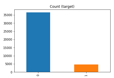
df['y'].value_counts() # dataset is imbalanced with majority of class label as "no".
no     36548
yes     4640
Name: y, dtype: int64
#print bar chart
df.y.value_counts().plot(kind='bar', title='Count (target)');
Example 1a – Down/Under sampling the majority class y=1 (using random sampling)
count_class_0, count_class_1 = df.y.value_counts()

# Divide by class
df_class_0 = df[df['y'] == 0] #majority class
df_class_1 = df[df['y'] == 1] #minority class

# Sample Majority class (y=0, to have same number of records as minority calls (y=1)
df_class_0_under = df_class_0.sample(count_class_1)
# join the dataframes containing y=1 and y=0
df_test_under = pd.concat([df_class_0_under, df_class_1])

print('Random under-sampling:')
print(df_test_under.y.value_counts())
print("Num records = ", df_test_under.shape[0])

df_test_under.y.value_counts().plot(kind='bar', title='Count (target)');

Example 1b – Down/Under sampling the majority class y=1 using imblearn
from imblearn.under_sampling import RandomUnderSampler

X = df_new.drop('y', axis=1)
Y = df_new['y']

rus = RandomUnderSampler(random_state=42, replacement=True)
X_rus, Y_rus = rus.fit_resample(X, Y)

df_rus = pd.concat([pd.DataFrame(X_rus), pd.DataFrame(Y_rus, columns=['y'])], axis=1)

print('imblearn over-sampling:')
print(df_rus.y.value_counts())
print("Num records = ", df_rus.shape[0])

df_rus.y.value_counts().plot(kind='bar', title='Count (target)');
[same results as Example 1a]
Example 1c – Down/Under sampling the majority class y=1 using Sci-Kit Learn
from sklearn.utils import resample

print("Original Data distribution")
print(df['y'].value_counts())

# Down Sample Majority class
down_sample = resample(df[df['y']==0],
replace = True, # sample with replacement
n_samples = df[df['y']==1].shape[0], # to match minority class
random_state=42) # reproducible results

# Combine majority class with upsampled minority class
train_downsample = pd.concat([df[df['y']==1], down_sample])

# Display new class counts
print('Sci-Kit Learn : resample : Down Sampled data set')
print(train_downsample['y'].value_counts())
print("Num records = ", train_downsample.shape[0])
train_downsample.y.value_counts().plot(kind='bar', title='Count (target)');
[same results as Example 1a]
Example 2 a – Over sampling the minority call y=0 (using random sampling)
df_class_1_over = df_class_1.sample(count_class_0, replace=True)
df_test_over = pd.concat([df_class_0, df_class_1_over], axis=0)

print('Random over-sampling:')
print(df_test_over.y.value_counts())

df_test_over.y.value_counts().plot(kind='bar', title='Count (target)');
Random over-sampling:
1    36548
0    36548
Name: y, dtype: int64

Example 2b – Over sampling the minority call y=0 using SMOTE
from imblearn.over_sampling import SMOTE

print(df_new.y.value_counts())
X = df_new.drop('y', axis=1)
Y = df_new['y']

sm = SMOTE(random_state=42)
X_res, Y_res = sm.fit_resample(X, Y)

df_smote_over = pd.concat([pd.DataFrame(X_res), pd.DataFrame(Y_res, columns=['y'])], axis=1)

print('SMOTE over-sampling:')
print(df_smote_over.y.value_counts())

df_smote_over.y.value_counts().plot(kind='bar', title='Count (target)');
[same results as Example 2a]
Example 2c – Over sampling the minority call y=0 using Sci-Kit Learn
from sklearn.utils import resample

print("Original Data distribution")
print(df['y'].value_counts())

# Upsample minority class
train_positive_upsample = resample(df[df['y']==1],
replace = True, # sample with replacement
n_samples = train_zero.shape[0], # to match majority class
random_state=42) # reproducible results

# Combine majority class with upsampled minority class
train_upsample = pd.concat([train_negative, train_positive_upsample])

# Display new class counts
print('Sci-Kit Learn : resample : Up Sampled data set')
print(train_upsample['y'].value_counts())
train_upsample.y.value_counts().plot(kind='bar', title='Count (target)');
[same results as Example 2a]
Time Series Forecasting in Oracle – Part 1
Time-series analysis comprises methods for analyzing time series data in order to extract meaningful statistics and other characteristics of the data. In this blog post I’ll introduce what time-series analysis is, the different types of time-series analysis and introduce how you can do this using SQL and PL/SQL in Oracle Database. I’ll have additional blog posts giving more detailed examples of Oracle functions and how they can be used for different time-series data problems.
Time-series forecasting is the use of a model to predict future values based on previously observed/historical values. It is a form of regression analysis with additions to facilitate trends, seasonal effects and various other combinations.
Time-series forecasting is not an exact science but instead consists of a set of statistical tools and techniques that support human judgment and intuition, and only forms part of a solution. It can be used to automate the monitoring and control of data flows and can then indicate certain trends, alerts, rescheduling, etc., as in most business scenarios it is used for predict some future customer demand and/or products or services needs.
Typical application areas of Time-series forecasting include:
- Operations management: forecast of product sales; demand for services
- Marketing: forecast of sales response to advertisement procedures, new promotions etc.
- Finance & Risk management: forecast returns from investments
- Economics: forecast of major economic variables, e.g. GDP, population growth, unemployment rates, inflation; useful for monetary & fiscal policy; budgeting plans & decisions
- Industrial Process Control: forecasts of the quality characteristics of a production process
- Demography: forecast of population; of demographic events (deaths, births, migration); useful for policy planning
When working with time-series data we are looking for a pattern or trend in the data. What we want to achieve is the find a way to model this pattern/trend and to then project this onto our data and into the future. The graphs in the following image illustrate examples of the different kinds of scenarios we want to model.


Most time-series data sets will have one or more of the following components:
- Seasonal: Regularly occurring, systematic variation in a time series according to the time of year.
- Trend: The tendency of a variable to grow over time, either positively or negatively.
- Cycle: Cyclical patterns in a time series which are generally irregular in depth and duration. Such cycles often correspond to periods of economic expansion or contraction. Also know as the business cycle.
- Irregular: The Unexplained variation in a time series.
When approaching time-series problems you will use a combination of visualizations and time-series forecasting methods to examine the data and to build a suitable model. This is where the skills and experience of the data scientist becomes very important.
Oracle provided a algorithm to support time-series analysis in Oracle 18c. This function is called Exponential Smoothing. This algorithm allows for a number of different types of time-series data and patterns, and provides a wide range of statistical measures to support the analysis and predictions, in a similar way to Holt-Winters.

The first parameter for the Exponential Smoothing function is the name of the model to use. Oracle provides a comprehensive list of models and these are listed in the following table.
Check out my other blog posts on performing time-series analysis using the Exponential Smoothing function in Oracle Database. These will give more detailed examples of how the Oracle time-series functions, using the Exponential Smoothing algorithm, can be used for different time-series data problems. I’ll also look at example of the different configurations.

You must be logged in to post a comment.