
Changing PDB/CDB spfile parameters
When working with a Oracle database hosted on the Oracle cloud (not an Autonomous DB), I recently had the need to change/increase the number of processes for the database. After a bit of researching it looked liked I just had to make the change to the SPFILE and that would be it.
I needed to change/increase the PROCESSES parameter for the CDB and the PDB. Following the multitude of advice on the internet, I ssh into the DB server, found the SPFILE and changed it.
I bounced the DB and when I connected to the PDB, I found the number for PROCESSES was still the same as the old/original value. Nothing had changed.
By default the initialization parameter for the PDB inherit the values from the parameters for the CDB. But this didn’t seem to be the case.
After a bit more research, I needed to set this parameter for the CDB and the PDB. But no luck finding a parameter file for the PDB. It turns out the parameters for the PDB are set at the metadata level, and I needed to change the parameter there.
What I had to do was to change the value when connected to it using SQL*Plus, SQL Dev etc. So, How did I change the parameter value.
Using SQL Developer as my tool, I connected as SYSDBA to my PDB. Then ran,
alter session set container = cdb$root
Now change the parameter value.
alter system set processes = 1200 scope=both
I then bounced the database, logged back into my PDB as system and checked the parameter values. It worked. This was such a simple solution and it worked for me, but there was way too many articles, blog posts, etc out there that didn’t work. Something I’ll need to investigate later is, did I need to connect to the CDB? could I have just run the second command only? I need to setup a different/test DB and see.
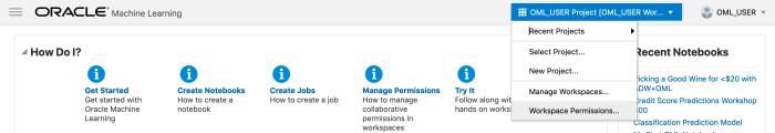
OML Workspace Permissions
When working with Oracle Machine Learning (OML) you are creating notebooks which focus on a particular data exploration and possibly some machine learning. Despite it’s name, OML is used extensively for data discovery and data exploration.
One of the aims of using OML, or notebooks in general, is that these can be easily shared with other people either within the same team or beyond. Something to consider when sharing notebooks is what you are allowing other people do with your notebook. Without any permissions you are allowing people to inspect, run and modify the notebooks. This can be a problem because those people you are sharing with may or may not be allowed to make modification. Some people should be able to just view the notebook, and others should be able to more advanced tasks.
With OML Notebooks there are four primary types of people who can access Notebooks and these can have different privileges. These are defined as
- Developer : Can create new notebooks withing a project and workspace but cannot create a workspace or a project. Can create and run a notebook as a scheduled job.
- Viewer : They can just view projects, Workspaces and notebooks. They are not allowed to create or run anything.
- Manager : can create new notebooks and projects. But only view Workspaces. Additionally they can schedule notebook jobs.
- Administrators : Administrators of the OML environment do not have any edit capabilities on notebooks. But they can view them.

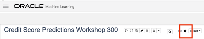
OML Notebooks Interpreter Bindings
When using Oracle Machine Learning notebooks, you can export and import these between different projects and different environments (from ADW to ATP).
But something to watch out for when you import a notebook into your ADW or ATP environment is to reset the Interpreter Bindings.
When you create a new OML Notebook and build it up, the various Interpreter Bindings are automatically set or turned on. But for Imported OML Notebooks they are not turned on.
I’m assuming this will be fixed at some future point.
If you import an OML Notebook and turn on the Interpreter Bindings you may find the code in your notebook cells running very slowly
To turn on these binding, click on the options icon as indicated by the red box in the following image.
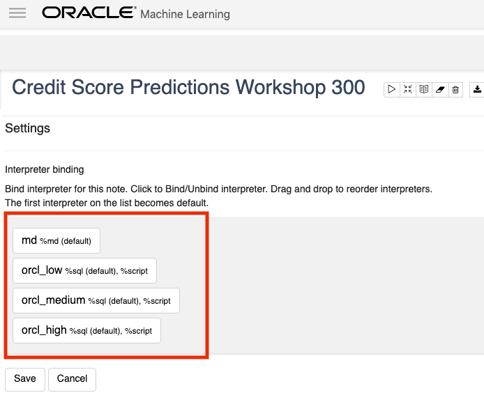
You will get something like the following being displayed. None of the bindings are highlighted.
To enable the Interpreter Bindings just click on each of these boxes. When you do this each one will be highlighted and will turn a blue color.
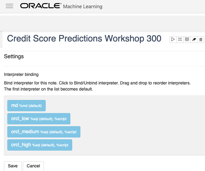
All done! You can now run your OML Notebooks without any problems or delays.
ADW – Loading data using Object Storage
There are a number of different ways to load data into your Autonomous Data Warehouse (ADW) environment. I’ll have posts about these alternatives.
In this blog post I’ll go through the steps needed to load data using Object Storage. This might appear to have a large-ish number of steps, but once you have gone through it and have some of the parts already setup and configuration from your first time, then the second and subsequent times will be easier.
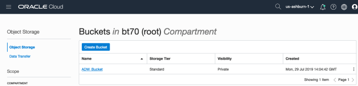
After logging into your Oracle Cloud dashboard, select Object Storage from the side menu.

Then click on the Create Bucket button.

Enter a name for the Object Storage bucket, take the defaults for the for the rest, and click on the Create Bucket button at the bottom. In my example, I’ve called the bucket ‘ADW_Bucket’.

Click on the name of the bucket in the list.
And then click Upload Objects button.

In the Upload Objects window, browse for the file(s) you want to upload.


Then click on the Upload Objects button on the Upload Objects window. After a few moments you will see a message saying the file(s) have been uploaded. Click on the Close window.
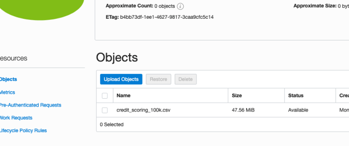
Click into the Object details and take a note/copy of the URL Path. You will need this later
To load data from the Oracle Cloud Infrastructure(OCI) Object Storage you will need an OCI user with the appropriate privileges to read data (or upload) data to the Object Store. The communication between the database and the object store relies on the Swift protocol and the OCI user Auth Token. Go back to the menu in the upper left and select users.


Then click on the user name to view the details. This is probably your OCI username.
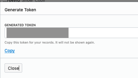
On the left hand side of the page click Auth Tokens, and then click on Generate Token button. Give a name for the token e.g ADW_TOKEN, and then generate token.
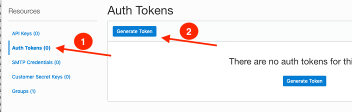
Save the generated token to use later.
Open SQL Developer and setup a connection to your OML User/schema. When connected the next steps is to authenticate with the Object storage using your OCI username and the Auth Token, generated above.
BEGIN
  DBMS_CLOUD.CREATE_CREDENTIAL(
    credential_name => 'ADW_TOKEN',
    username => '<your cloud username>',
    password => '<generated auth token>'
  );
END;
If successful you should get the following message. If not then you probably entered something incorrectly. Go back and review the previous steps
PL/SQL procedure successfully completed.
Next, create a table to store the data you want to import. For my table the create table is the following. [It is one of the sample data sets for OML, and I’ve made the create table statement compact to save space in this post]
create table credit_scoring_100k
( customer_id number(38,0), age number(4,0), income number(38,0), marital_status varchar2(26 byte),
number_of_liables number(3,0), wealth varchar2(4000 byte), education_level varchar2(26 byte),
tenure number(4,0), loan_type varchar2(26 byte), loan_amount number(38,0),
loan_length number(5,0), gender varchar2(26 byte), region varchar2(26 byte),
current_address_duration number(5,0), residental_status varchar2(26 byte),
number_of_prior_loans number(3,0), number_of_current_accounts number(3,0),
number_of_saving_accounts number(3,0), occupation varchar2(26 byte),
has_checking_account varchar2(26 byte), credit_history varchar2(26 byte),
present_employment_since varchar2(26 byte), fixed_income_rate number(4,1),
debtor_guarantors varchar2(26 byte), has_own_phone_no varchar2(26 byte),
has_same_phone_no_since number(4,0), is_foreign_worker varchar2(26 byte),
number_of_open_accounts number(3,0), number_of_closed_accounts number(3,0),
number_of_inactive_accounts number(3,0), number_of_inquiries number(3,0),
highest_credit_card_limit number(7,0), credit_card_utilization_rate number(4,1),
delinquency_status varchar2(26 byte), new_bankruptcy varchar2(26 byte),
number_of_collections number(3,0), max_cc_spent_amount number(7,0),
max_cc_spent_amount_prev number(7,0), has_collateral varchar2(26 byte),
family_size number(3,0), city_size varchar2(26 byte), fathers_job varchar2(26 byte),
mothers_job varchar2(26 byte), most_spending_type varchar2(26 byte),
second_most_spending_type varchar2(26 byte), third_most_spending_type varchar2(26 byte),
school_friends_percentage number(3,1), job_friends_percentage number(3,1),
number_of_protestor_likes number(4,0), no_of_protestor_comments number(3,0),
no_of_linkedin_contacts number(5,0), average_job_changing_period number(4,0),
no_of_debtors_on_fb number(3,0), no_of_recruiters_on_linkedin number(4,0),
no_of_total_endorsements number(4,0), no_of_followers_on_twitter number(5,0),
mode_job_of_contacts varchar2(26 byte), average_no_of_retweets number(4,0),
facebook_influence_score number(3,1), percentage_phd_on_linkedin number(4,0),
percentage_masters number(4,0), percentage_ug number(4,0),
percentage_high_school number(4,0), percentage_other number(4,0),
is_posted_sth_within_a_month varchar2(26 byte), most_popular_post_category varchar2(26 byte),
interest_rate number(4,1), earnings number(4,1), unemployment_index number(5,1),
production_index number(6,1), housing_index number(7,2), consumer_confidence_index number(4,2),
inflation_rate number(5,2), customer_value_segment varchar2(26 byte),
customer_dmg_segment varchar2(26 byte), customer_lifetime_value number(8,0),
churn_rate_of_cc1 number(4,1), churn_rate_of_cc2 number(4,1),
churn_rate_of_ccn number(5,2), churn_rate_of_account_no1 number(4,1),
churn_rate__of_account_no2 number(4,1), churn_rate_of_account_non number(4,2),
health_score number(3,0), customer_depth number(3,0),
lifecycle_stage number(38,0), credit_score_bin varchar2(100 byte));
After creating the table, you are ready to import the data from Object storage. To do this you will need to use the DBMS_COULD PL/SQL package.
begin
   dbms_cloud.copy_data(
   table_name =>'credit_scoring_100k',
   credential_name =>'ADW_TOKEN',
   file_uri_list => '<url of file in your Object Store bucket, see comment earlier in post>',
   format => json_object('ignoremissingcolumns' value 'true', 'removequotes' value 'true', 'dateformat' value 'YYYY-MM-DD HH24:MI:SS', 'blankasnull' value 'true', 'delimiter' value ',', 'skipheaders' value '1')
);
end;
All done.
You can now query the data and use with Oracle Machine Learning, etc.
[I said at the top of the post there are other methods available. More on this in other posts]
Oracle ADW how to load new OML notebooks
Oracle Autonomous Database (ADW) has been out a while now and have had several, behind the scenes, improvements and new/additional features added.
If you have used the Oracle Machine Learning (OML) component of ADW you will have seen the various sample OML Notebooks that come pre-loaded. These are easy to open, use and to try out the various OML features.
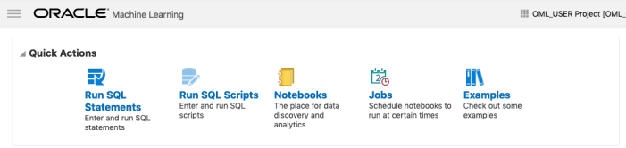
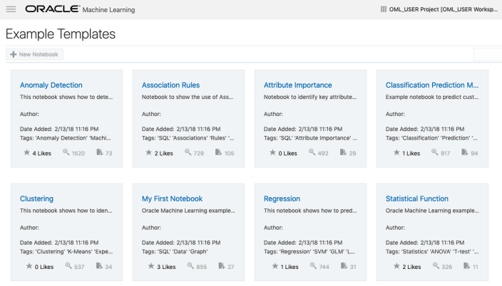
The above image shows the top part of the login screen for OML. To see the available sample notebooks click on the Examples icon. When you do, you will get the following sample OML Notebooks.
But what if you have a notebook you have used elsewhere. These can be exported in json format and loaded as a new notebook in OML.
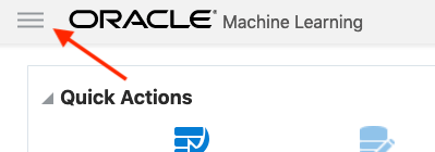
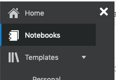
To load a new notebook into OML, select the icon (three horizontal line) on the top left hand corner of the screen. Then select Notebooks from the menu.
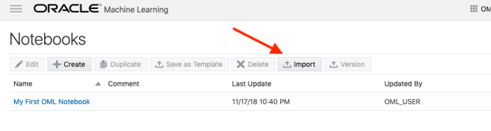
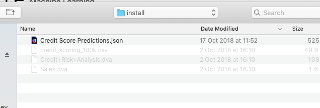
Then select the Import button located at the top of the Notebooks screen. This will open a File window, where you can select the json file from your file system.
A couple of seconds later the notebook will be available and listed along side any other notebooks you may have created.
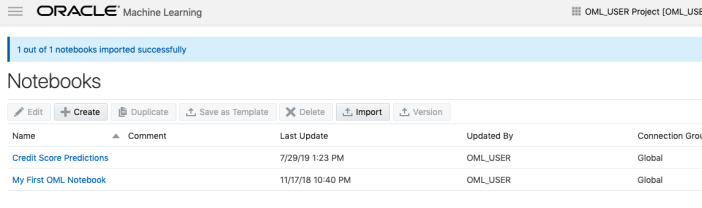
All done!
You have now imported a new notebook into OML and can now use it to process your data and perform machine learning using the in-database features.
Machine Learning on Mobile Devices
You: What? You can’t be serious? Machine Learning on Mobile Devices?
Me: The simple answer is ‘Yes you can!”
You: But, what about all the complex data processing, CPU or GPU, and everything else that is needed for machine learning?
Me: Yes you are correct, those things might not be needed. What’s the answer to everything in IT?
You: It Depends ?
Me: Exactly. Yes It Depends on what you are doing. In most cases you don’t need large amounts of machine processing power to do machine learning. Except if you are doing image processing. Then you do need a bit of power to support that work.
You: But how can a mobile device be used for machine learning?

Me: It Depends! 🙂 It depends on what you are doing. Most of the data processing power needed is for creating the models. That is what most people talk about. Very few people talk about the deployment of machine learning. Deployment, as in, using the machine learning models in your applications.
You: But why mobile devices? That sounds a bit silly?
Me: It does a bit. But when you think about it, how much do you use your mobile phone and tablet? Where else have you seen mobile devices being used?
You: I use these all the time, to do nearly everything. Just like everyone else I know.
Me: Exactly! and where else have you seen mobile devices being used?
You: Everywhere! hotels, bars, shops, hospitals, everywhere!
Me: Exactly. And it kind of makes sense to have machine learning scoring done at the point of capture of the data and not some hours or days or weeks later in some data warehouse or something else.
You: But what about the processing power of these devices. They aren’t powerful enough to run the machine learning models? Or are they?
Me: What is a machine learning model? In a simple way it is a mathematical formula of the data that calculates a particular outcome. Something that is a bit more complicated than using a sum function. Could a mobile device do that easily?
You: Yes. That should be really easy and fast for mobile devices? But machine learning is complex. People keep telling me how complex it is and how difficult it is!
Me: True it can be, but for most problems it can be as simple as writing a few lines of code to create a model. 3-4 lines of code in some languages. But the applying of the the machine learning model can be a simple task (maybe 1 line of code), although some simple data formatting might be needed, but that is a simple task too.
You: So, how can a machine learning model be run on a mobile device?
Me: Programmers write code to run applications on mobile devices. This code can be extended to include the machine learning model. This can be used to score or label the data or do some other processing. A few lines of code. A good alternative is to create a web service to all the remove scoring of the data.
You: The programming languages used for mobile development are a bit different to most other applications. Surely those mobile device languages don’t support machine learning.
Me: You’d be surprised by what’s available.
You: OK, What languages can I try? Where can I get started?
Me: Check out Firebase ML Kit, Apple CoreML and TensorFlow Lite. Those should be more than enough for you to get started with. There are a few others. But start with those.
You. Brilliant, thank you Brendan. I’ll let you know how I get on with those.
GoLang: Inserting records into Oracle Database using goracle
In this blog post I’ll give some examples of how to process data for inserting into a table in an Oracle Database. I’ve had some previous blog posts on how to setup and connecting to an Oracle Database, and another on retrieving data from an Oracle Database and the importance of setting the Array Fetch Size.
When manipulating data the statements can be grouped (generally) into creating new data and updating existing data.
When working with this kind of processing we need to avoid the creation of the statements as a concatenation of strings. This opens the possibility of SQL injection, plus we are not allowing the optimizer in the database to do it’s thing. Prepared statements allows for the reuse of execution plans and this in turn can speed up our data processing and applications.
In a previous blog post I gave a simple example of a prepared statement for querying data and then using it to pass in different values as a parameter to this statement.
dbQuery, err := db.Prepare("select cust_first_name, cust_last_name, cust_city from sh.customers where cust_gender = :1")
if err != nil {
    fmt.Println(err)
    return
}
defer dbQuery.Close()

rows, err := dbQuery.Query('M')
if err != nil {
    fmt.Println(".....Error processing query")
    fmt.Println(err)
    return
}
defer rows.Close()

var CustFname, CustSname,CustCity string
for rows.Next() {
    rows.Scan(&CustFname, &CustSname, &CustCity)
    fmt.Println(CustFname, CustSname, CustCity)
}
For prepared statements for inserting data we can follow a similar structure. In the following example a table call LAST_CONTACT is used. This table has columns:
- CUST_ID
- CON_METHOD
- CON_MESSAGE
_, err := db.Exec("insert into LAST_CONTACT(cust_id, con_method, con_message) VALUES(:1, :2, :3)", 1, "Phone", "First contact with customer")
if err != nil {
    fmt.Println(".....Error Inserting data")
    fmt.Println(err)
    return
}
an alternative is the following and allows us to get some additional information about what was done and the result from it. In this example we can get the number records processed.
stmt, err := db.Prepare("insert into LAST_CONTACT(cust_id, con_method, con_message) VALUES(:1, :2, :3)")
if err != nil {
    fmt.Println(err)
    return
}

res, err := dbQuery.Query(1, "Phone", "First contact with customer")
if err != nil {
    fmt.Println(".....Error Inserting data")
    fmt.Println(err)
    return
}

rowCnt := res.RowsAffected()
fmt.Println(rowCnt, " rows inserted.")
A similar approach can be taken for updating and deleting records
Managing Transactions
With transaction, a number of statements needs to be processed as a unit. For example, in double entry book keeping we have two inserts. One Credit insert and one debit insert. To do this we can define the start of a transaction using db.Begin() and the end of the transaction with a Commit(). Here is an example were we insert two contact details.
// start the transaction
transx, err := db.Begin()
if err != nil {
    fmt.Println(err)
    return
}

// Insert first record
_, err := db.Exec("insert into LAST_CONTACT(cust_id, con_method, con_message) VALUES(:1, :2, :3)", 1, "Email", "First Email with customer")
if err != nil {
    fmt.Println(".....Error Inserting data - first statement")
    fmt.Println(err)
    return
}
// Insert second record
_, err := db.Exec("insert into LAST_CONTACT(cust_id, con_method, con_message) VALUES(:1, :2, :3)", 1, "In-Person", "First In-Person with customer")
if err != nil {
    fmt.Println(".....Error Inserting data - second statement")
    fmt.Println(err)
    return
}

// complete the transaction
err = transx.Commit()
if err != nil {
    fmt.Println(".....Error Committing Transaction")
    fmt.Println(err)
    return
}
GoLang: Querying records from Oracle Database using goracle
Continuing my series of blog posts on using Go Lang with Oracle, in this blog I’ll look at how to setup a query, run the query and parse the query results. I’ll give some examples that include setting up the query as a prepared statement and how to run a query and retrieve the first record returned. Another version of this last example is a query that returns one row.
Check out my previous post on how to create a connection to an Oracle Database.
Let’s start with a simple example. This is the same example from the blog I’ve linked to above, with the Database connection code omitted.
    dbQuery := "select table_name from user_tables where table_name not like 'DM$%' and table_name not like 'ODMR$%'"
    rows, err := db.Query(dbQuery)
    if err != nil {
        fmt.Println(".....Error processing query")
        fmt.Println(err)
        return
    }
    defer rows.Close()

    fmt.Println("... Parsing query results")
    var tableName string
    for rows.Next() {
        rows.Scan(&tableName)
        fmt.Println(tableName)
    }
Processing a query and it’s results involves a number of steps and these are:
- Using Query() function to send the query to the database. You could check for errors when processing each row
- Iterate over the rows using Next()
- Read the columns for each row into variables using Scan(). These need to be defined because Go is strongly typed.
- Close the query results using Close(). You might want to defer the use of this function but depends if the query will be reused. The result set will auto close the query after it reaches the last records (in the loop). The Close() is there just in case there is an error and cleanup is needed.
You should never use * as a wildcard in your queries. Always explicitly list the attributes you want returned and only list the attributes you want/need. Never list all attributes unless you are going to use all of them. There can be major query performance benefits with doing this.
Now let us have a look at using prepared statement. With these we can parameterize the query giving us greater flexibility and reuse of the statements. Additionally, these give use better query execution and performance when run the the database as the execution plans can be reused.
    dbQuery, err := db.Prepare("select cust_first_name, cust_last_name, cust_city from sh.customers where cust_gender = :1")
    if err != nil {
        fmt.Println(err)
        return
    }
    defer dbQuery.Close()

    rows, err := dbQuery.Query('M')
    if err != nil {
        fmt.Println(".....Error processing query")
        fmt.Println(err)
        return
    }
    defer rows.Close()

    var CustFname, CustSname,CustCity string
    for rows.Next() {
        rows.Scan(&CustFname, &CustSname, &CustCity)
        fmt.Println(CustFname, CustSname, CustCity)
    }
Sometimes you may have queries that return only one row or you only want the first row returned by the query. In cases like this you can reduce the code to something like the following.
var CustFname, CustSname,CustCity string
err := db.Prepare("select cust_first_name, cust_last_name, cust_city from sh.customers where cust_gender = ?").Scan(&CustFname, &CustSname, &CustCity)
if err != nil {
    fmt.Println(err)
    return
}
fmt.Println(CustFname, CustSname, CustCity)
or an alternative to using Quer(), use QueryRow()
dbQuery, err := db.Prepare("select cust_first_name, cust_last_name, cust_city from sh.customers where cust_gender = ?")
if err != nil {
    fmt.Println(err)
    return
}
defer dbQuery.Close()

var CustFname, CustSname,CustCity string
err := dbQuery.QueryRow('M').Scan(&CustFname, &CustSname, &CustCity)
if err != nil {
    fmt.Println(".....Error processing query")
    fmt.Println(err)
    return
}
fmt.Println(CustFname, CustSname, CustCity)
Managing imbalanced Data Sets with SMOTE in Python
When working with data sets for machine learning, lots of these data sets and examples we see have approximately the same number of case records for each of the possible predicted values. In this kind of scenario we are trying to perform some kind of classification, where the machine learning model looks to build a model based on the input data set against a target variable. It is this target variable that contains the value to be predicted. In most cases this target variable (or feature) will contain binary values or equivalent in categorical form such as Yes and No, or A and B, etc or may contain a small number of other possible values (e.g. A, B, C, D).
For the classification algorithm to perform optimally and be able to predict the possible value for a new case record, it will need to see enough case records for each of the possible values. What this means, it would be good to have approximately the same number of records for each value (there are many ways to overcome this and these are outside the score of this post). But most data sets, and those that you will encounter in real life work scenarios, are never balanced, as in having a 50-50 split. What we typically encounter might be a 90-10, 98-2, etc type of split. These data sets are said to be imbalanced.

The image above gives examples of two approaches for creating a balanced data set. The first is under-sampling. This involves reducing the class that contains the majority of the case records and reducing it to match the number of case records in the minor class. The problems with this include, the resulting data set is too small to be meaningful, the case records removed could contain important records and scenarios that the model will need to know about.
The second example is creating a balanced data set by increasing the number of records in the minority class. There are a few approaches to creating this. The first approach is to create duplicate records, from the minor class, until such time as the number of case records are approximately the same for each class. This is the simplest approach. The second approach is to create synthetic records that are statistically equivalent of the original data set. A commonly technique used for this is called SMOTE, Synthetic Minority Oversampling Technique. SMOTE uses a nearest neighbors algorithm to generate new and synthetic data we can use for training our model. But one of the issues with SMOTE is that it will not create sample records outside the bounds of the original data set. As you can image this would be very difficult to do.
The following examples will illustrate how to perform Under-Sampling and Over-Sampling (duplication and using SMOTE) in Python using functions from Pandas, Imbalanced-Learn and Sci-Kit Learn libraries.
NOTE: The Imbalanced-Learn library (e.g. SMOTE)requires the data to be in numeric format, as it statistical calculations are performed on these. The python function get_dummies was used as a quick and simple to generate the numeric values. Although this is perhaps not the best method to use in a real project. With the other sampling functions can process data sets with a sting and numeric.
Data Set: Is the Portuaguese Banking data set and is available on the UCI Data Set Repository, and many other sites. Here are some basics with that data set.
import warnings

import pandas as pd
import numpy as np
import matplotlib.pyplot as plt
get_ipython().magic('matplotlib inline')

bank_file = ".../bank-additional-full.csv"

# import dataset
df = pd.read_csv(bank_file, sep=';',)

# get basic details of df (num records, num features)
df.shape
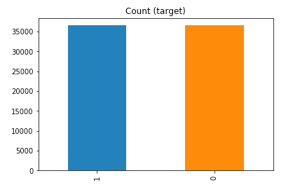
df['y'].value_counts() # dataset is imbalanced with majority of class label as "no".
no     36548
yes     4640
Name: y, dtype: int64
#print bar chart
df.y.value_counts().plot(kind='bar', title='Count (target)');

Example 1a – Down/Under sampling the majority class y=1 (using random sampling)
count_class_0, count_class_1 = df.y.value_counts()

# Divide by class
df_class_0 = df[df['y'] == 0] #majority class
df_class_1 = df[df['y'] == 1] #minority class

# Sample Majority class (y=0, to have same number of records as minority calls (y=1)
df_class_0_under = df_class_0.sample(count_class_1)
# join the dataframes containing y=1 and y=0
df_test_under = pd.concat([df_class_0_under, df_class_1])

print('Random under-sampling:')
print(df_test_under.y.value_counts())
print("Num records = ", df_test_under.shape[0])

df_test_under.y.value_counts().plot(kind='bar', title='Count (target)');
Example 1b – Down/Under sampling the majority class y=1 using imblearn
from imblearn.under_sampling import RandomUnderSampler

X = df_new.drop('y', axis=1)
Y = df_new['y']

rus = RandomUnderSampler(random_state=42, replacement=True)
X_rus, Y_rus = rus.fit_resample(X, Y)

df_rus = pd.concat([pd.DataFrame(X_rus), pd.DataFrame(Y_rus, columns=['y'])], axis=1)

print('imblearn over-sampling:')
print(df_rus.y.value_counts())
print("Num records = ", df_rus.shape[0])

df_rus.y.value_counts().plot(kind='bar', title='Count (target)');
[same results as Example 1a]
Example 1c – Down/Under sampling the majority class y=1 using Sci-Kit Learn
from sklearn.utils import resample

print("Original Data distribution")
print(df['y'].value_counts())

# Down Sample Majority class
down_sample = resample(df[df['y']==0],
replace = True, # sample with replacement
n_samples = df[df['y']==1].shape[0], # to match minority class
random_state=42) # reproducible results

# Combine majority class with upsampled minority class
train_downsample = pd.concat([df[df['y']==1], down_sample])

# Display new class counts
print('Sci-Kit Learn : resample : Down Sampled data set')
print(train_downsample['y'].value_counts())
print("Num records = ", train_downsample.shape[0])
train_downsample.y.value_counts().plot(kind='bar', title='Count (target)');
[same results as Example 1a]
Example 2 a – Over sampling the minority call y=0 (using random sampling)
df_class_1_over = df_class_1.sample(count_class_0, replace=True)
df_test_over = pd.concat([df_class_0, df_class_1_over], axis=0)
print('Random over-sampling:')
print(df_test_over.y.value_counts())
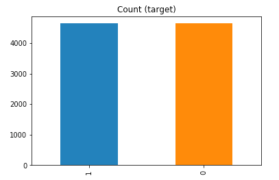
df_test_over.y.value_counts().plot(kind='bar', title='Count (target)');
Random over-sampling:
1    36548
0    36548
Name: y, dtype: int64
Example 2b – Over sampling the minority call y=0 using SMOTE
from imblearn.over_sampling import SMOTE

print(df_new.y.value_counts())
X = df_new.drop('y', axis=1)
Y = df_new['y']

sm = SMOTE(random_state=42)
X_res, Y_res = sm.fit_resample(X, Y)

df_smote_over = pd.concat([pd.DataFrame(X_res), pd.DataFrame(Y_res, columns=['y'])], axis=1)

print('SMOTE over-sampling:')
print(df_smote_over.y.value_counts())

df_smote_over.y.value_counts().plot(kind='bar', title='Count (target)');
[same results as Example 2a]
Example 2c – Over sampling the minority call y=0 using Sci-Kit Learn
from sklearn.utils import resample

print("Original Data distribution")
print(df['y'].value_counts())

# Upsample minority class
train_positive_upsample = resample(df[df['y']==1],
replace = True, # sample with replacement
n_samples = train_zero.shape[0], # to match majority class
random_state=42) # reproducible results

# Combine majority class with upsampled minority class
train_upsample = pd.concat([train_negative, train_positive_upsample])

# Display new class counts
print('Sci-Kit Learn : resample : Up Sampled data set')
print(train_upsample['y'].value_counts())
train_upsample.y.value_counts().plot(kind='bar', title='Count (target)');
[same results as Example 2a]
Embedding Transformation Data Pipeline into ML Model using Oracle Data Mining
I’ve written several blog posts about how to use the DBMS_DATA_MINING.TRANSFORM function to create various data transformations and how to apply these to your data. All of these steps can be simple enough to following and re-run in a lab environment. But the real value with data science and machine learning comes when you deploy the models into production and have the ML models scoring data as it is being produced, and your applications acting upon these predictions immediately, and not some hours or days later when the data finally arrives in the lab environment.
It would be useful to be able to bundle all the transformations into the same process the create the model. The transformations and model become one, together. If this is possible, then that greatly simplifies how the ML model can be deployed into production. It then becomes a simple function or REST call. We need to keep this simple (KISS).
Using the examples from my previous blog posts performing various data transformations, the following example shows how you can bundle these up into one defined set of transformations and then embed these transformations as part of the ML model. To do this we need to define a list of transformations. We can do this using:
xform_list IN TRANSFORM_LIST DEFAULT NULL
Where TRANSFORM_LIST has the following structure:
TRANFORM_REC IS RECORD (
     attribute_name       VARCHAR2(4000),
     attribute_subname    VARCHAR2(4000),
     expression           EXPRESSION_REC,
     reverse_expression   EXPRESSION_REC,
     attribute_spec       VARCHAR2(4000));
You can use the DBMS_DATA_MINING.SET_TRANSFORM function to defined the transformations. The following example illustrates the transformation of converting the BOOKKEEPING_APPLICATION attribute from a number data type to a character data type.
DECLARE
   transform_stack   dbms_data_mining_transform.TRANSFORM_LIST;
BEGIN
   dbms_data_mining_transform.SET_TRANSFORM(transform_stack,
                                  'BOOKKEEPING_APPLICATION',
                                  NULL,
                                  'to_char(BOOKKEEPING_APPLICATION)',
                                  'to_number(BOOKKEEPING_APPLICATION)',
                                  NULL);
END;
Alternatively you can use the SET_EXPRESSION function and then create the transformation using it.
You can Stack the transforms together. Using the above example you could express a number of transformations and have these stored in the TRANSFORM_STACK variable. You can then pass this variable into your CREATE_MODEL procedure and have these transformations embedded in your ML model.
DECLARE
   transform_stack   dbms_data_mining_transform.TRANSFORM_LIST;
BEGIN
   -- Define the transformation list
   dbms_data_mining_transform.SET_TRANSFORM(transform_stack,
                                  'BOOKKEEPING_APPLICATION',
                                  NULL,
                                  'to_char(BOOKKEEPING_APPLICATION)',
                                  'to_number(BOOKKEEPING_APPLICATION)',
                                  NULL);

   -- Create the data mining model
   DBMS_DATA_MINING.CREATE_MODEL(
      model_name           => 'DEMO_TRANSFORM_MODEL',
      mining_function      => dbms_data_mining.classification,
      data_table_name      => 'MINING_DATA_BUILD_V',
      case_id_column_name  => 'cust_id',
      target_column_name   => 'affinity_card',
      settings_table_name  => 'demo_class_dt_settings',
      xform_list           => transform_stack);
END;
My previous blog posts showed how to create various types of transformations. These transformations were then used to create a view of the data set that included these transformations. To embed these transformations in the ML Model we need to use the STACK function. The following examples illustrate the stacking of the transformations created in the previous blog posts. These transformations are added (or stacked) to a transformation list and then added to the CREATE_MODEL function, embedding these transformations in the model.
DECLARE
   transform_stack   dbms_data_mining_transform.TRANSFORM_LIST;
BEGIN
   -- Stack the missing numeric transformations
   dbms_data_mining_transform.STACK_MISS_NUM (
          miss_table_name   => 'TRANSFORM_MISSING_NUMERIC',
          xform_list        => transform_stack);

   -- Stack the missing categorical transformations
   dbms_data_mining_transform.STACK_MISS_CAT (
          miss_table_name   => 'TRANSFORM_MISSING_CATEGORICAL',
          xform_list        => transform_stack);

   -- Stack the outlier treatment for AGE
   dbms_data_mining_transform.STACK_CLIP (
          clip_table_name   => 'TRANSFORM_OUTLIER',
          xform_list        => transform_stack);

   -- Stack the normalization transformation
   dbms_data_mining_transform.STACK_NORM_LIN (
          norm_table_name   => 'MINING_DATA_NORMALIZE',
          xform_list        => transform_stack);

   -- Create the data mining model
   DBMS_DATA_MINING.CREATE_MODEL(
      model_name           => 'DEMO_STACKED_MODEL',
      mining_function      => dbms_data_mining.classification,
      data_table_name      => 'MINING_DATA_BUILD_V',
      case_id_column_name => 'cust_id',
      target_column_name   => 'affinity_card',
      settings_table_name => 'demo_class_dt_settings',
      xform_list           => transform_stack);
END;
To view the embedded transformations in your data mining model you can use the GET_MODEL_TRANSFORMATIONS function.
SELECT TO_CHAR(expression)
FROM TABLE (dbms_data_mining.GET_MODEL_TRANSFORMATIONS('DEMO_STACKED_MODEL'));
TO_CHAR(EXPRESSION)
--------------------------------------------------------------------------------
(CASE  WHEN (NVL("AGE",38.892)<18) THEN 18 WHEN (NVL("AGE",38.892)>70) THEN 70 E
LSE NVL("AGE",38.892) END -18)/52

NVL("BOOKKEEPING_APPLICATION",.880667)
NVL("BULK_PACK_DISKETTES",.628)
NVL("FLAT_PANEL_MONITOR",.582)
NVL("HOME_THEATER_PACKAGE",.575333)
NVL("OS_DOC_SET_KANJI",.002)
NVL("PRINTER_SUPPLIES",1)
(CASE  WHEN (NVL("YRS_RESIDENCE",4.08867)<1) THEN 1 WHEN (NVL("YRS_RESIDENCE",4.
08867)>8) THEN 8 ELSE NVL("YRS_RESIDENCE",4.08867) END -1)/7

NVL("Y_BOX_GAMES",.286667)
NVL("COUNTRY_NAME",'United States of America')
NVL("CUST_GENDER",'M')
NVL("CUST_INCOME_LEVEL",'J: 190,000 - 249,999')
NVL("CUST_MARITAL_STATUS",'Married')
NVL("EDUCATION",'HS-grad')
NVL("HOUSEHOLD_SIZE",'3')
NVL("OCCUPATION",'Exec.')
Importance of setting Fetched Rows size for Database Query using Golang
When issuing queries to the database one of the challenges every developer faces is how to get the results quickly. If your queries are only returning a small number of records, eg. < 5, then you don’t really have to worry about execution time. That is unless your query is performing some complex processing, joining lots of tables, etc.
Most of the time developers are working with one or a small number of records, using a simple query. Everything runs quickly.
But what if your query is returning several tens or thousands of records. Assuming we have a simple query and no query optimization is needed, the challenge facing the developer is how can you get all of those records quickly into your environment and process them. Typically the database gets blamed for the query result set being returned slowly. But what if this wasn’t the case? In most cases developers take the default parameter settings of the functions and libraries. For database connection libraries and their functions, you can change some of the parameters and affect how your code, your query, gets executed on the Database server and can affect how quickly the data is shipped from the database to your code.
One very important parameter to consider is the query array size. This is the number of records the database will send to your code in each batch. The database will keep sending batches until you tell it to stop. It makes sense to have the size of this batch set to a small value, as most queries return one or a small number of records. But when we get onto returning a larger number of records it can affect the response time significantly.
I tested the effect of changing the size of the returning buffer/array using Golang and querying data in an Oracle Database, hosted on Oracle Cloud, and using goracle library to connect to the database.
[ I did a similar test using Python. The results can be found here. You will notices that Golang is significantly quicker than Python, as you would expect. ]
The database table being queried contains 55,000 records and I just executed a SELECT * FROM … on this table. The results shown below contain the timing the query took to process this data for different buffer/array sizes by setting the FetchRowCount value.
rows, err := db.Query(dbQuery, goracle.FetchRowCount(arraySize))

As you can see, as the size of the buffer/array size increases the timing it takes to process the data drops. This is because the buffer/array is returning a larger number of records, and this results in a reduced number of round trips to/from the database i.e. fewer packets of records are sent across the network.
The challenge for the developer is to work out the optimal number to set for the buffer/array size. The default for the goracle libary, using Oracle client is 256 row/records.
When that above query is run, without the FetchRowCount setting, it will use this default 256 value. When this is used we get the following timings.

We can see, for the data set being used in this test case the optimal setting needs to be around 1,500.
What if we set the parameter to be very large? That would no necessarily make it quicker. You can see from the first table the timing starts to increase for the last two settings. There is an overhead in gathering and sending the data.
Here is a subset of the Golang code I used to perform the tests.
var currentTime = time.Now()

var i int

var custId int

arrayOne := [11] int{5, 10, 30, 50, 100, 200, 500, 1000, 1500, 2000, 2500}


currentTime = time.Now()


fmt.Println("Array Size = ", arraySize, " : ", currentTime.Format("03:04:05:06 PM"))


for index, arraySize := range arrayOne {

    currentTime = time.Now()

    fmt.Println(index, " Array Size = ", arraySize, " : ", currentTime.Format("03:04:05:06 PM"))


    db, err := sql.Open("goracle", username+"/"+password+"@"+host+"/"+database)

    if err != nil {

        fmt.Println("... DB Setup Failed")

        fmt.Println(err)

        return

    }

    defer db.Close()


    if err = db.Ping(); err != nil {

        fmt.Printf("Error connecting to the database: %s\n", err)

        return

    }


    currentTime = time.Now()

    fmt.Println("...Executing Query", currentTime.Format("03:04:05:06 PM"))

    dbQuery := "select cust_id from sh.customers"

    rows, err := db.Query(dbQuery, goracle.FetchRowCount(arraySize))

    if err != nil {

        fmt.Println(".....Error processing query")

        fmt.Println(err)

        return

    }

    defer rows.Close()


    i = 0

    currentTime = time.Now()

    fmt.Println("... Parsing query results", currentTime.Format("03:04:05:06 PM"))

   for rows.Next() {

        rows.Scan(&custId)

        i++

        if i% 10000 == 0 {

            currentTime = time.Now()

            fmt.Println("...... ",i, " customers processed", currentTime.Format("03:04:05:06 PM"))

        }

    }


    currentTime = time.Now()

    fmt.Println(i, " customers processed", currentTime.Format("03:04:05:06 PM"))


    fmt.Println("... Closing connection")

    finishTime := time.Now()

    fmt.Println("Finished at ", finishTime.Format("03:04:05:06 PM"))


}
Transforming Outliers in Oracle Data Mining
In previous posts I’ve shown how to use the DBMS_DATA_MINING.TRANSFORM function to transform data is various ways including, normalization and missing data. In this post I’ll build upon these to show how to outliers can be handled.
The following example will show you how you can transform data to identify outliers and transform them. In the example, Winsorsizing transformation is performed where the outlier values are replaced by the nearest value that is not an outlier.
The transformation process takes place in three stages. For the first stage a table is created to contain the outlier transformation data. The second stage calculates the outlier transformation data and store these in the table created in stage 1. One of the parameters to the outlier procedure requires you to list the attributes you do not the transformation procedure applied to (this is instead of listing the attributes you do want it applied to). The third stage is to create a view (MINING_DATA_V_2) that contains the data set with the outlier transformation rules applied. The input data set to this stage can be the output from a previous transformation process (e.g. DATA_MINING_V).
BEGIN
   -- Clean-up : Drop the previously created tables
   BEGIN
      execute immediate 'drop table TRANSFORM_OUTLIER';
   EXCEPTION
      WHEN others THEN
         null;
   END;

   -- Stage 1 : Create the table for the transformations
   -- Perform outlier treatment for: AGE and YRS_RESIDENCE
   --
   DBMS_DATA_MINING_TRANSFORM.CREATE_CLIP (
      clip_table_name => 'TRANSFORM_OUTLIER');

   -- Stage 2 : Transform the categorical attributes
   --   Exclude the number attributes you do not want transformed
   DBMS_DATA_MINING_TRANSFORM.INSERT_CLIP_WINSOR_TAIL (
      clip_table_name => 'TRANSFORM_OUTLIER',
      data_table_name => 'MINING_DATA_V',
      tail_frac       => 0.025,
      exclude_list    => DBMS_DATA_MINING_TRANSFORM.COLUMN_LIST (
                          'affinity_card',
                          'bookkeeping_application',
                          'bulk_pack_diskettes',
                          'cust_id',
                          'flat_panel_monitor',
                          'home_theater_package',
                          'os_doc_set_kanji',
                          'printer_supplies',
                          'y_box_games'));

   -- Stage 3 : Create the view with the transformed data
   DBMS_DATA_MINING_TRANSFORM.XFORM_CLIP(
      clip_table_name => 'TRANSFORM_OUTLIER',
      data_table_name => 'MINING_DATA_V',
      xform_view_name => 'MINING_DATA_V_2');
END;
The view MINING_DATA_V_2 will now contain the data from the original data set transformed to process missing data for numeric and categorical data (from previous blog post), and also has outlier treatment for the AGE attribute.

You must be logged in to post a comment.