
OCI Data Labeling using Bounding Box
In a previous post, I gave examples of how to label data using OCI Data Labeling. It was a simple approach to data labeling images for input to AI Vision. In that post, we just gave a label for the image to indicate if the image contained a Cat or a Dog. Yes, that’s a very simple approach, and we can build image classification models, and use the resulting model to predict a label for new images. These would be labeled as a Cat or a Dog with a degree of certainty. Although this simple approach can give OK-ish results, we typically want a more detailed model and predictions. For a more detailed approach, we can use Object Detection. For this, we need to prepare our data set in a slightly different way and Yes it does take a bit more time to prepare. Or perhaps it takes a lot more time to prepare the data. But this extra time in preparing the data should (in theory) give us a more accurate model.
This post will focus on creating a new labeled dataset using bounding boxes, and in a later post, we’ll examine the resulting model to see if it gives better or more accurate results.
I’ve mentioned the phrase ‘bounding box’ a few times and this approach does exactly as the phrase indicates. Draw a box around the object and assign a label to it. In our example, we have used a Cats and Dogs dataset. We’ll use that same dataset (50 images of each animal). This approach to labelling the images takes much longer to complete, as we have to draw a box around each animal. But it is worth the effort, as the models can focus on what is inside the box and ignore anything outside the box.
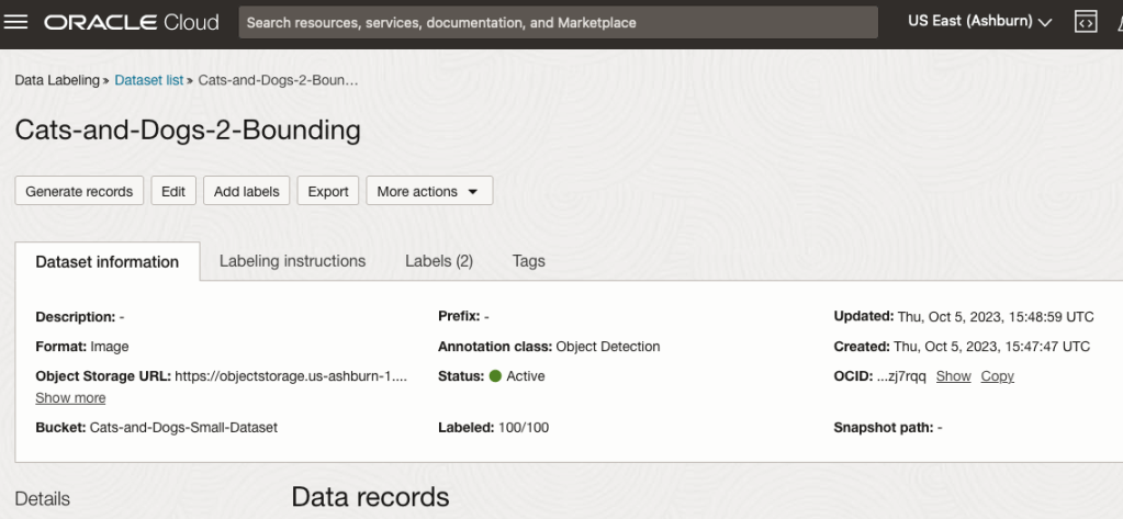
The first task is to define the dataset that will contain our newly labelled data based on the bound box method.
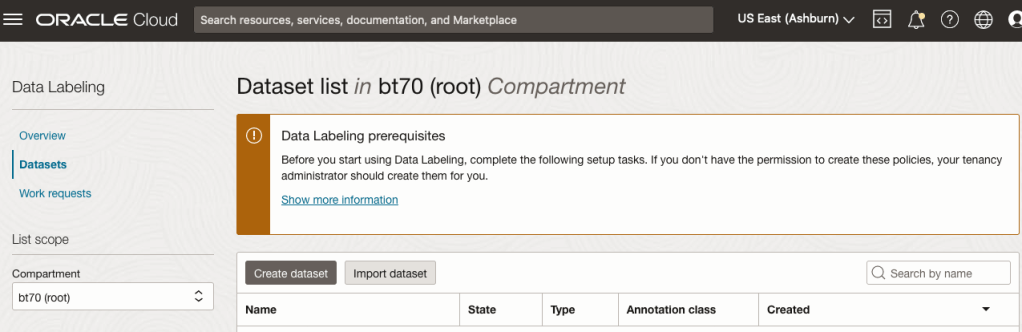
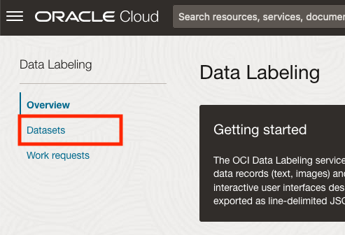
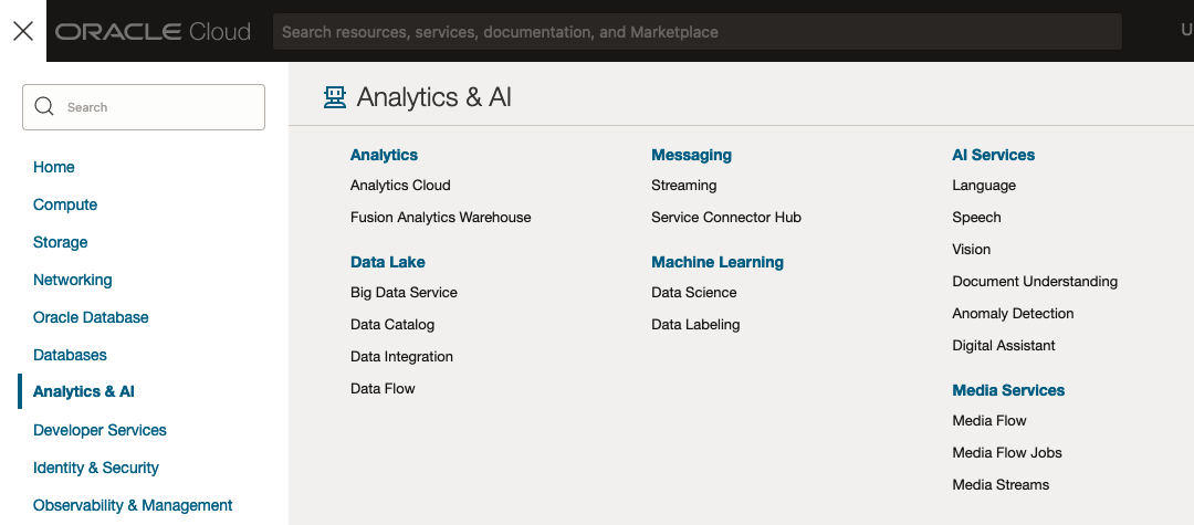
From the OCI menu, go to the Analytics & AI section and select Data Labeling.
Select the Dataset menu items(on the left hand side of the screen, and then click on the Create dataset button.
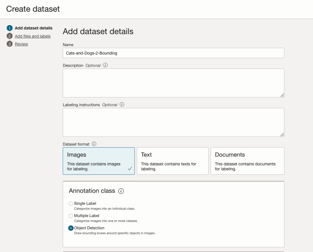
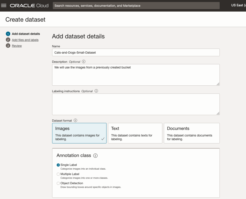
The Add Dataset screen allows us to enter the details of the dataset we want to use.
Our dataset is based on a dataset in Object storage, and we can define it as the basis of creating a newly labelled dataset. This does not affect the underlying original dataset.
In this case, we want to select Object Detection in the section called Annotation Class.
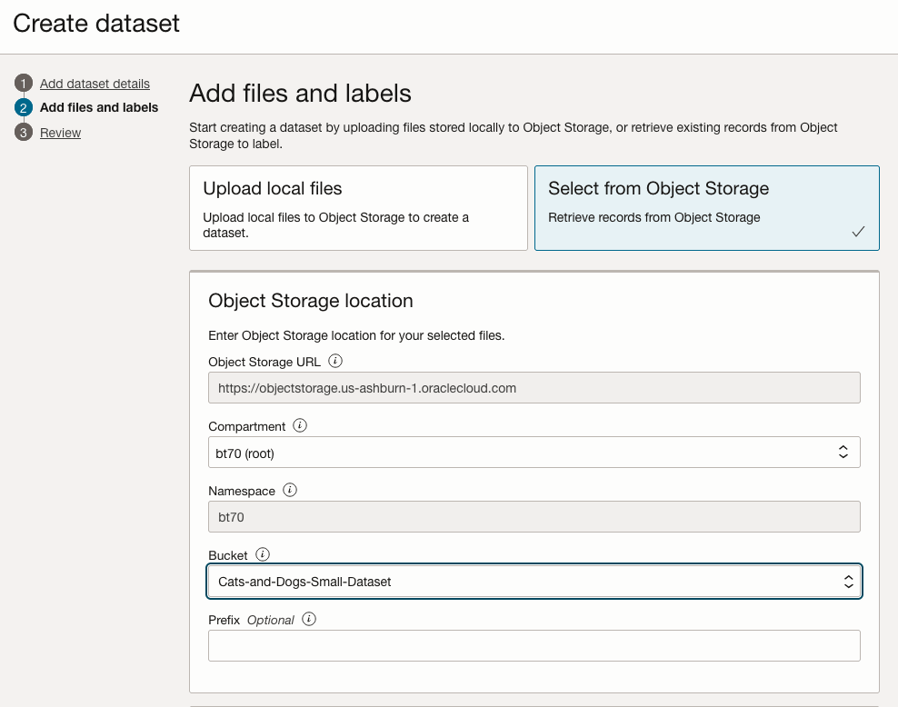
On the next screen, you can define the Bucket containing the images we want to label.
In our case, we will be using the Cats and Dogs dataset previously loaded into Object Storage.
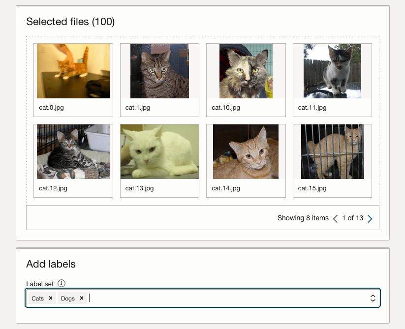
In the next section, it will tell you how many files are part of the underlying dataset. By default, it will use all of them.
Add the labels you want to use, although you can add more during the labelling process.
Click Next to move to the next screen and then Click Finish to complete this setup.
After a moments, depending on the number of images in the underlying dataset, the version of the dataset for labelling can now be processed.
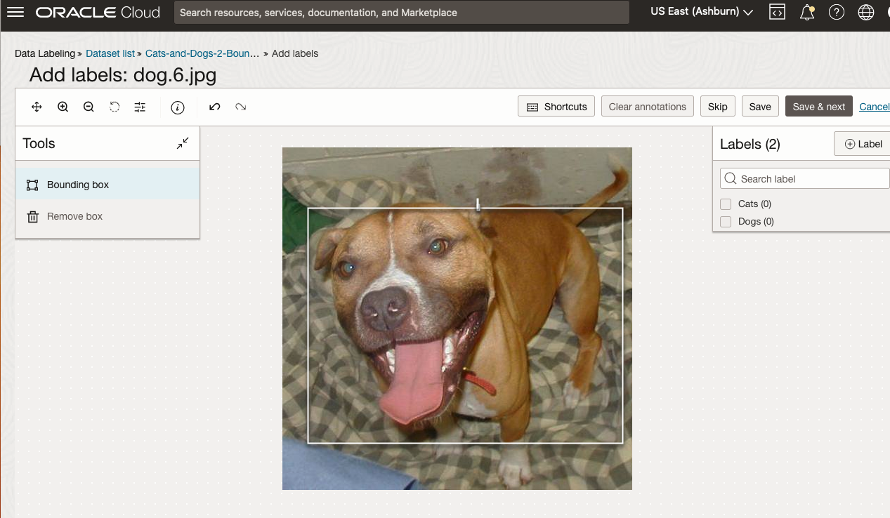
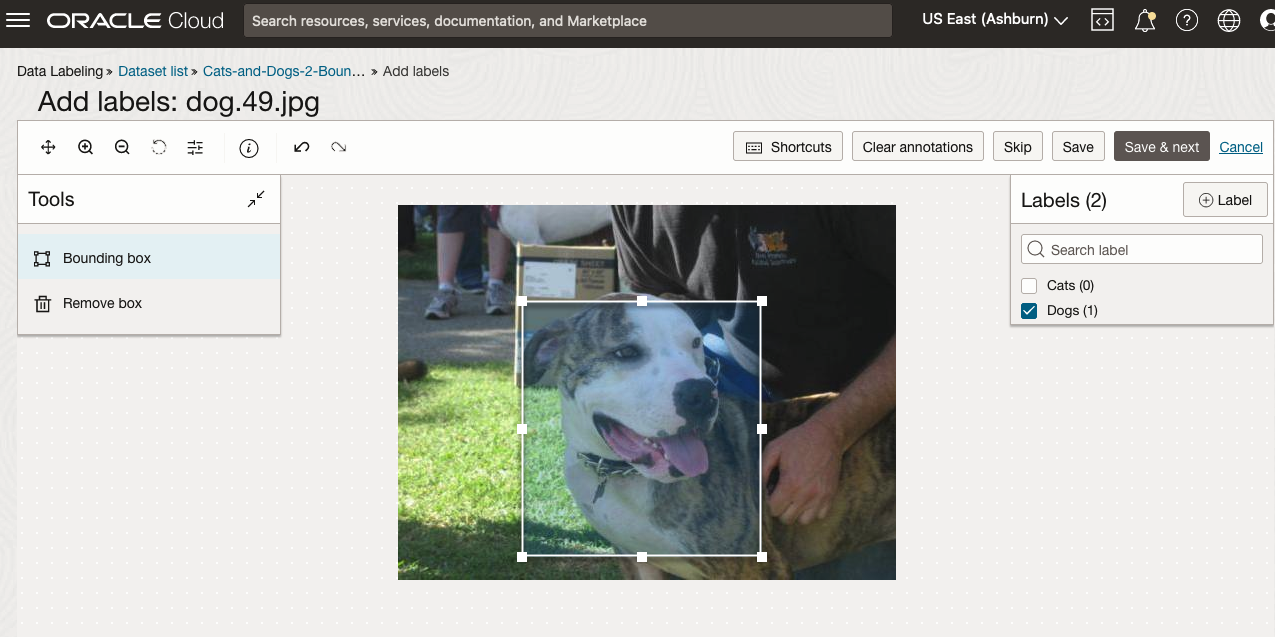
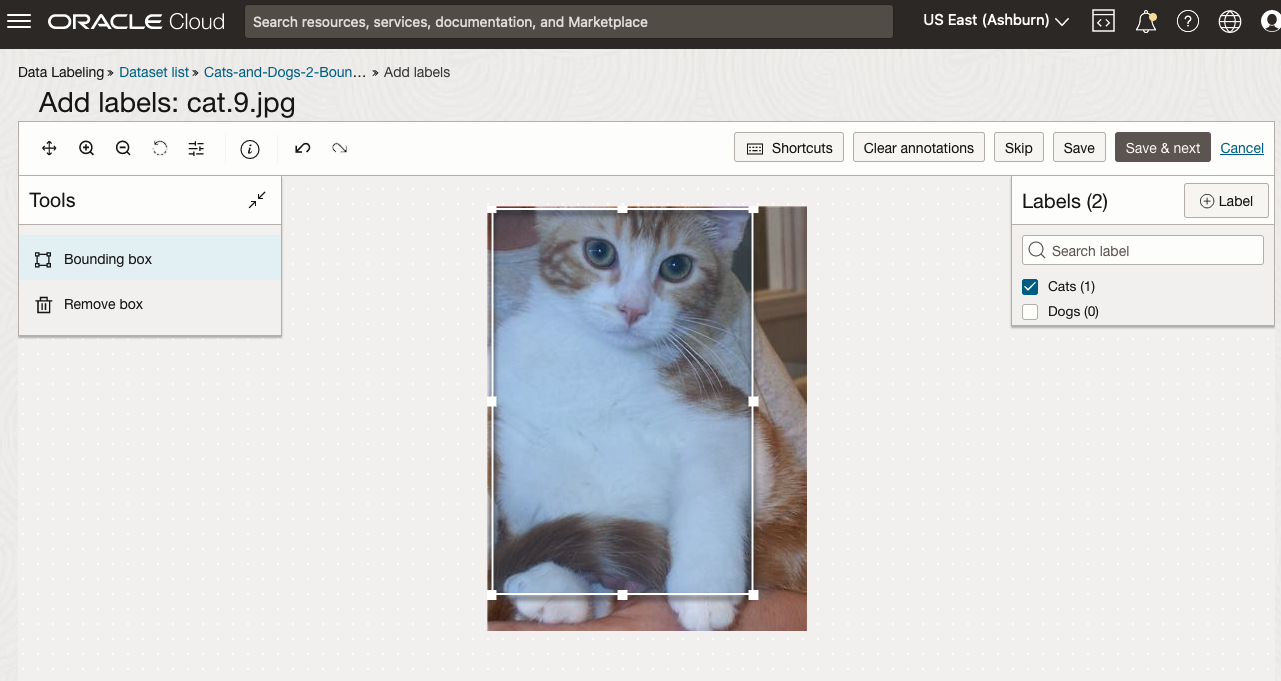
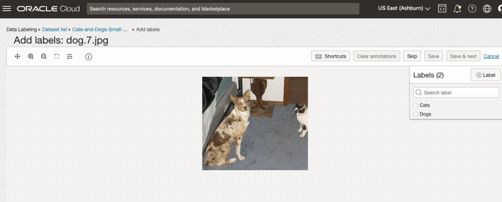
To stat the labelling process, click on the first on the first image. Using your mouse drag a box over the main item you want to label. In my example, I’m drawing a box around the animals while trying to exclude as much of the surrounding and background parts of the image. After drawing the box, you can then select the label, from the list on the right-hand side of the screen and then click the Save & Next button. Continue doing this until you complete all images. Yes this can take some time, but it should help OCI Vision create a better-informed model for these animals

Dictionary Health Check in 23ai Oracle Database
There’s a new PL/SQL package in Oracle 23ai Database that allows you to check for any inconsistencies or problems that might occur in the data dictionary of the database. Previously there was an external SQL script available to perform similar action (hcheck.sql).
Inconsistencies can occur from time to time and can be caused by various reasons. It’s good to perform regular checks, and having the necessary functionality in a PL/SQL package allows for easier use and automation.
Warning: There are slightly different names for this PL/SQL package and it depends on which version of 23ai Database you are running. If you are running an early release of 23c this package is called DBMS_HCHECK. If you are running against a newer version (say 23.3ai) the package is called DBMS_DICTIONARY_CHECK.
This PL/SQL package assists you in identifying such inconsistencies and in some cases provides guided remediation to resolve the problem and avoid such database failures.
The following illustrates how to use the main functions in the package and these are being run on a 23ai (Free) Database running in Docker. The main functions include FULL and CRITICAL. There are an additional 66 functions which allow you to examine each of the report elements returned in the FULL report.
To run the FULL report
exec dbms_dictionary_check.full

dbms_hcheck on 02-OCT-2023 13:56:39
----------------------------------------------
Catalog Version 23.0.0.0.0 (2300000000)
db_name: FREE
Is CDB?: YES CON_ID: 3 Container: FREEPDB1
Trace File: /opt/oracle/diag/rdbms/free/FREE/trace/FREE_ora_335_HCHECK.trc

                                   Catalog       Fixed
Procedure Name                     Version    Vs Release    Timestamp      Result
------------------------------ ... ---------- -- ---------- -------------- ------
.- OIDOnObjCol                 ... 2300000000 <=  *All Rel* 10/02 13:56:39 PASS
.- LobNotInObj                 ... 2300000000 <=  *All Rel* 10/02 13:56:40 PASS
.- SourceNotInObj              ... 2300000000 <=  *All Rel* 10/02 13:56:40 PASS
.- OversizedFiles              ... 2300000000 <=  *All Rel* 10/02 13:56:40 PASS
.- PoorDefaultStorage          ... 2300000000 <=  *All Rel* 10/02 13:56:40 PASS
.- PoorStorage                 ... 2300000000 <=  *All Rel* 10/02 13:56:40 PASS
.- TabPartCountMismatch        ... 2300000000 <=  *All Rel* 10/02 13:56:41 PASS
.- TabComPartObj               ... 2300000000 <=  *All Rel* 10/02 13:56:41 PASS
.- Mview                       ... 2300000000 <=  *All Rel* 10/02 13:56:41 PASS
.- ValidDir                    ... 2300000000 <=  *All Rel* 10/02 13:56:41 PASS
.- DuplicateDataobj            ... 2300000000 <=  *All Rel* 10/02 13:56:41 PASS
.- ObjSyn                      ... 2300000000 <=  *All Rel* 10/02 13:56:43 PASS
.- ObjSeq                      ... 2300000000 <=  *All Rel* 10/02 13:56:43 PASS
.- UndoSeg                     ... 2300000000 <=  *All Rel* 10/02 13:56:43 PASS
.- IndexSeg                    ... 2300000000 <=  *All Rel* 10/02 13:56:43 PASS
.- IndexPartitionSeg           ... 2300000000 <=  *All Rel* 10/02 13:56:44 PASS
.- IndexSubPartitionSeg        ... 2300000000 <=  *All Rel* 10/02 13:56:44 PASS
.- TableSeg                    ... 2300000000 <=  *All Rel* 10/02 13:56:44 PASS
.- TablePartitionSeg           ... 2300000000 <=  *All Rel* 10/02 13:56:44 PASS
.- TableSubPartitionSeg        ... 2300000000 <=  *All Rel* 10/02 13:56:44 PASS
.- PartCol                     ... 2300000000 <=  *All Rel* 10/02 13:56:44 PASS
.- ValidSeg                    ... 2300000000 <=  *All Rel* 10/02 13:56:44 PASS
.- IndPartObj                  ... 2300000000 <=  *All Rel* 10/02 13:56:44 PASS
.- DuplicateBlockUse           ... 2300000000 <=  *All Rel* 10/02 13:56:44 PASS
.- FetUet                      ... 2300000000 <=  *All Rel* 10/02 13:56:44 PASS
.- Uet0Check                   ... 2300000000 <=  *All Rel* 10/02 13:56:44 PASS
.- SeglessUET                  ... 2300000000 <=  *All Rel* 10/02 13:56:44 PASS
.- ValidInd                    ... 2300000000 <=  *All Rel* 10/02 13:56:44 PASS
.- ValidTab                    ... 2300000000 <=  *All Rel* 10/02 13:56:44 PASS
.- IcolDepCnt                  ... 2300000000 <=  *All Rel* 10/02 13:56:44 PASS
.- ObjIndDobj                  ... 2300000000 <=  *All Rel* 10/02 13:56:45 PASS
.- TrgAfterUpgrade             ... 2300000000 <=  *All Rel* 10/02 13:56:45 PASS
.- ObjType0                    ... 2300000000 <=  *All Rel* 10/02 13:56:45 PASS
.- ValidOwner                  ... 2300000000 <=  *All Rel* 10/02 13:56:45 PASS
.- StmtAuditOnCommit           ... 2300000000 <=  *All Rel* 10/02 13:56:45 PASS
.- PublicObjects               ... 2300000000 <=  *All Rel* 10/02 13:56:46 PASS
.- SegFreelist                 ... 2300000000 <=  *All Rel* 10/02 13:56:46 PASS
.- ValidDepends                ... 2300000000 <=  *All Rel* 10/02 13:56:46 PASS
.- CheckDual                   ... 2300000000 <=  *All Rel* 10/02 13:56:47 PASS
.- ObjectNames                 ... 2300000000 <=  *All Rel* 10/02 13:56:47 PASS
.- ChkIotTs                    ... 2300000000 <=  *All Rel* 10/02 13:56:51 PASS
.- NoSegmentIndex              ... 2300000000 <=  *All Rel* 10/02 13:56:51 PASS
.- NextObject                  ... 2300000000 <=  *All Rel* 10/02 13:56:51 PASS
.- DroppedROTS                 ... 2300000000 <=  *All Rel* 10/02 13:56:51 PASS
.- FilBlkZero                  ... 2300000000 <=  *All Rel* 10/02 13:56:51 PASS
.- DbmsSchemaCopy              ... 2300000000 <=  *All Rel* 10/02 13:56:51 PASS
.- IdnseqObj                   ... 2300000000 >  1201000000 10/02 13:56:51 PASS
.- IdnseqSeq                   ... 2300000000 >  1201000000 10/02 13:56:51 PASS
.- ObjError                    ... 2300000000 >  1102000000 10/02 13:56:51 PASS
.- ObjNotLob                   ... 2300000000 <=  *All Rel* 10/02 13:56:51 PASS
.- MaxControlfSeq              ... 2300000000 <=  *All Rel* 10/02 13:56:51 PASS
.- SegNotInDeferredStg         ... 2300000000 >  1102000000 10/02 13:56:52 PASS
.- SystemNotRfile1             ... 2300000000 <=  *All Rel* 10/02 13:56:52 PASS
.- DictOwnNonDefaultSYSTEM     ... 2300000000 <=  *All Rel* 10/02 13:56:53 PASS
.- ValidateTrigger             ... 2300000000 <=  *All Rel* 10/02 13:56:53 PASS
.- ObjNotTrigger               ... 2300000000 <=  *All Rel* 10/02 13:56:54 PASS
.- InvalidTSMaxSCN             ... 2300000000 >  1202000000 10/02 13:56:54 PASS
.- OBJRecycleBin               ... 2300000000 <=  *All Rel* 10/02 13:56:54 PASS
---------------------------------------
02-OCT-2023 13:56:54  Elapsed: 15 secs
---------------------------------------
Found 0 potential problem(s) and 0 warning(s)

Trace File: /opt/oracle/diag/rdbms/free/FREE/trace/FREE_ora_335_HCHECK.trc
If you just want to examine the CRITICAL issues you can run
execute dbms_dictionary_check..critical

dbms_hcheck on 02-OCT-2023 14:17:23
----------------------------------------------
Catalog Version 23.0.0.0.0 (2300000000)
db_name: FREE
Is CDB?: YES CON_ID: 3 Container: FREEPDB1
Trace File: /opt/oracle/diag/rdbms/free/FREE/trace/FREE_ora_335_HCHECK.trc

                                   Catalog       Fixed
Procedure Name                     Version    Vs Release    Timestamp      Result
------------------------------ ... ---------- -- ---------- -------------- ------
.- UndoSeg                     ... 2300000000 <=  *All Rel* 10/02 14:17:23 PASS
.- MaxControlfSeq              ... 2300000000 <=  *All Rel* 10/02 14:17:23 PASS
.- InvalidTSMaxSCN             ... 2300000000 >  1202000000 10/02 14:17:23 PASS
---------------------------------------
02-OCT-2023 14:17:23  Elapsed: 0 secs
---------------------------------------
Found 0 potential problem(s) and 0 warning(s)

Trace File: /opt/oracle/diag/rdbms/free/FREE/trace/FREE_ora_335_HCHECK.trc
You will notice from the last line of output, in the above examples, the output is also saved on the Database Server in the directory indicated.
Just remember the Warning given earlier in this post, depending on the versions of the database you are using the PL/SQL package can be called DBMS_DICTIONARY_CHECK or DBMS_HCHECK.
OCI Vision – Creating a Custom Model for Cats and Dogs
In this post, I’ll build on the previous work on preparing data, to using this dataset as input to building a Custom AI Vision model. In the previous post, the dataset was labelled into images containing Cats and Dogs. The following steps takes you through creating the Customer AI Vision model and to test this model using some different images of Cats.
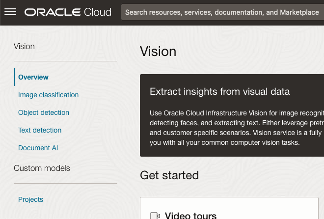
Open the OCI Vision page. On the bottom left-hand side of the menu you will see Projects. Click on this to open the Projects page for creating a Custom AI Vision model.
On the Create Projects page, click on the Create Project button. A pop-up window will appear. Enter the name for the model and click on the Create Project bottom at the bottom of the pop-up.
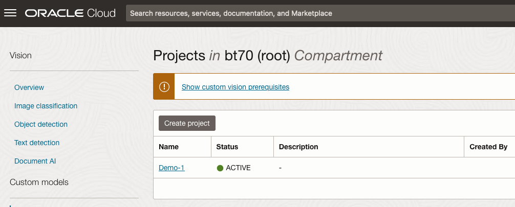
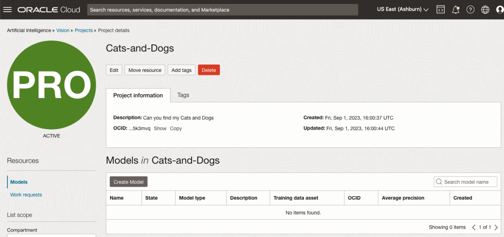
After the Project has been created, click on the project name from the list. This will open the Project specific page. A project can contain multiple models and they will be listed here. For the Cats-and-Dogs project we and to create our model. Click on the Create Model button.
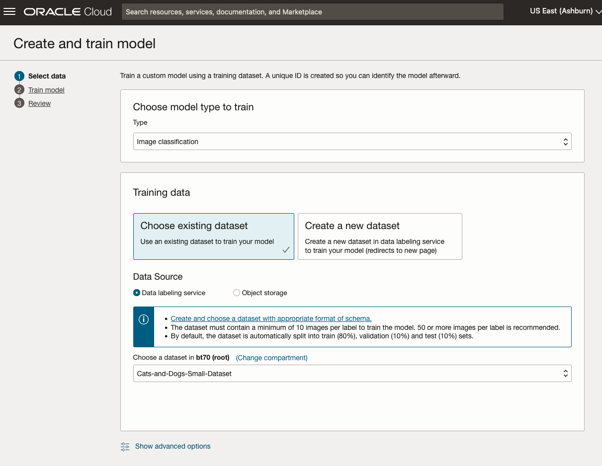
Next, you can define some of the settings for the Model. These include what dataset to use, or upload a new one, define what data labelling to use and the training duration. For this later setting, you can decide how much time you’d like to allocate to creating the custom model. Maybe consider selecting Quick mode, as that will give you a model within a few minutes (or up to an hour), whereas the other options can allow the model process to run for longer and hopefully those will create a more accurate model. As with all machine learning type models, you need to take some time to test which configuration works best for your scenario. In the following, the Quick mode option is selected. When read, click Create Model.

It can take a little bit of time to create the model. We selected the Quick mode, which has a maximum of one hour. In my scenario, the model build process was completed after four minutes. The Precentage Complete is updated during the build allowing you to monitor it’s progress.

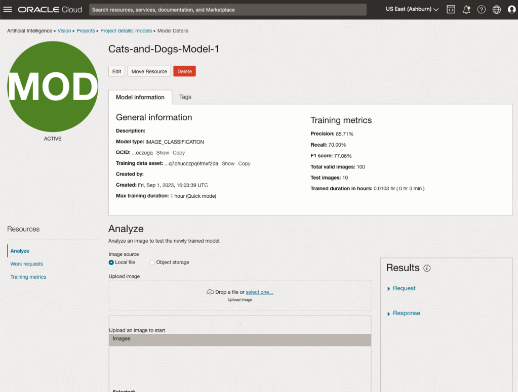
When the model is completed, you can test it using the Model page. Just click on the link for the model and you’ll get a page like the one to the right.
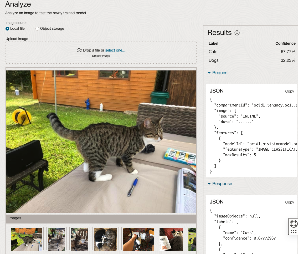
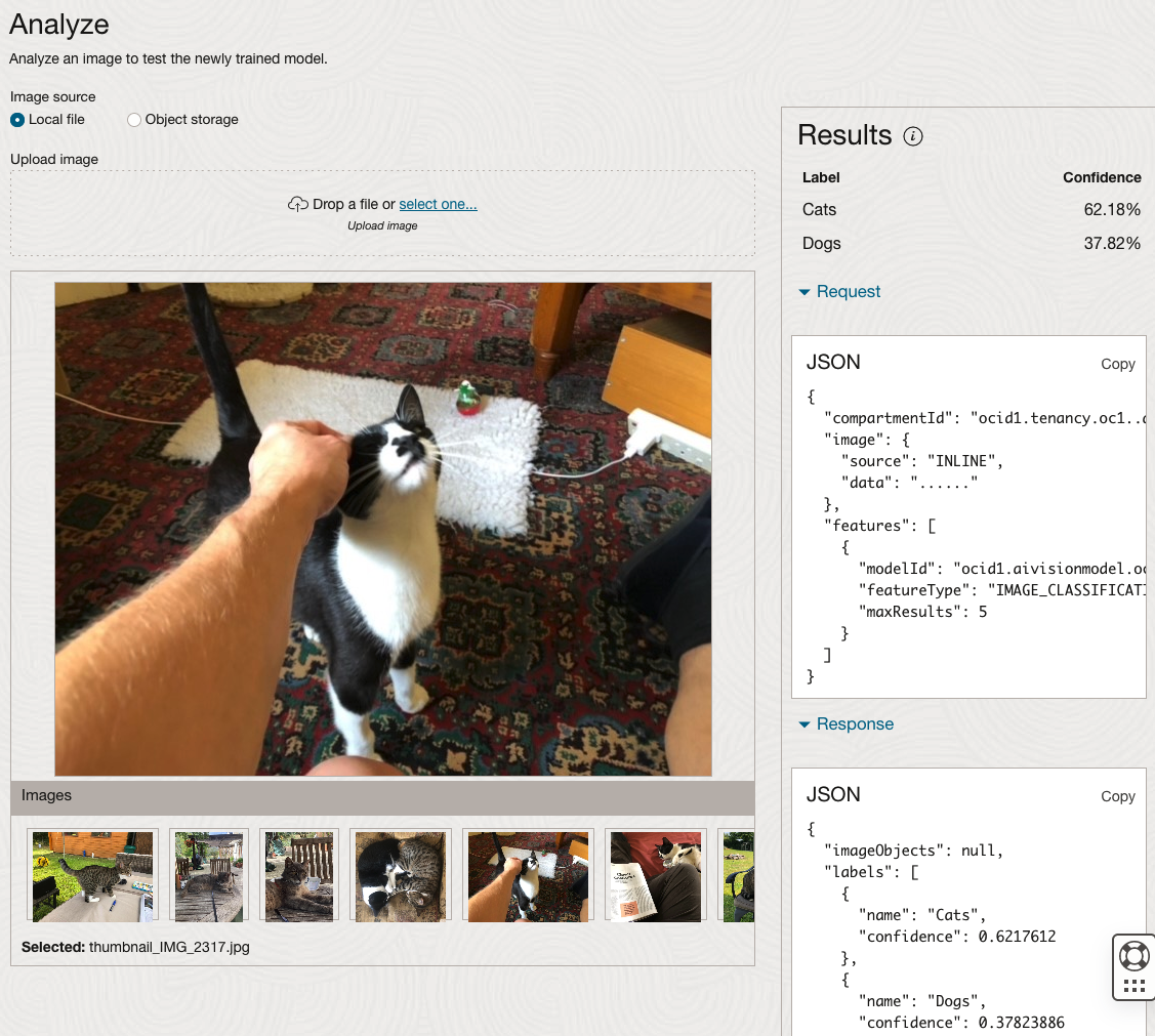
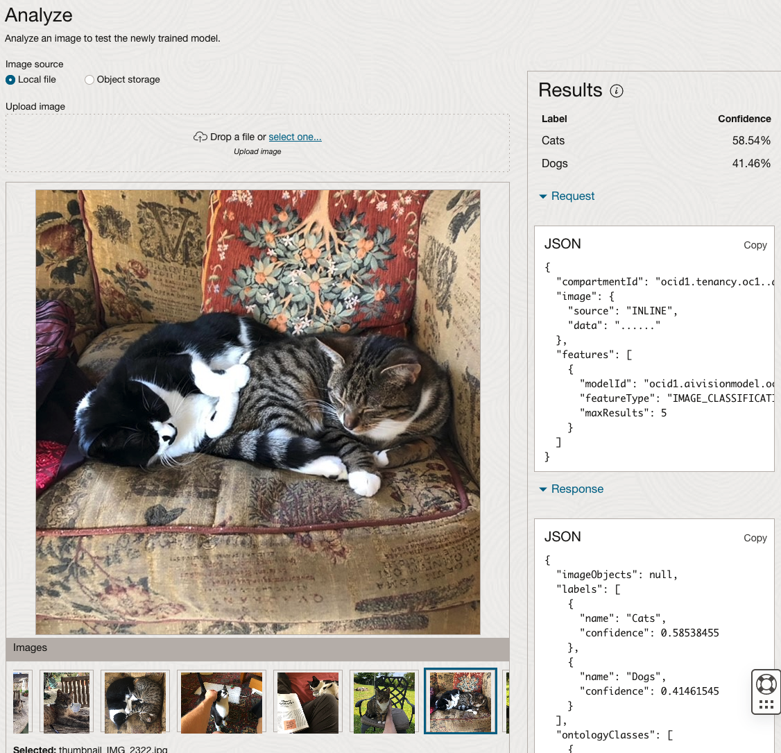
The bottom half of this page allows you to upload and evaluate images. The following images are example images of cats (do you know the owner) and the predictions and information about these are displayed on the screen. Have a look at the following to see which images scored better than others for identifying a Cat.
OCI Data Labeling for Machine Learning
OCI Data Labeling is a service that enables developers and data scientists to construct labelled datasets for training AI and machine learning models. By utilizing OCI Data Labeling, users can easily gather data, generate datasets, and assign labels to individual data records through user-friendly interfaces and public APIs. The labelled datasets can then be utilised to facilitate model development across a wide range of Oracle’s AI and data science services, ensuring a seamless and efficient model-building experience.
OCI Data Labeling allows developers and data scientists to label different types of data for training AI and machine learning models. Here are some examples of how OCI Data Labeling can be used for different types of data:
- Document Labeling
- Image Labeling
- Text Labeling
Typically the labelling of data is a manual task but there are also options to programmicly do this if the necessary label data is available.

The OCI Data Labeling service can be located under the Analytics & AI menu. See the image.
As we want to label a dataset, we need to first define the Dataset we want to use.
Select Datasets from the menu.
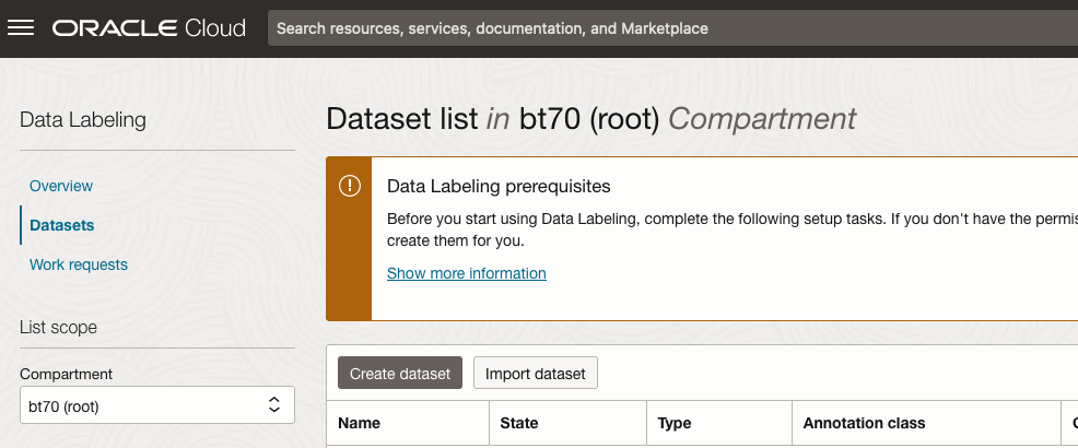
There are two options for creating the data set for labeling. The first is to use the Create Dataset option and the second is to Import Dataset.
If you already have your data in a Bucket, you can use both approaches. If you have a new dataset to import then use the Create Dataset option.
In this post, I’ll use the Create Dataset option and step through it.
Start by giving a name to the Dataset, then specify the type of data (Images, Text or Documents). In this example, we will work with image data.
Then select if the dataset (or each image) has one or multiple labels, or if you are going to draw bounding boxes for Object Detection.
For our example, select Single Label.
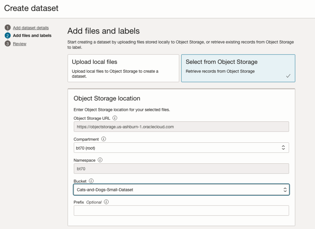
You can upload files from your computer or use files in an Object Bucket. As the dataset has already been loaded into a Bucket, we’ll select that option.
The Object Storage URL, Compartment and Namespace will be automatically populated for you.
Select the Bucket you want to use from the drop-down list. This dataset has 50 images each of Cats and Dogs.
The page will display the first eight or so, of the images in the Bucket. You can scroll through the others and this gives you a visual opportunity to make sure you are using the correct dataset.
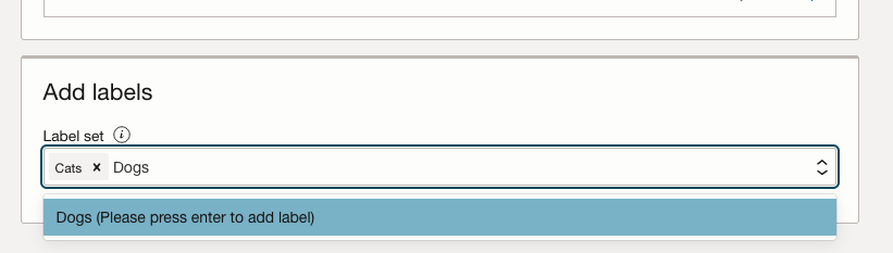
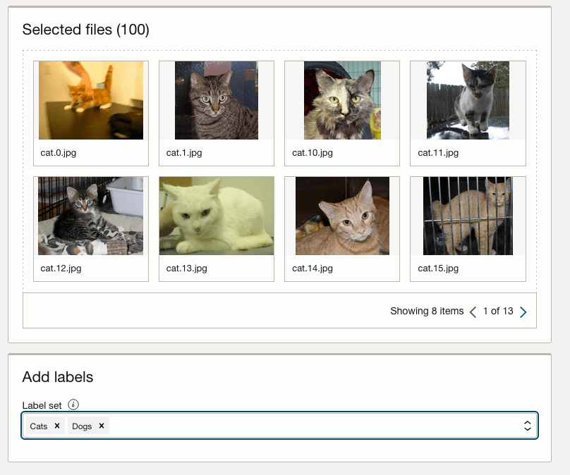
Now you can define the Labels to use for the dataset. In our sample dataset we only have two possible labels. If your dataset has more than this just enter the name and present enter. The Lable will be created.
You can add and remove labels.
When finished click the Next button at the bottom of the screen.
The final part of this initial setup is to create the dataset by clicking on the Create button
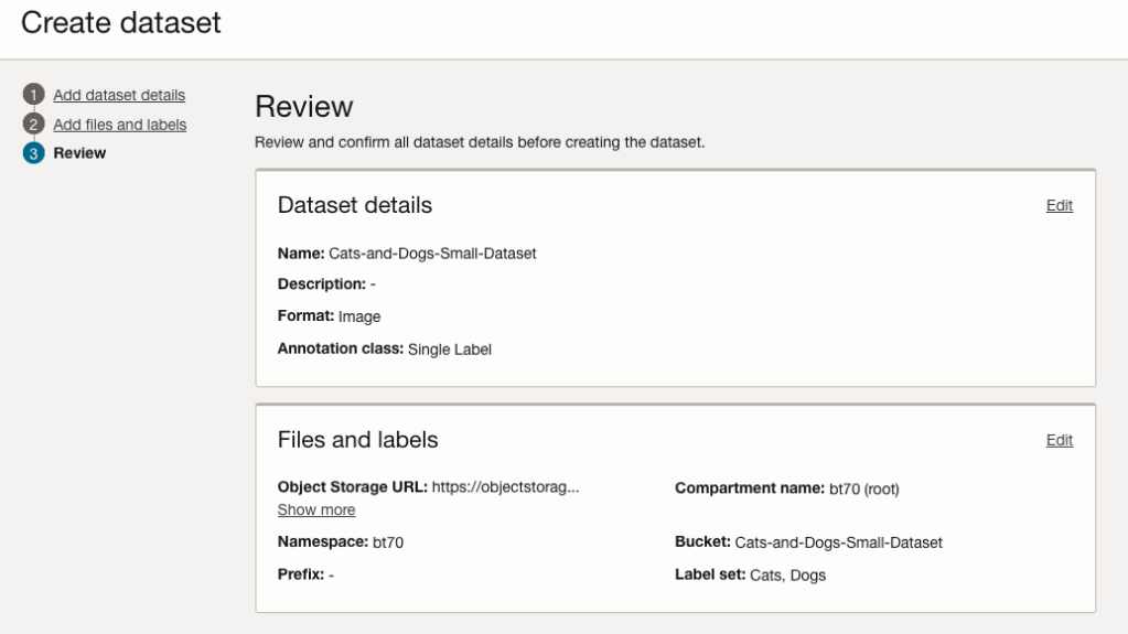
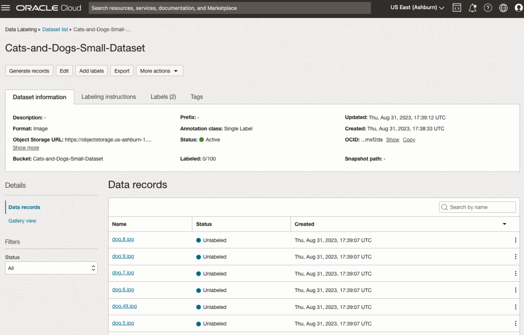
When everything has been processed you will get a screen that looks like this.
You are now ready to move on to labelling the dataset.
To label each image, start by clicking on the first image. This will open a screen like what is shown (to the right).
Click on the radio group item for the label that best represents the image. In some scenarios maybe both labels are suitable, and in such cases just pick the most suitable one. In this example, I’ve selected Dog. An alternative approach is to use the bounding box labelling. I’ll have a different post illustrating that.
Select the most suitable label and then click ‘Save & next’ button.
Yes, you’ll need to do this for all the images in the dataset. Yes, this can take a lot of time, particularly if you have 100s, or 1000s of images. The Datasets screen has details of how many images have been labelled and or not, and you can easily search for unlabelled files and continue labelling, if you need to take a break.
OCI Object Storage Buckets
We can upload and store data in Object Storage on OCI. This allows us to load and store data in a variety of different formats and sizes. With this data/files in object storage, it can be easily accessed from an Oracle Database (e.g. Autonomous Database) and any other service on OCI. This allows building more complete business solutions in a more integrated way.
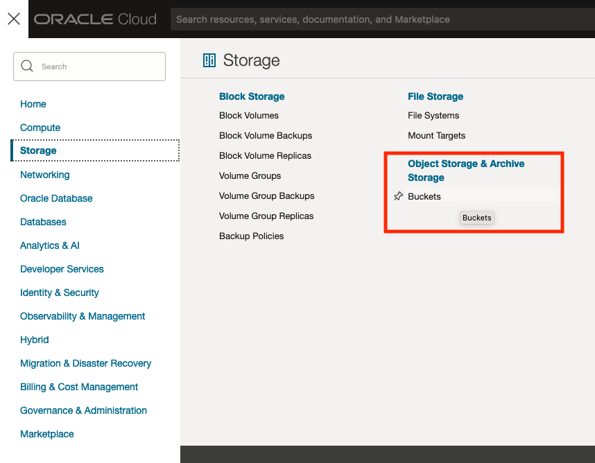
The Buckets feature can be found under the Storage option in the main Menu. From the popup screen look under Object Storage & Archive Storage and click on Buckets.
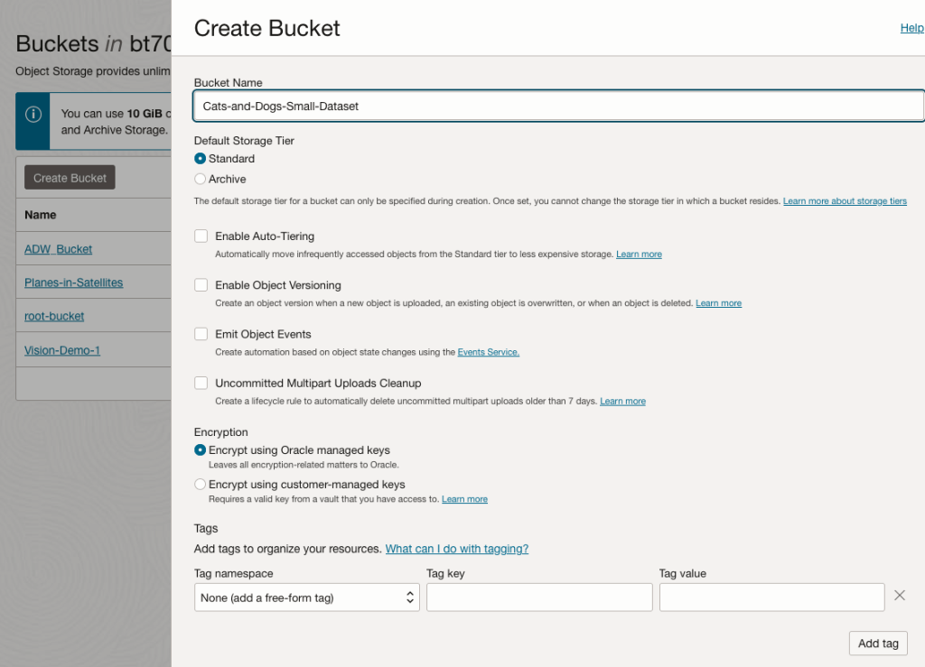
In the Objects Storage screen click on Create Bucket button.
In the Create Bucket screen, change the name of the Bucket. In this example, I’ve called it ‘Cats-and-Dogs-Small-Dataset’. No spaces are allowed. You can leave the defaults for the other settings. Then click the Create button.
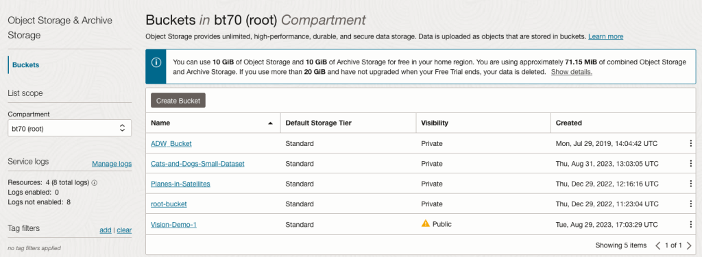
It will then be displayed along with any other buckets you have. I’ve a few other buckets.
Click on the Bucket name to open the bucket and add files to it.
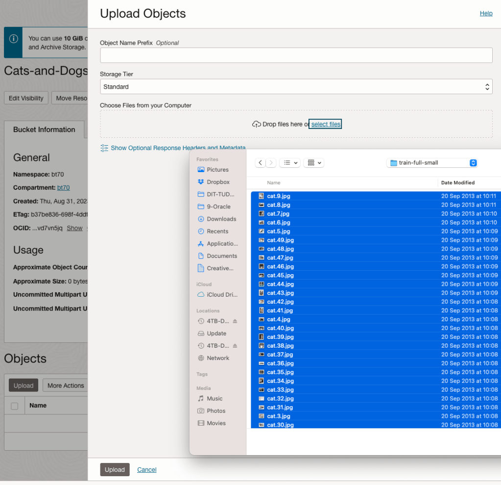
Click on the Upload button. Locate the files on your computer, select the files you want to upload.
The files will be listed in the Upload Object window. Click the Upload button to start transferring them to OCI.
If you wish you can set a prefix for all the files being uploaded.
When the files have been uploaded, click the Close button.
Note: The larger the dateset, in files and file size, it can take some time (depending on interest connection speed) for all the files to load into the Bucket.
To view the details of an image, click on the three dots to the right of the image files. This will open a menu for the image, where you can select to view image Details, download, copy, rename, delete, etc. the image.
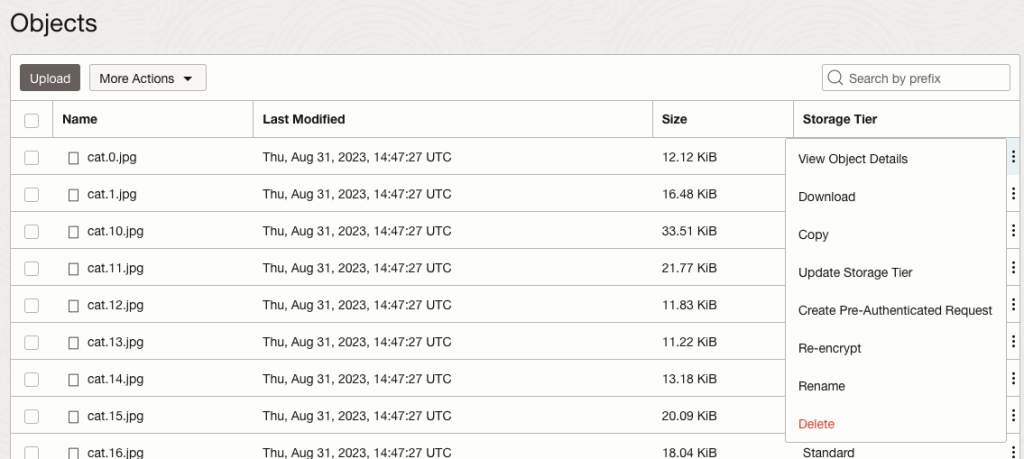

Click on View Object Details to get the details of the image.
This will display details about the object and the URI for the image.
OCI:Vision – AI for image processing – the Basics
Every cloud service provides some form of AI offering. Some of these can range from very basic features right up to a mediocre level. Only a few are delivering advanced AI services in a useful way.
Oracle AI Services have been around for about a year now, and with all new products or cloud services, a little time is needed to let it develop from an MVP (minimum viable produce) to something that’s more mature, feature-rich, stable and reliable. Oracle’s OCI AI Services come with some pre-training models and to create your own custom models based on your own training datasets.
Oracle’s OCI AI Services include:
- Digital Assistant
- Language
- Speech
- Vision
- Document Understand
- Anomaly Detection
- Forecasting
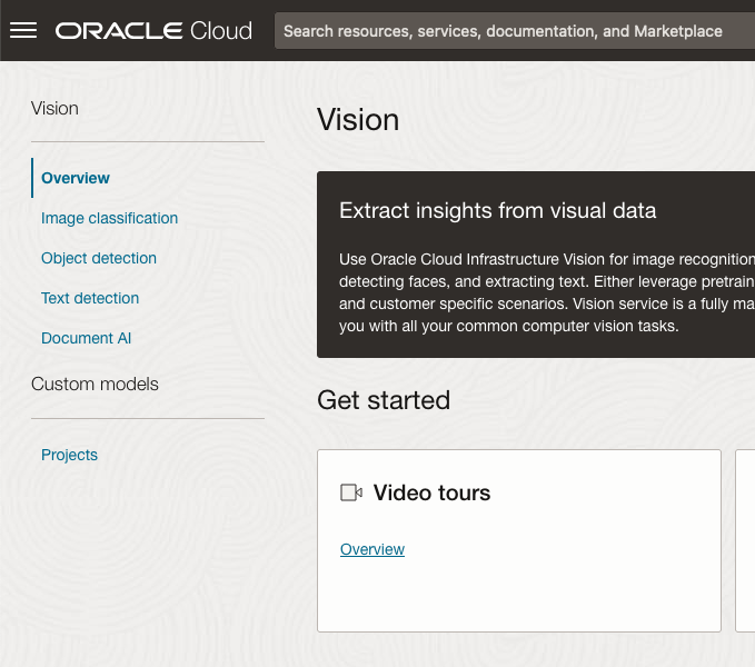
In this post, we’ll explore OCI Vision, and what the capabilities are available with their pre-trained models. To demonstrate this their online/webpage application will be used to demonstrate what it does and what it creates and identifies. You can access the Vision AI Services from the menu as shown in the following image.
From the main AI Vision webpage, we can see on the menu (on left-hand side of the page), we have three main Vision related options. These are Image Classification, Object Detection and Document AI. These are pre-trained models that perform slightly different tasks.
Let’s start with Image Classification and explore what is possible. Just Click on the link.
Note: The Document AI feature will be moving to its own cloud Service in 2024, so it will disappear from them many but will appear as a new service on the main Analytics & AI webpage (shown above).
The webpage for each Vision feature comes with a couple of images for you to examine to see how it works. But a better way to explore the capabilities of each feature is to use your own images or images you have downloaded. Here are examples.
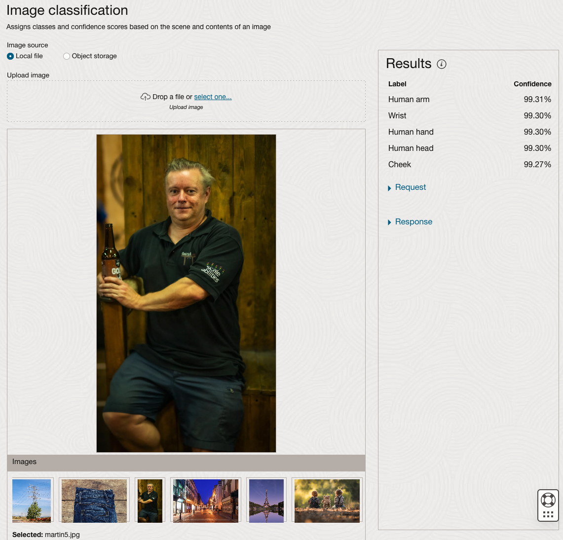
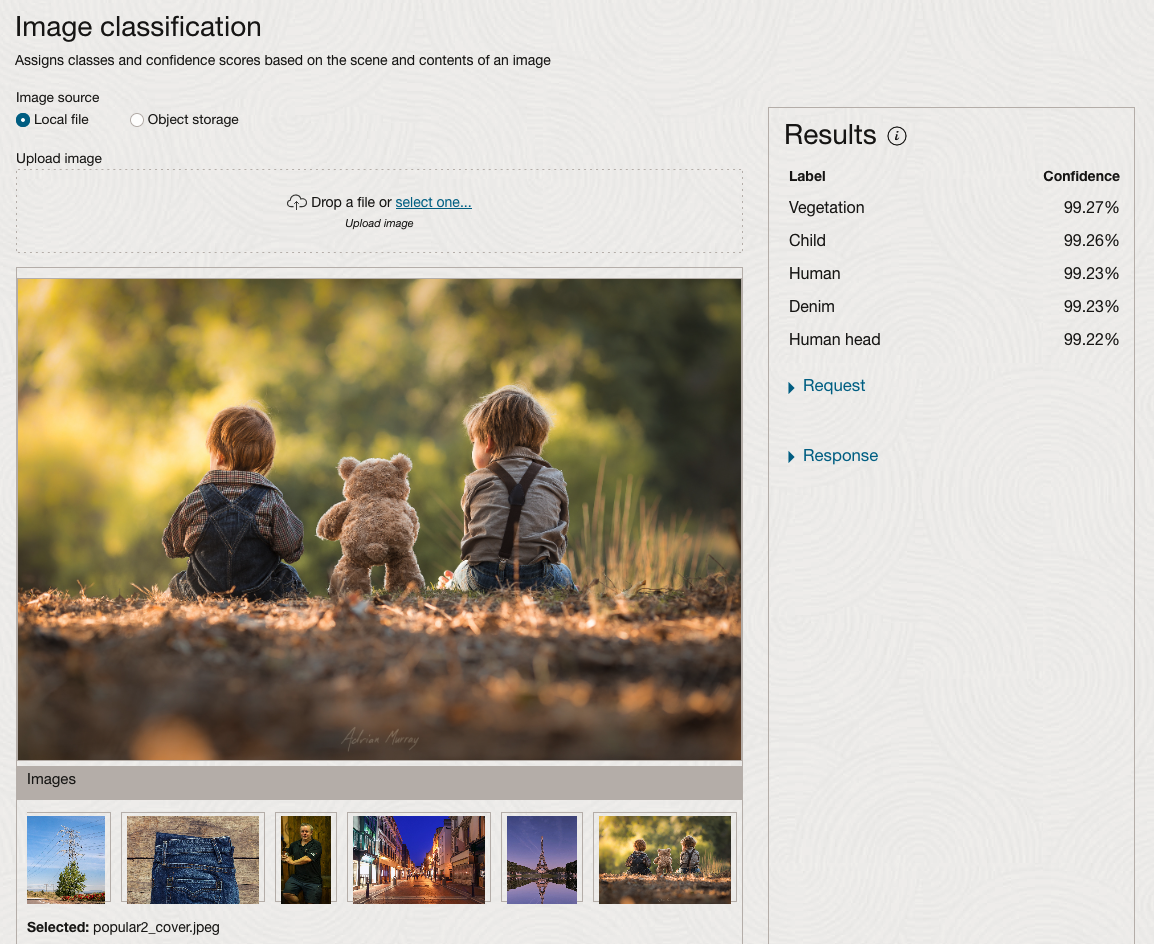
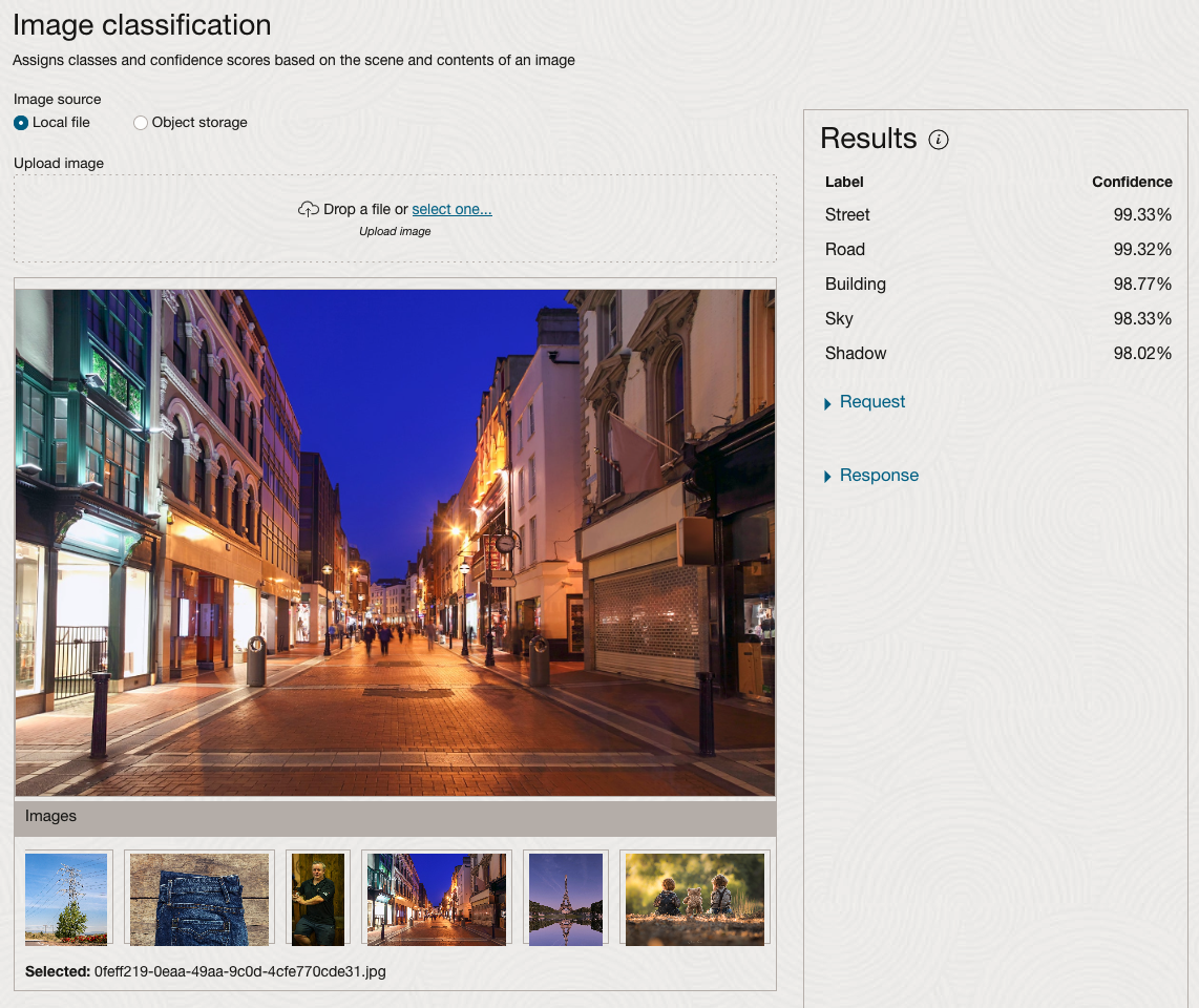
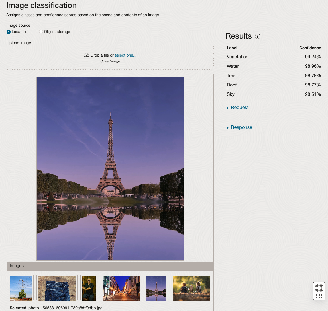
We can see the pre-trained model assigns classes and confidence for each image based on the main components it has identified in the image. For example with the Eiffel Tower image, the model has identified Water, Trees, Sky, Vegetation and Roof (of build). But it didn’t do so well with identifying the main object in the image as being a tower, or building of some form. Where with the streetscape image it was able to identify Street, Road, Building, Sky and Shadow.
Just under the Result section, we see two labels that can be expanded. One of these is the Response which contains JSON structure containing the labels, and confidences it has identified. This is what the pre-trained model returns and if you were to use Python to call this pre-trained model, it is this JSON object that you will get returned. You can then use the information contained in the JSON object to perform additional tasks for the image.
As you can see the webpage for OCI Vision and other AI services gives you a very simple introduction to what is possible, but it over simplifies the task and a lot of work is needed outside of this page to make the use of these pre-trained models useful.
Moving onto the Object Detection feature (left-hand menu) and using the pre-trained model on the same images, we get slightly different results.
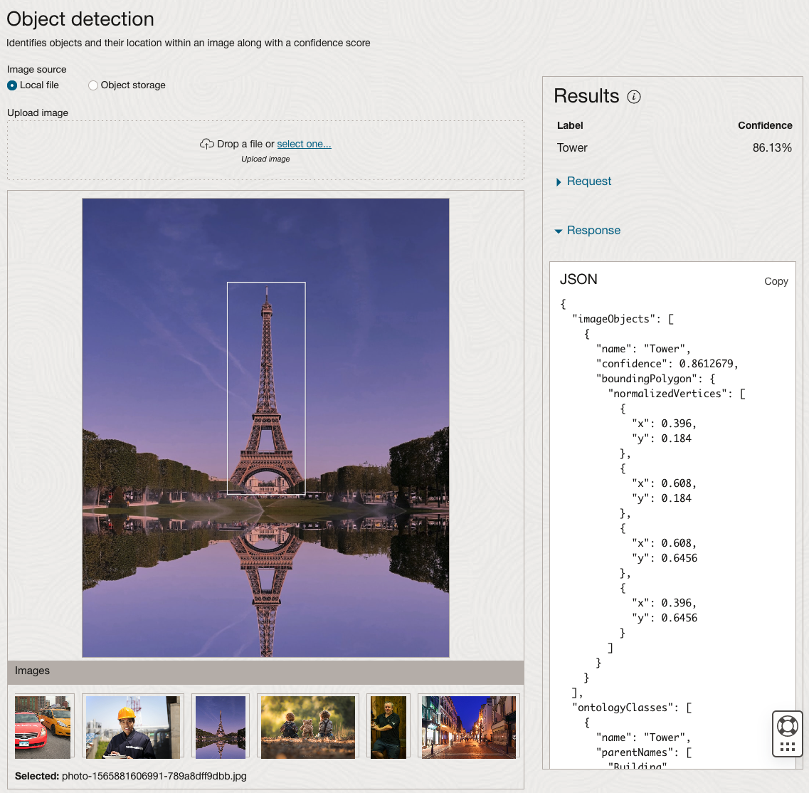
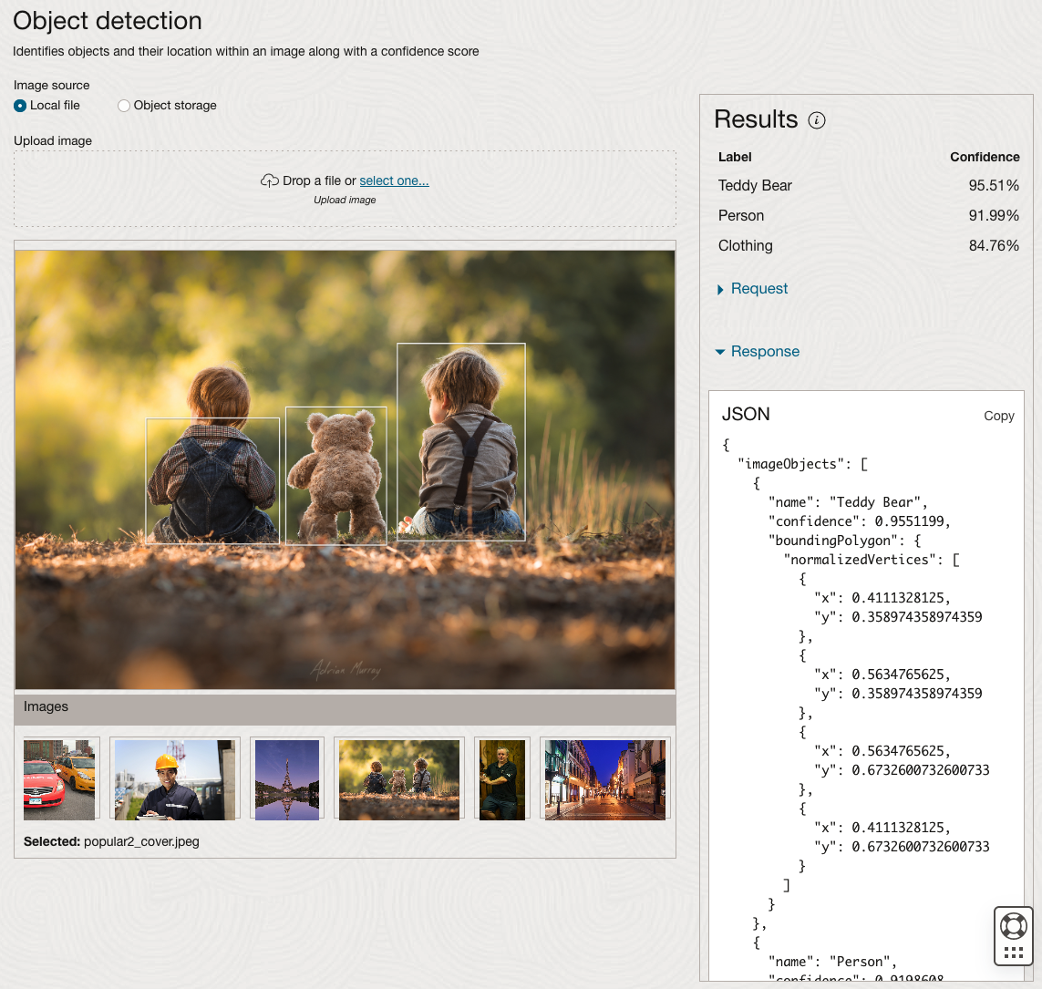
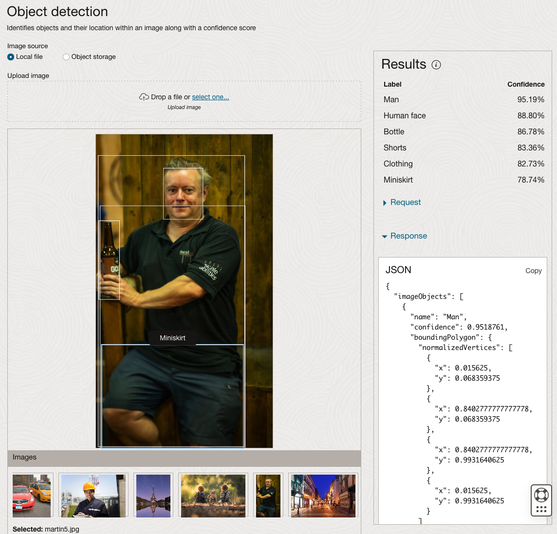
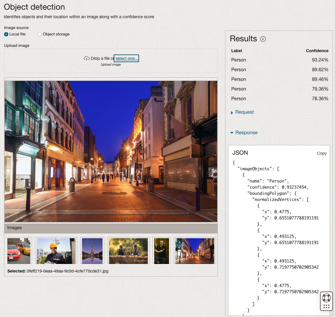
The object detection pre-trained model works differently as it can identify different things in the image. For example, with the Eiffel Tower image, it identifies a Tower in the image. In a similar way to the previous example, the model returns a JSON object with the label and also provides the coordinates for a bounding box for the objects detected. In the street scape image, it has identified five people. You’ll probably identify many more but the model identified five. Have a look at the other images and see what it has identified for each.
As I mentioned above, using these pre-trained models are kind of interesting, but are of limited use and do not really demonstrate the full capabilities of what is possible. Look out of additional post which will demonstrate this and steps needed to create and use your own custom model.
CAO Points 2023 – Slight Deflation
There have been lots of talk and news articles written about Grade Inflation over the past few years (the Covid years) and this year was no different. Most of the discussion this year began a couple of days before the Leaving Cert results were released last week and continued right up to the CAO publishing the points needed for each course. Yes, something needs to be done about the grading profiles and to revert back to pre-Covid levels. There are many reasons why this is necessary. Perhaps the most important of which is to bring back some stability to the Leaving Cert results and corresponding CAOs Points for entry to University courses. Last year, we saw there was some minor stepping back or deflating of results. But this didn’t have much of an impact on points needed for University courses. But in 2023 we have seen a slight step back in the points needed. I mentioned this possibility in my post on the Leaving Cert profile of marks. I also mentioned the subject with the biggest step back in marks/grades was Maths, and it looks like this has had an impact on the CAO point needed.
In 2023, we have seen a drop in points for 60% of University courses. In most years (pre and post-Covid) there would always be some fluctuation of points but the fluctuations would be minor. In 2023, some courses have changed by 20+ points.
The following table and chart illustrate the profile of CAO points and the percentage of students who achieved this in ranges of 50 points.
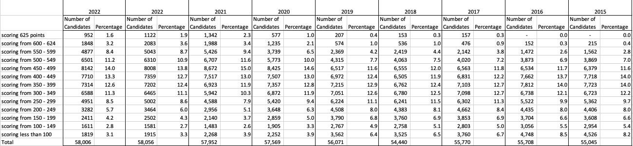

An initial look at the data and the chart it appears the 2023 CAO points profile is very similar to that of 2022. But when you look a little closer a few things stand out. At the upper end of CAO points we see a small reduction in the percentage of students. This is reflected when you look at the range of University courses in this range. The points for these have reduced slightly in 2023 and we have fewer courses using random selection. If you now look at the 300-500 range, we see a slight increase in the percentage of students attaining these marks. But this doesn’t seem to reflect an increase in the points needed to gain entry to a course in that range. This could be due to additional places that Universities have made available across the board. Although there are some courses where there is an increase.
In 2023, we have seen a change in the geographic spread of interest in University courses, with more demand/interest in Universities outside of the Dublin region. The lack of accommodation and their costs in Dublin is a major issue, and students have been looking elsewhere to study and to locations they can easily commute to. Although demand for Trinity and UCD remains strong, there was a drop in the number for TU Dublin. There are many reported factors for this which include the accommodation issue and for those who might have considered commuting, the positioning of the Grangegorman campus in Dublin does not make this easy, unlike Trinity, UCD and DCU.
I’ve the Leaving Cert grades by subject and CAO Points datasets in a Database (Oracle). This allows me to easily analyse the data annually and to compare them to previous years, using a variety of tools.
OCI:Vision Template for Policies
When using OCI you’ll need to configure your account and other users to have the necessary privileges and permissions to run the various offerings. OCI Vision is no different. You have two options for doing this. The first is to manually configure these. There isn’t a lot to do but some issues can arise. The other option is to use a template. The OCI Vision team have created a template of what is required and I’ll walk through the steps of setting this up along with some additional steps you’ll need.
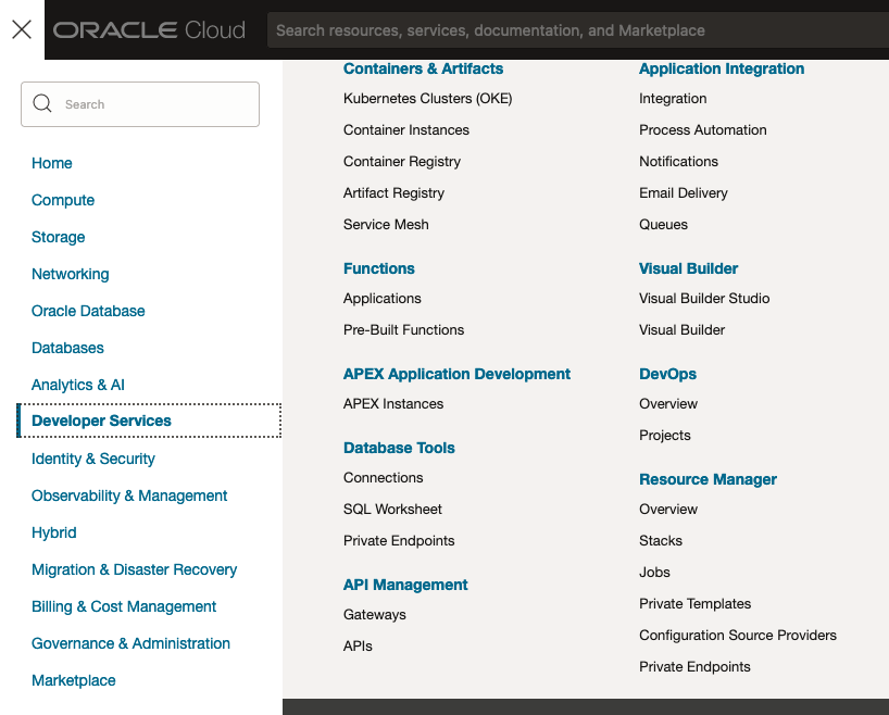
You’ll need to go to the Resource Manager page. This can be found under the menu by going to the Developer Services and then selecting Resource Manager.
First, you’ll need to go to the Resource Manager page. This can be found under the menu by going to the Developer Services and then selecting Resource Manager.
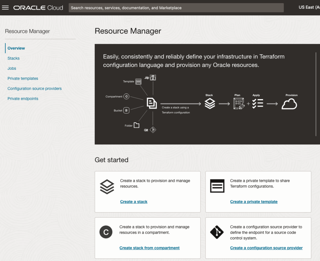
Located just under the main banner image you’ll see a section labelled ‘Create a stack’. Click on this link.
In the Create stack screen select Template from the radio group at the top of the page. Then in the Browse template pop-up screen, select the Service tab (across the top) and locate Vision. Once selected click the Select Template button.
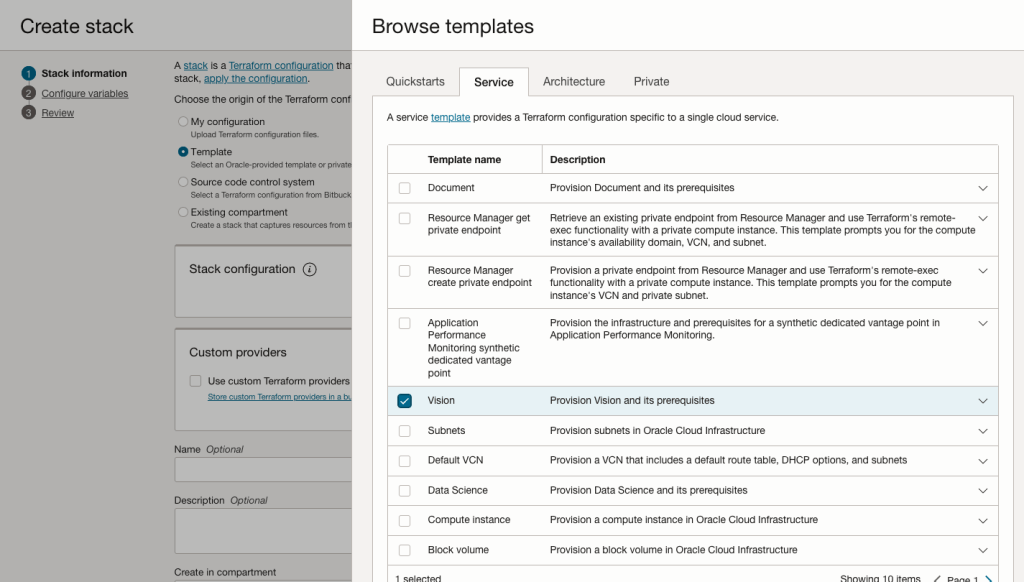
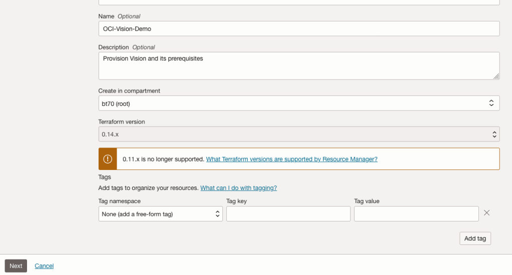
The page will load the necessary configuration. The only other thing you need to change on this page is the Name of the Service. Make it meaningful for you and your project. Click the Next button to continue to the next screen.
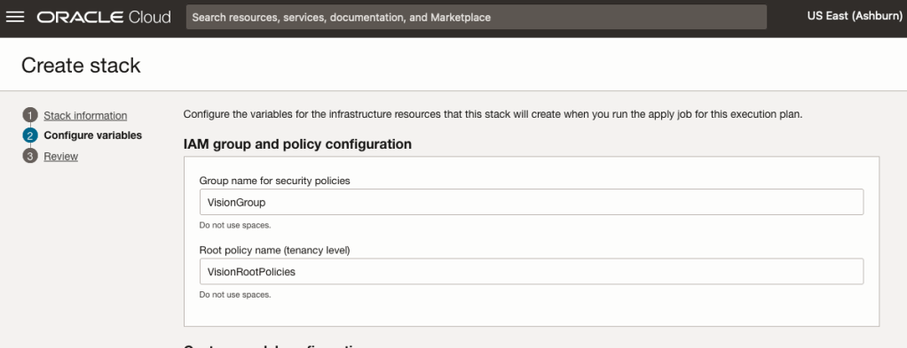
The top section relates to IAM Group name and policy configuration. You take the defaults or if you have specific groups already configured you can change it to it.
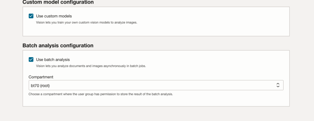
Most people will want to create their own customer models, as the supplied pre-built models are a bit basic. To enable Custom Built models, just tick the checkbox in the Custom Model Configuration section.
The second checkbox enables the batch processing of documents/images. If you check this box, you’ll need to specify the compartment you want the workload to be assigned to. Then click the Next button.
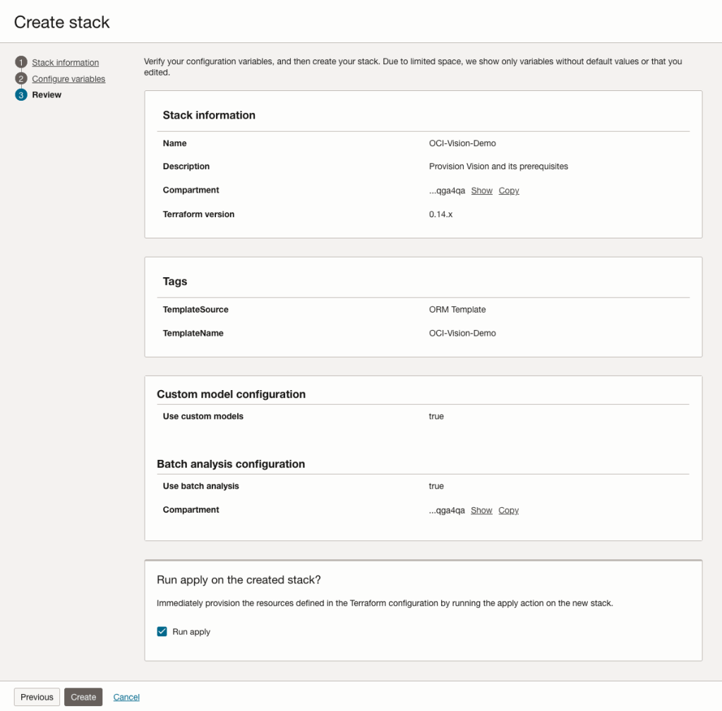
The final part displays a verification page of what was selected in the previous steps.
When ready click on the Run Apply check box and then click on the Create button.
It can take anything from a few seconds or a couple of minutes for the scripts to run.
When completed you’ll a Green box at the top of the screen and the message ‘SUCCEEDED’ under it.

Leaving Certificate 2023: In-line or more adjustments
The Leaving Certificate results were released this morning. Congratulations to everyone who has completed this major milestone. It’s a difficult set of examinations and despite all the calls to reform the examinations process, it has largely remained unchanged in decades, apart from some minor changes.
Last year (2022) I analysed some of the Leaving Certificate results. This was primarily focused on higher level papers and for a subset of the subjects. Some of these are the core subjects and some of the optional subjects. Just like last year we are told by the Department of Education the results this year will in-aggregate be in-line with last year. This statement is very confusing and also misleading. What does it really mean? No one has given a clear definition or explanation. What it tries to convey is the profile marks by subject are the same as last year. We say last year this was Not the case and we saw some grade deflation back towards the pre-Covid profile. Some though a similar stepping back this year, just like we have seen in the UK and other European countries.
The State Examinations Commission has released the break down of numbers and percentages of student who were awarded each grade by students. There are lots of ways to analyse this data from using Python and other Data Analytics tools, but for me I’ve loaded the data into an Oracle Database, and used Oracle Analytics Cloud to do some of the analysis along with other tools.
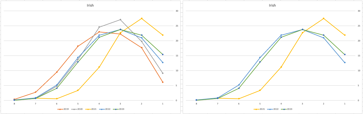
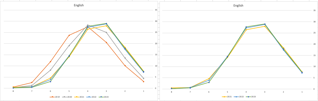
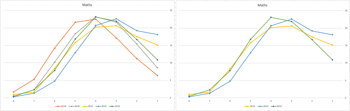
Let’s start with the core exam subjects of Irish, English and Maths. For Irish, last year we saw a step back in the profile of marks. This was a significant step back towards the marks in 2019 (pre-Covid). There wasn’t much discussion about this last year, and perhaps one of the reason is Irish is typically not counted towards their CAO points, as it is typically one of the weaker subjects for a lot of students. This year the profile of marks for Irish is in-line with last year’s profile (+/- small percentages) with slight up tick in H1 grades. For English, the profile of marks for 2021, 2022 and 2023 are almost exactly the same. But for Maths we do see a step back (moving the the left in the figure below) with a significantly lower percentage of student achieving a H2 or H1. Although we do see a slight increase in those getting H4 and H3 grades There was some problems with one of the Maths papers and perhaps marks were not adjusted due to those issues, which isn’t right to me as something should have been done. But perhaps a decision was made to all this step back in Maths to reduce the number of students achieving the top points of 625 and avoiding the scenario where those student do not get their first choice course for university.
The SEC have said the following about the marking of Maths Paper 1. “This process resulted in a marking scheme that was at the more lenient end of the normal range“. Even with more lenient marking and grade adjustments the profile of marks has taken a step backwards. This does raise question about how lenient they were or no and if the post mark adjusts took into account last year’s profile, or they are looking to step back to pre-Covid profiles.
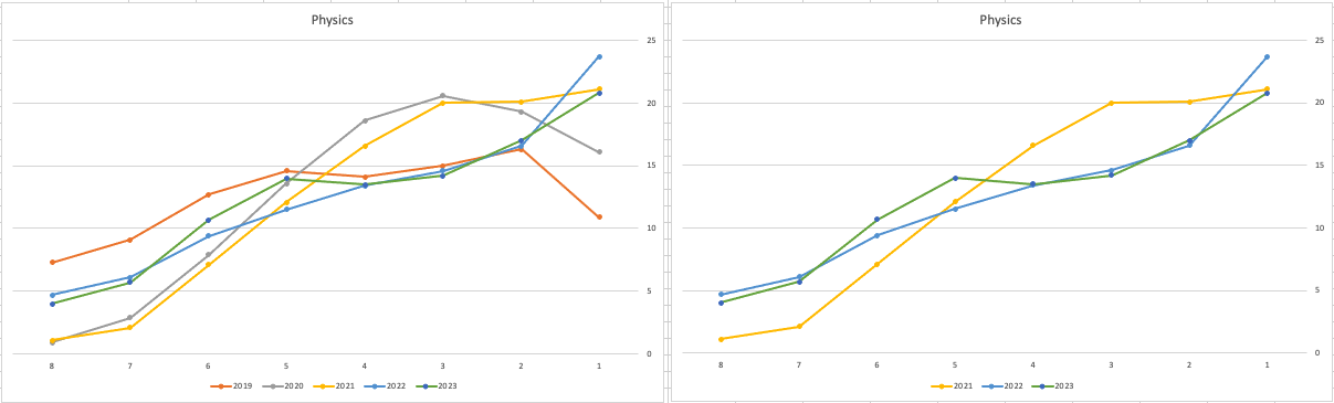
When we look at the Science students of Physics, Chemistry and Biology, we can see the profile of marks for this year is broadly in line with last years (2022). When looking at the profiles for these subjects, we can see that they are very similar to the pre-Covid profiles. Although there are some minor differences. We are still seeing an increased level H1s across this students when compared to pre-Covid 2019 levels. With lower grades having a slightly smaller percentage profile when compared to pre-Covid 2019 level. Look at the profiles 2022 and 2023 are broadly in-line with with 2019 (with some minor variations).
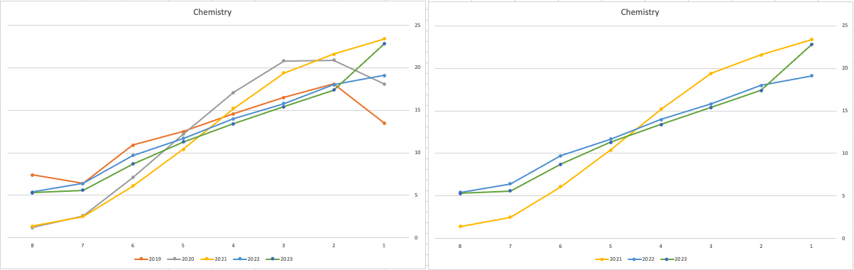
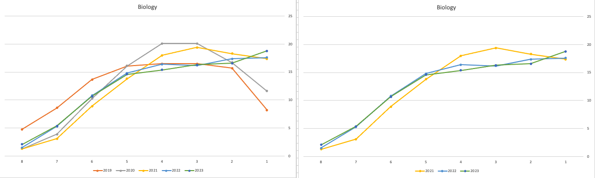
There are more subjects to report upon, but those listed above will cover most students.
What do these results and profile of marks mean for students looking to go to University or further education where the courses are based on the CAO Points systems. It looks like the step back in grade profile for Maths will have the biggest impact on CAO Points for courses. This will particularly impact those courses in the 525-625 range in 2022. We could see a small drop in marks for courses in that range with a possible drop of up to 10 points for some of those courses.
For courses in the 400-520 range in 2022, we might see a small increase in marks. Again this might be due to the profile of marks in Maths, but also with some of the other optional subjects. This year we could see a slight increase of 5-15 points for those courses.
Time will tell if these predictions come true, and hopefully every student will get the course they are hoping for as the nervous wait for CAO Round 1 offers commece. (Wednesday 30th August). I’ll have another post looking at the CAO Points profiles, so look out for that.
SQL:2023 Standard
As of June 2023 the new standard for SQL had been released, by the International Organization for Standards. Although SQL language has been around since the 1970s, this is the 11th release or update to the SQL standard. The first version of the standard was back in 1986 and the base-level standard for all databases was released in 1992 and referred to as SQL-92. That’s more than 30 years ago, and some databases still don’t contain all the base features in that standard, although they aim to achieve this sometime in the future.
| Year | Name | Alias | New Features or Enhancements |
|---|---|---|---|
| 1996 | SQL-86 | SQL-87 | This is the first version of the SQL standard by ANSI. Transactions, CREATE, Read, Update and Delete |
| 1989 | SQL-89 | This version includes minor revisions that added integrity constraints. | |
| 1992 | SQL-92 | SQL2 | This version includes major revisions on the SQL Language. Considered the base version of SQL. Many database systems, including NoSQL databases, use this standard for the base specification language, with varying degrees of implementation. |
| 1999 | SQL:1999 | SQL3 | This version introduces many new features such as regex matching, triggers, object-oriented features, OLAP capabilities and User Defined Types. The BOOLEAN data type was introduced but it took some time for all the major databases to support it. |
| 2003 | SQL:2003 | This version contained minor modifications to SQL:1999. SQL:2003 introduces new features such as window functions, columns with auto-generated values, identity specification and the addition of XML. | |
| 2006 | SQL:2006 | This version defines ways of importing, storing and manipulating XML data. Use of XQuery to query data in XML format. | |
| 2008 | SQL:2008 | This version includes major revisions to the SQL Language. Considered the base version of SQL. Many database systems, including NoSQL databases, use this standard for the base specification language, with varying degrees of implementation. | |
| 2011 | SQL:2011 | This version adds enhancements for window functions and FETCH clause, and Temporal data | |
| 2016 | SQL:2016 | This version adds various functions to work with JSON data and Polymorphic Table functions. | |
| 2019 | SQL:2019 | This version specifies muti-dimensional arrays data type. | |
| 2023 | SQL:2023 | This version contains minor updates to SQL functions to bring them in-line with how databases have implemented them. New JSON updates to include a new JSON data type with simpler dot notation processing. The main new addition to the standard is Property Graph Query (PDQ) which defines ways for the SQL language to represent property graphs and to interact with them. |
The Property Graph Query (PGQ) new features have been added as a new section or part of the standard and can be found labelled as Part-16: Property Graph Queries (SQL/PGQ). You can purchase the document for €191. Or you can read and scroll through the preview here.
For the other SQL updates, these updates were to reflect how the various (mainstream) database vendors (PostgreSQL, MySQL, Oracle, SQL Server, have implemented various functions. The standard is catching up with what is happening across the industry. This can be seen in some of the earlier releases
The following blog posts give a good overview of the SQL changes in the SQL:2023 standard.
Although SQL:2023 has been released there are some discussions about the next release of the standard. Although SQL:PGQ has been introduced, it also looks like (from various reports), some parts of SQL:PGQ were dropped and not included. More work is needed on these elements and will be included in the next release.
Also for the next release, there will be more JSON functionality included, with a particular focus on JSON Schemas. Yes, you read that correctly. There is a realisation that a schema is a good thing and when JSON objects can consist of up to 80% meta-data, a schema will have significant benefits for storage, retrieval and processing.
They are also looking at how to incorporate Streaming data. We can see some examples of this kind of processing in other languages and tools (Spark SQL, etc)
The SQL Standard is still being actively developed and we should see another update in a few years time.
Oracle 23c DBMS_SEARCH – Ubiquitous Search
One of the new PL/SQL packages with Oracle 23c is DBMS_SEARCH. This can be used for indexing (and searching) multiple schema objects in a single index.
Check out the documentation for DBMS_SEARCH.
This type of index is a little different to your traditional index. With DBMS_SEARCH we can create an index across multiple schema objects using just a single index. This gives us greater indexing capabilities for scenarios where we need to search data across multiple objects. You can create a ubiquitous search index on multiple columns of a table or multiple columns from different tables in a given schema. All done using one index, rather than having to use multiples. Because of this wider search capability, you will see this (DBMS_SEARCH) being referred to as a Ubiquitous Search Index. A ubiquitous search index is a JSON search index and can be used for full-text and range-based searches.
To create the index, you will first define the name of the index, and then add the different schema objects (tables, views) to it. The main commands for creating the index are:
- DBMS_SEARCH.CREATE_INDEX
- DBMS_SEARCH.ADD_SOURCE
Note: Each table used in the ADD_SOURCE must have a primary key.
The following is an example of using this type of index using the HR schema/data set.
exec dbms_search.create_index('HR_INDEX');This just creates the index header.
Important: For each index created using this method it will create a table with the Index name in your schemas. It will also create fourteen DR$ tables in your schema. SQL Developer filtering will help to hide these and minimise the clutter.
select table_name from user_tables;
...
HR_INDEX
DR$HR_INDEX$I
DR$HR_INDEX$K
DR$HR_INDEX$N
DR$HR_INDEX$U
DR$HR_INDEX$Q
DR$HR_INDEX$C
DR$HR_INDEX$B
DR$HR_INDEX$SN
DR$HR_INDEX$SV
DR$HR_INDEX$ST
DR$HR_INDEX$G
DR$HR_INDEX$DG
DR$HR_INDEX$KG
To add the contents and search space to the index we need to use ADD_SOURCE. In the following, I’m adding two tables to the index.
exec DBMS_SEARCH.ADD_SOURCE('HR_INDEX', 'EMPLOYEES');NOTE: At the time of writing this post some of the client tools and libraries do not support the JSON datatype fully. If they did, you could just query the index metadata, but until such time all tools and libraries fully support the data type, you will need to use the JSON_SERIALIZE function to translate the metadata. If you query the metadata and get no data returned, then try using this function to get the data.
Running a simple select from the index might give you an error due to the JSON type not being fully implemented in the client software. (This will change with time)
select * from HR_INDEX;But if we do a count from the index, we could get the number of objects it contains.
select count(*) from HR_INDEX;
   COUNT(*)
___________
        107
We can view what data is indexed by viewing the virtual document.
select json_serialize(DBMS_SEARCH.GET_DOCUMENT('HR_INDEX',METADATA))
from HR_INDEX;

JSON_SERIALIZE(DBMS_SEARCH.GET_DOCUMENT('HR_INDEX',METADATA))
___________________________________________________________________________________________________________________________________________________________________________________________________________________________________________________________________________
{"HR":{"EMPLOYEES":{"PHONE_NUMBER":"515.123.4567","JOB_ID":"AD_PRES","SALARY":24000,"COMMISSION_PCT":null,"FIRST_NAME":"Steven","EMPLOYEE_ID":100,"EMAIL":"SKING","LAST_NAME":"King","MANAGER_ID":null,"DEPARTMENT_ID":90,"HIRE_DATE":"2003-06-17T00:00:00"}}}
{"HR":{"EMPLOYEES":{"PHONE_NUMBER":"515.123.4568","JOB_ID":"AD_VP","SALARY":17000,"COMMISSION_PCT":null,"FIRST_NAME":"Neena","EMPLOYEE_ID":101,"EMAIL":"NKOCHHAR","LAST_NAME":"Kochhar","MANAGER_ID":100,"DEPARTMENT_ID":90,"HIRE_DATE":"2005-09-21T00:00:00"}}}
{"HR":{"EMPLOYEES":{"PHONE_NUMBER":"515.123.4569","JOB_ID":"AD_VP","SALARY":17000,"COMMISSION_PCT":null,"FIRST_NAME":"Lex","EMPLOYEE_ID":102,"EMAIL":"LDEHAAN","LAST_NAME":"De Haan","MANAGER_ID":100,"DEPARTMENT_ID":90,"HIRE_DATE":"2001-01-13T00:00:00"}}}
{"HR":{"EMPLOYEES":{"PHONE_NUMBER":"590.423.4567","JOB_ID":"IT_PROG","SALARY":9000,"COMMISSION_PCT":null,"FIRST_NAME":"Alexander","EMPLOYEE_ID":103,"EMAIL":"AHUNOLD","LAST_NAME":"Hunold","MANAGER_ID":102,"DEPARTMENT_ID":60,"HIRE_DATE":"2006-01-03T00:00:00"}}}
{"HR":{"EMPLOYEES":{"PHONE_NUMBER":"590.423.4568","JOB_ID":"IT_PROG","SALARY":6000,"COMMISSION_PCT":null,"FIRST_NAME":"Bruce","EMPLOYEE_ID":104,"EMAIL":"BERNST","LAST_NAME":"Ernst","MANAGER_ID":103,"DEPARTMENT_ID":60,"HIRE_DATE":"2007-05-21T00:00:00"}}}
We can search the metadata for certain data using the CONTAINS or JSON_TEXTCONTAINS functions.
select json_serialize(metadata)
from DEMO_IDX
where contains(data, 'winston')>0;
select json_serialize(metadata)
from DEMO_IDX
where json_textcontains(data, '$.HR.EMPLOYEES.FIRST_NAME', 'Winston');When the index is no longer required it can be dropped by running the following. Don’t run a DROP INDEX command as that removes some objects and leaves others behind! (leaves a bit of mess) and you won’t be able to recreate the index, unless you give it a different name.
exec dbms_search.drop_index('SH_INDEX');
You must be logged in to post a comment.