
Python
#GE2020 Analysing Party Manifestos using Python
The general election is underway here in Ireland with polling day set for Saturday 8th February. All the politicians are out campaigning and every day the various parties are looking for publicity on whatever the popular topic is for that day. Each day is it a different topic.
Most of the political parties have not released their manifestos for the #GE2020 election (as of date of this post). I want to use some simple Python code to perform some analyse of their manifestos. As their new manifestos weren’t available (yet) I went looking for their manifestos from the previous general election. Michael Pidgeon has a website with party manifestos dating back to the early 1970s, and also has some from earlier elections. Check out his website.
I decided to look at manifestos from the 4 main political parties from the 2016 general election. Yes there are other manifestos available, and you can use the Python code, given below to analyse those, with only some minor edits required.
The end result of this simple analyse is a WordCloud showing the most commonly used words in their manifestos. This is graphical way to see what some of the main themes and emphasis are for each party, and also allows us to see some commonality between the parties.
Let’s begin with the Python code.
1 – Initial Setup
There are a number of Python Libraries available for processing PDF files. Not all of them worked on all of the Part Manifestos PDFs! It kind of depends on how these files were generated. In my case I used the pdfminer library, as it worked with all four manifestos. The common library PyPDF2 didn’t work with the Fine Gael manifesto document.
import io
import pdfminer
from pprint import pprint
from pdfminer.converter import TextConverter
from pdfminer.pdfinterp import PDFPageInterpreter
from pdfminer.pdfinterp import PDFResourceManager
from pdfminer.pdfpage import PDFPage

#directory were manifestos are located
wkDir = '.../General_Election_Ire/'

#define the names of the Manifesto PDF files & setup party flag
pdfFile = wkDir+'FGManifesto16_2.pdf'
party = 'FG'
#pdfFile = wkDir+'Fianna_Fail_GE_2016.pdf'
#party = 'FF'
#pdfFile = wkDir+'Labour_GE_2016.pdf'
#party = 'LB'
#pdfFile = wkDir+'Sinn_Fein_GE_2016.pdf'
#party = 'SF'
All of the following code will run for a given manifesto. Just comment in or out the manifesto you are interested in. The WordClouds for each are given below.
2 – Load the PDF File into Python
The following code loops through each page in the PDF file and extracts the text from that page.
I added some addition code to ignore pages containing the Irish Language. The Sinn Fein Manifesto contained a number of pages which were the Irish equivalent of the preceding pages in English. I didn’t want to have a mixture of languages in the final output.
SF_IrishPages = [14,15,16,17,18,19,20,21,22,23,24]
text = ""

pageCounter = 0
resource_manager = PDFResourceManager()
fake_file_handle = io.StringIO()
converter = TextConverter(resource_manager, fake_file_handle)
page_interpreter = PDFPageInterpreter(resource_manager, converter)

for page in PDFPage.get_pages(open(pdfFile,'rb'), caching=True, check_extractable=True):
    if (party == 'SF') and (pageCounter in SF_IrishPages):
        print(party+' - Not extracting page - Irish page', pageCounter)
    else:
        print(party+' - Extracting Page text', pageCounter)
        page_interpreter.process_page(page)

        text = fake_file_handle.getvalue()

    pageCounter += 1

print('Finished processing PDF document')
converter.close()
fake_file_handle.close()
FG - Extracting Page text 0
FG - Extracting Page text 1
FG - Extracting Page text 2
FG - Extracting Page text 3
FG - Extracting Page text 4
FG - Extracting Page text 5
...
3 – Tokenize the Words
The next step is to Tokenize the text. This breaks the text into individual words.
from nltk.tokenize import word_tokenize
from nltk.corpus import stopwords
tokens = []

tokens = word_tokenize(text)

print('Number of Pages =', pageCounter)
print('Number of Tokens =',len(tokens))
Number of Pages = 140
Number of Tokens = 66975
4 – Filter words, Remove Numbers & Punctuation
There will be a lot of things in the text that we don’t want included in the analyse. We want the text to only contain words. The following extracts the words and ignores numbers, punctuation, etc.
#converts to lower case, and removes punctuation and numbers
wordsFiltered = [tokens.lower() for tokens in tokens if tokens.isalpha()]
print(len(wordsFiltered))
print(wordsFiltered)
58198
['fine', 'gael', 'general', 'election', 'manifesto', 's', 'keep', 'the', 'recovery', 'going', 'gaelgeneral', 'election', 'manifesto', 'foreward', 'from', 'an', 'taoiseach', 'the', 'long', 'term', 'economic', 'three', 'steps', 'to', 'keep', 'the', 'recovery', 'going', 'agriculture', 'and', 'food', 'generational',
...
As you can see the number of tokens has reduced from 66,975 to 58,198.
5 – Setup Stop Words
Stop words are general words in a language that doesn’t contain any meanings and these can be removed from the data set. Python NLTK comes with a set of stop words defined for most languages.
#We initialize the stopwords variable which is a list of words like
#"The", "I", "and", etc. that don't hold much value as keywords
stop_words = stopwords.words('english')
print(stop_words)
['i', 'me', 'my', 'myself', 'we', 'our', 'ours', 'ourselves', 'you', "you're", "you've", "you'll", "you'd", 'your', 'yours', 'yourself',
....
Additional stop words can be added to this list. I added the words listed below. Some of these you might expect to be in the stop word list, others are to remove certain words that appeared in the various manifestos that don’t have a lot of meaning. I also added the name of the parties and some Irish words to the stop words list.
#some extra stop words are needed after examining the data and word cloud
#these are added
extra_stop_words = ['ireland','irish','ł','need', 'also', 'set', 'within', 'use', 'order', 'would', 'year', 'per', 'time', 'place', 'must', 'years', 'much', 'take','make','making','manifesto','ð','u','part','needs','next','keep','election', 'fine','gael', 'gaelgeneral', 'fianna', 'fáil','fail','labour', 'sinn', 'fein','féin','atá','go','le','ar','agus','na','ár','ag','haghaidh','téarnamh','bplean','page','two','number','cothromfor']
stop_words.extend(extra_stop_words)
print(stop_words)
Now remove these stop words from the list of tokens.
# remove stop words from tokenised data set
filtered_words = [word for word in wordsFiltered if word not in stop_words]
print(len(filtered_words))
print(filtered_words)
31038
['general', 'recovery', 'going', 'foreward', 'taoiseach', 'long', 'term', 'economic', 'three', 'steps', 'recovery', 'going', 'agriculture', 'food',
The number of tokens is reduced to 31,038
6 – Word Frequency Counts
Now calculate how frequently these words occur in the list of tokens.
#get the frequency of each word
from collections import Counter

# count frequencies
cnt = Counter()
for word in filtered_words:
cnt[word] += 1

print(cnt)
Counter({'new': 340, 'support': 249, 'work': 190, 'public': 186, 'government': 177, 'ensure': 177, 'plan': 176, 'continue': 168, 'local': 150,
...
7 – WordCloud
We can use the word frequency counts to add emphasis to the WordCloud. The more frequently it occurs the larger it will appear in the WordCloud.
#create a word cloud using frequencies for emphasis
from wordcloud import WordCloud
import matplotlib.pyplot as plt

wc = WordCloud(max_words=100, margin=9, background_color='white',
scale=3, relative_scaling = 0.5, width=500, height=400,
random_state=1).generate_from_frequencies(cnt)

plt.figure(figsize=(20,10))
plt.imshow(wc)
#plt.axis("off")
plt.show()

#Save the image in the img folder:
wc.to_file(wkDir+party+"_2016.png")
The last line of code saves the WordCloud image as a file in the directory where the manifestos are located.
8 – WordClouds for Each Party

Remember these WordClouds are for the manifestos from the 2016 general election.
When the parties have released their manifestos for the 2020 general election, I’ll run them through this code and produce the WordClouds for 2020. It will be interesting to see the differences between the 2016 and 2020 manifesto WordClouds.
Data Profiling in Python
With every data analytics and data science project, one of the first tasks to that everyone needs to do is to profile the data sets. Data profiling allows you to get an initial picture of the data set, see data distributions and relationships. Additionally it allows us to see what kind of data cleaning and data transformations are necessary.
Most data analytics tools and languages have some functionality available to help you. Particular the various data science/machine learning products have this functionality built-in them and can do a lot of the data profiling automatically for you. But if you don’t use these tools/products, then you are probably using R and/or Python to profile your data.
With Python you will be working with the data set loaded into a Pandas data frame. From there you will be using various statistical functions and graphing functions (and libraries) to create a data profile. From there you will probably create a data profile report.
But one of the challenges with doing this in Python is having different coding for handling numeric and character based attributes/features. The describe function in Python (similar to the summary function in R) gives some statistical summaries for numeric attributes/features. A different set of functions are needed for character based attributes. The Python Library repository (https://pypi.org/) contains over 200K projects. But which ones are really useful and will help with your data science projects. Especially with new projects and libraries being released on a continual basis? This is a major challenge to know what is new and useful.
For example the followings shows loading the titanic data set into a Pandas data frame, creating a subset and using the describe function in Python.
import pandas as pd

df = pd.read_csv("/Users/brendan.tierney/Dropbox/4-Datasets/titanic/train.csv")

df.head(5)

df2 = df.iloc[:,[1,2,4,5,6,7,8,10,11]]
df2.head(5)

df2.describe()

You will notice the describe function has only looked at the numeric attributes.
One of those 200+k Python libraries is one called pandas_profiling. This will create a data audit report for both numeric and character based attributes. This most be good, Right? Let’s take a look at what it does.
For each column the following statistics – if relevant for the column type – are presented in an interactive HTML report:
- Essentials: type, unique values, missing values
- Quantile statistics like minimum value, Q1, median, Q3, maximum, range, interquartile range
- Descriptive statistics like mean, mode, standard deviation, sum, median absolute deviation, coefficient of variation, kurtosis, skewness
- Most frequent values
- Histogram
- Correlations highlighting of highly correlated variables, Spearman, Pearson and Kendall matrices
- Missing values matrix, count, heatmap and dendrogram of missing values
The first step is to install the pandas_profiling library.
pandas-profiling package naming was changed. To continue profiling data use ydata-profiling instead!
pip3 install pandas_profiling
Now run the pandas_profiling report for same data frame created and used, see above.
import pandas_profiling as pp

df2.profile_report()
The following images show screen shots of each part of the report. Click and zoom into these to see more details.


Managing imbalanced Data Sets with SMOTE in Python
When working with data sets for machine learning, lots of these data sets and examples we see have approximately the same number of case records for each of the possible predicted values. In this kind of scenario we are trying to perform some kind of classification, where the machine learning model looks to build a model based on the input data set against a target variable. It is this target variable that contains the value to be predicted. In most cases this target variable (or feature) will contain binary values or equivalent in categorical form such as Yes and No, or A and B, etc or may contain a small number of other possible values (e.g. A, B, C, D).
For the classification algorithm to perform optimally and be able to predict the possible value for a new case record, it will need to see enough case records for each of the possible values. What this means, it would be good to have approximately the same number of records for each value (there are many ways to overcome this and these are outside the score of this post). But most data sets, and those that you will encounter in real life work scenarios, are never balanced, as in having a 50-50 split. What we typically encounter might be a 90-10, 98-2, etc type of split. These data sets are said to be imbalanced.

The image above gives examples of two approaches for creating a balanced data set. The first is under-sampling. This involves reducing the class that contains the majority of the case records and reducing it to match the number of case records in the minor class. The problems with this include, the resulting data set is too small to be meaningful, the case records removed could contain important records and scenarios that the model will need to know about.
The second example is creating a balanced data set by increasing the number of records in the minority class. There are a few approaches to creating this. The first approach is to create duplicate records, from the minor class, until such time as the number of case records are approximately the same for each class. This is the simplest approach. The second approach is to create synthetic records that are statistically equivalent of the original data set. A commonly technique used for this is called SMOTE, Synthetic Minority Oversampling Technique. SMOTE uses a nearest neighbors algorithm to generate new and synthetic data we can use for training our model. But one of the issues with SMOTE is that it will not create sample records outside the bounds of the original data set. As you can image this would be very difficult to do.
The following examples will illustrate how to perform Under-Sampling and Over-Sampling (duplication and using SMOTE) in Python using functions from Pandas, Imbalanced-Learn and Sci-Kit Learn libraries.
NOTE: The Imbalanced-Learn library (e.g. SMOTE)requires the data to be in numeric format, as it statistical calculations are performed on these. The python function get_dummies was used as a quick and simple to generate the numeric values. Although this is perhaps not the best method to use in a real project. With the other sampling functions can process data sets with a sting and numeric.
Data Set: Is the Portuaguese Banking data set and is available on the UCI Data Set Repository, and many other sites. Here are some basics with that data set.
import warnings

import pandas as pd
import numpy as np
import matplotlib.pyplot as plt
get_ipython().magic('matplotlib inline')

bank_file = ".../bank-additional-full.csv"

# import dataset
df = pd.read_csv(bank_file, sep=';',)

# get basic details of df (num records, num features)
df.shape
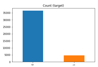
df['y'].value_counts() # dataset is imbalanced with majority of class label as "no".
no     36548
yes     4640
Name: y, dtype: int64
#print bar chart
df.y.value_counts().plot(kind='bar', title='Count (target)');
Example 1a – Down/Under sampling the majority class y=1 (using random sampling)
count_class_0, count_class_1 = df.y.value_counts()

# Divide by class
df_class_0 = df[df['y'] == 0] #majority class
df_class_1 = df[df['y'] == 1] #minority class

# Sample Majority class (y=0, to have same number of records as minority calls (y=1)
df_class_0_under = df_class_0.sample(count_class_1)
# join the dataframes containing y=1 and y=0
df_test_under = pd.concat([df_class_0_under, df_class_1])

print('Random under-sampling:')
print(df_test_under.y.value_counts())
print("Num records = ", df_test_under.shape[0])

df_test_under.y.value_counts().plot(kind='bar', title='Count (target)');

Example 1b – Down/Under sampling the majority class y=1 using imblearn
from imblearn.under_sampling import RandomUnderSampler

X = df_new.drop('y', axis=1)
Y = df_new['y']

rus = RandomUnderSampler(random_state=42, replacement=True)
X_rus, Y_rus = rus.fit_resample(X, Y)

df_rus = pd.concat([pd.DataFrame(X_rus), pd.DataFrame(Y_rus, columns=['y'])], axis=1)

print('imblearn over-sampling:')
print(df_rus.y.value_counts())
print("Num records = ", df_rus.shape[0])

df_rus.y.value_counts().plot(kind='bar', title='Count (target)');
[same results as Example 1a]
Example 1c – Down/Under sampling the majority class y=1 using Sci-Kit Learn
from sklearn.utils import resample

print("Original Data distribution")
print(df['y'].value_counts())

# Down Sample Majority class
down_sample = resample(df[df['y']==0],
replace = True, # sample with replacement
n_samples = df[df['y']==1].shape[0], # to match minority class
random_state=42) # reproducible results

# Combine majority class with upsampled minority class
train_downsample = pd.concat([df[df['y']==1], down_sample])

# Display new class counts
print('Sci-Kit Learn : resample : Down Sampled data set')
print(train_downsample['y'].value_counts())
print("Num records = ", train_downsample.shape[0])
train_downsample.y.value_counts().plot(kind='bar', title='Count (target)');
[same results as Example 1a]
Example 2 a – Over sampling the minority call y=0 (using random sampling)
df_class_1_over = df_class_1.sample(count_class_0, replace=True)
df_test_over = pd.concat([df_class_0, df_class_1_over], axis=0)

print('Random over-sampling:')
print(df_test_over.y.value_counts())

df_test_over.y.value_counts().plot(kind='bar', title='Count (target)');
Random over-sampling:
1    36548
0    36548
Name: y, dtype: int64

Example 2b – Over sampling the minority call y=0 using SMOTE
from imblearn.over_sampling import SMOTE

print(df_new.y.value_counts())
X = df_new.drop('y', axis=1)
Y = df_new['y']

sm = SMOTE(random_state=42)
X_res, Y_res = sm.fit_resample(X, Y)

df_smote_over = pd.concat([pd.DataFrame(X_res), pd.DataFrame(Y_res, columns=['y'])], axis=1)

print('SMOTE over-sampling:')
print(df_smote_over.y.value_counts())

df_smote_over.y.value_counts().plot(kind='bar', title='Count (target)');
[same results as Example 2a]
Example 2c – Over sampling the minority call y=0 using Sci-Kit Learn
from sklearn.utils import resample

print("Original Data distribution")
print(df['y'].value_counts())

# Upsample minority class
train_positive_upsample = resample(df[df['y']==1],
replace = True, # sample with replacement
n_samples = train_zero.shape[0], # to match majority class
random_state=42) # reproducible results

# Combine majority class with upsampled minority class
train_upsample = pd.concat([train_negative, train_positive_upsample])

# Display new class counts
print('Sci-Kit Learn : resample : Up Sampled data set')
print(train_upsample['y'].value_counts())
train_upsample.y.value_counts().plot(kind='bar', title='Count (target)');
[same results as Example 2a]
Migrating Python ML Models to other languages
I’ve mentioned in a previous blog post about experiencing some performance issues with using Python ML in production. We needed something quicker and the possible languages we considered were C, C++, Java and Go Lang.
But the data science team used R and Python, with just a few more people using Python than R on the team.
One option was to rewrite everything into the language used in production. As you can imagine no-one wanted to do that and there was no way of ensure a bug free solution and one that gave similar results to the R and Python models. The other option was to look for some code to convert the models from one language to another.
The R users was well versed in using PMML. Predictive Model Markup Language (PMML) has been around a long time and well known and used by certain groups of data scientists who have been around a while. It is also widely supported by many analytics vendors, and provides an inter-change format to allow predictive models to be described and exchanged. For newer people, they hadn’t heard of it. PMML is an XML based interchange specification.
But with PMML there are some limitation. Not with the specification but how it is implemented by the various vendors that support it. PMML supports the exchange of the model pipeline including the data transformations as well as the model specification. Most vendors only support some elements of this and maybe just a couple of models. And there-in lies the problem. How can a ML pipeline be migrated from, as Python, to some other language and/or tool. There are limitations.
If you do want to explore PMML with Python check out the sklearn2pmml package and is also available on PyPl. This package allows you to export the ML pipeline and the model specification. As with most other implementations of PMML there are some parts of the PMML specification not implement, but it is better than post of the other implementation out there.
An alternative is to look at code translations options. With these we want something that will take our ML pipeline and convert it to another programming language like C++, JAVA, Go, etc. There aren’t too many solutions available to do this. One such solution we’ve explored over the past couple of weeks is called m2cgen.
m2cgen (Model 2 Code Generator) is a lightweight library which provides an easy way to transpile trained statistical models into a native code (Python, C, Java, Go). You can supply M2cgen with a range of models (linear, SVM, tree, random forest, or boosting, etc) and the tool will output code in the chosen language that will represent the trained model. The code generated will generated into native code without dependencies. Other packages or libraries are not dependent or required in the translated language. For example here is an example Decision Tree translated into a number of different languages.
C
#include <string.h>
void score(double * input, double * output) {
    double var0[3];
    if ((input[2]) <= (2.6)) {
        memcpy(var0, (double[]){1.0, 0.0, 0.0}, 3 * sizeof(double));
    } else {
        if ((input[2]) <= (4.8500004)) {
            if ((input[3]) <= (1.6500001)) {
                memcpy(var0, (double[]){0.0, 1.0, 0.0}, 3 * sizeof(double));
            } else {
                memcpy(var0, (double[]){0.0, 0.3333333333333333, 0.6666666666666666}, 3 * sizeof(double));
            }
        } else {
            if ((input[3]) <= (1.75)) {
                memcpy(var0, (double[]){0.0, 0.42857142857142855, 0.5714285714285714}, 3 * sizeof(double));
            } else {
                memcpy(var0, (double[]){0.0, 0.0, 1.0}, 3 * sizeof(double));
            }
        }
    }
    memcpy(output, var0, 3 * sizeof(double));
}
Java
public class Model {

    public static double[] score(double[] input) {
        double[] var0;
        if ((input[2]) <= (2.6)) {
            var0 = new double[] {1.0, 0.0, 0.0};
        } else {
            if ((input[2]) <= (4.8500004)) {
                if ((input[3]) <= (1.6500001)) {
                    var0 = new double[] {0.0, 1.0, 0.0};
                } else {
                    var0 = new double[] {0.0, 0.3333333333333333, 0.6666666666666666};
                }
            } else {
                if ((input[3]) <= (1.75)) {
                    var0 = new double[] {0.0, 0.42857142857142855, 0.5714285714285714};
                } else {
                    var0 = new double[] {0.0, 0.0, 1.0};
                }
            }
        }
        return var0;
    }
}
Go Lang
func score(input []float64) []float64 {
    var var0 []float64
    if (input[2]) <= (2.6) {
        var0 = []float64{1.0, 0.0, 0.0}
    } else {
        if (input[2]) <= (4.8500004) {
            if (input[3]) <= (1.6500001) {
                var0 = []float64{0.0, 1.0, 0.0}
            } else {
                var0 = []float64{0.0, 0.3333333333333333, 0.6666666666666666}
            }
        } else {
            if (input[3]) <= (1.75) {
                var0 = []float64{0.0, 0.42857142857142855, 0.5714285714285714}
            } else {
                var0 = []float64{0.0, 0.0, 1.0}
            }
        }
    }
    return var0
}
Python transforming Categorical to Numeric
When preparing data for input to machine learning algorithms you may have to perform certain types of data preparation.
In most enterprise solutions all or most of these tasks are automated for you, but in many languages they aren’t. The enterprise solutions are about ‘automating the boring stuff’ so that you don’t have to worry about it and waste valuable time doing boring, repetitive things.
The following examples illustrates a number of ways to record categorical variables into numeric. There are a number of approaches available, and it is up to you to decide which one might work best for your problem, your data, etc.
Let’s begin by loading the data set to be used in these examples. It is a Video Games reviews data set.
# perform some Statistics on the items in a panda
import pandas as pd
import numpy as np
import matplotlib as plt
videoReview = pd.read_csv('/Users/brendan.tierney/Downloads/Video_Games_Sales_as_at_22_Dec_2016.csv')
videoReview.head(10)

What are the data types of each variable
videoReview.dtypes

We don’t want to work with all the data in these examples. We just want to concentrate on the categorical variables. Let’s us create a subset of the dataframe to contains these.
df = videoReview.select_dtypes(include=['object']).copy()
df.head(10)

Now do a little data clean up by removing NaN (nulls)
df.dropna(inplace=True)
df.isnull().sum()

df.describe()

The above image shows the number of unique values in each of the variables. We will use Platform, Genre and Rating for the variable example below.
Let us chart these variables.
#check the number of passengars for each variable
import seaborn as sb
import matplotlib.pyplot as plt

plt.rcParams['figure.figsize'] = 10, 8

sb.countplot(x='Platform',data=df, palette='hls')

sb.countplot(x='Genre',data=df, palette='hls')

sb.countplot(x='Rating',data=df, palette='hls')

1-One-hot Coding
The first approach is to use the commonly used one-hot coding method. This will take a categorical variable and create a set of new variables corresponding with each distinct value in the variable, and then populate it with a binary value to indicate the original value.
#apply one-hot-coding to all the categorical variables
# and create a new dataframe to store the results

df2 = pd.get_dummies(df)
df2.head(10)

As you can see we now have 8138 variables in the pandas dataframe!
That is a lot and may not be workable for you. You may need to look at some feature reduction methods to reduce the number of variables.
2-Find and Replace
In this example we will simple replace the values with defined values.
Let’s have a look at values in the Ratings variable and their frequencies.
df['Rating'].value_counts()

The last 4 values listed have very small number of occurrences.
We will group these into having one value/category
find_replace = {"Rating" : {"E": 1, "T": 2, "M": 3, "E10+": 4, "EC": 5, "K-A": 5, "RP": 5, "AO": 5}}
df.replace(find_replace, inplace=True)
df.head(10)

Now plot the newly generated rating values and their frequencies.
sb.countplot(x='Rating',data=df, palette='hls')

3 – Label encoding
With this technique where each distinct value in a categorical variable is converted to a number.
In this scenario you don’t get to pick the numeric value assigned to the value. It is system determined.
#let's check the data types again
df.dtypes

Our categorical variables are of ‘object’ data type. We need to convert to a category data type.
In this example ‘Platform’ as it has a large-ish number of values and we want a quick way of converting them we can illustrate this by creating a new variable.
df["Platform_Category"] = df["Platform"].astype('category')
df.dtypes

Now convert this new variable to numeric.
df["Platform_Category"] = df["Platform_Category"].cat.codes
df.head(20)

The number assigned to the Platform_Category variable is based on the alphabetical ordering of the values in the Platform variable. For example,
df.groupby("Platform")["Platform"].count()

4-Using SciKit-Learn transform
SciKit-Learn has a number of functions to help with data encodings. The first one we will look at is the ‘fit_transform’ function.
This will perform a similar task to what we have seen in a previous example
#Let's use the fit_tranforms function to encode the Genre variable
from sklearn.preprocessing import LabelEncoder

le_make = LabelEncoder()
df["Genre_Code"] = le_make.fit_transform(df["Genre"])
df[["Genre", "Genre_Code"]].head(10)

And we can see this comparison when we look at the frequency counts.
df.groupby("Genre_Code")["Genre_Code"].count()

df.head(10)

And now we can drop the Genre variable from the dataframe as it is no longer needed. BUT you will need to have recorded the mapping between the original Genre values and the numeric values for future reference.
df = df.drop('Genre', axis=1)
df.head(10)

5-Using SciKit-Learn LabelEndcoder
SciKit-Learn has a binary label encoder and it can be used in a similar way to the previous example and also similar to the ‘get_dummies’ function.
from sklearn.preprocessing import LabelBinarizer

lb_style = LabelBinarizer()
lb_results = lb_style.fit_transform(df["Rating"])
lb_df = pd.DataFrame(lb_results, columns=lb_style.classes_)
lb_df.head(10)

These can now be joined with the original dataframe or a with a subset of the original dataframe to form a new dataframe consisting of the required variables.
As you can see, from the following, there are several other data pre-processing functions available in SciKit-Learn.

Moving Average in SQL (and beyond)
A very common analytics technique for financial and other data is to calculate the moving average. This can allow you to see a different type of pattern in your data that may not is evident from examining the original data.
But how can we calculate the moving average in SQL?
Well, there isn’t a function to do it, but we can use the windowing feature of analytical SQL to do so. The following example was created in an Oracle Database but the same SQL (more or less) will work with most other SQL databases.
SELECT month,
       SUM(amount) AS month_amount,
       AVG(SUM(amount)) OVER
          (ORDER BY month ROWS BETWEEN 3 PRECEDING AND CURRENT ROW) AS moving_average
FROM  sales
GROUP BY month
ORDER BY month;
This gives us the following with the moving average calculated based on the current value and the three preceding values, if they exist.
    MONTH MONTH_AMOUNT MOVING_AVERAGE
---------- ------------ --------------
         1     58704.52       58704.52
         2      28289.3       43496.91
         3     20167.83       35720.55
         4      50082.9     39311.1375
         5     17212.66     28938.1725
         6     31128.92     29648.0775
         7     78299.47     44180.9875
         8     42869.64     42377.6725
         9     35299.22     46899.3125
        10     43028.38     49874.1775
        11     26053.46      36812.675
        12     20067.28      31112.085
In some analytic languages and databases, they have included a moving average function. For example using HiveMall on Hive we have.
SELECT moving_avg(x, 3) FROM (SELECT explode(array(1.0,2.0,3.0,4.0,5.0,6.0,7.0)) as x) series;If you are using Python, there is an inbuilt function in Pandas.
rolmean4 = timeseries.rolling(window = 4).mean()
Machine Learning Models in Python – How long does it take
We keep hearing from people about all the computing resources needed for machine learning. Sometimes it can put people off from trying it as they will think I don’t have those kind of resources.
This is another blog post in my series on ‘How long does it take to create a machine learning model?‘
Check out my previous blog post that used data sets containing 72K, 210K, 660K, 2M and 10M records.
- Creating Machine Learning Models in Oracle Cloud Database service
- Creating Machine Learning Models using Oracle Autonomous Data Warehouse (ADW)
There was some surprising results in those these.
In this test, I’ll be using Python and SciKitLearn package to create models using the same algorithms. There are a few things to keep in mind. Firstly, although they maybe based on the same algorithms, the actual implementation of them will be different in each environment (SQL vs Python).
With using Python for machine learning, one of the challenges we have is getting access to the data. Assuming the data lives in a Database then time is needed to extract that data to the local Python environment. Secondly, when using Python you will be using a computer with significantly less computing resources than a Database server. In this test I used my laptop (MacBook Pro). Thirdly, when extracting the data from the database, what method should be used.
I’ve addressed these below and the Oracle Database I used was the DBaaS I used in my first experiment. This is a Database hosted on Oracle Cloud.
Extracting Data to CSV File
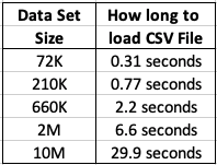
This kind of depends on how you do this. There are hundreds of possibilities available to you, but if you are working with an Oracle Database you will probably be using SQL Developer. I used the ‘export’ option to create a CSV file for each of the data sets. The following table shows how long it took for each data set.

As you can see this is an incredibly slow way of exporting this data. Like I said, there are quicker ways of doing this.
After downloading the data sets, the next step is to see how load it takes to load these CSV files into a pandas data frame in Python. The following table show the timings in seconds.
Extracting Data using cx_Oracle Python package
As I’ll be using Python to create the models and the data exists in an Oracle Database (on Oracle Cloud), I can use the cx_Oracle package to download the data sets into my Python environment. After using the cx_Oracle package to download the data I then converted it into a pandas data frame.
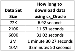
I had the array fetch size set to 10,000. I also experimented with smaller and larger numbers for the array fetch size, but 10,000 seemed to give a quickest results.
How long to create Machine Learning Models in Python
Now we get onto checking out the timings of how long it takes to create a number of machine learning models using different algorithms and using the default settings. The algorithms include Naive Bayes, Decision Tree, GLM, SVM and Neural Networks.
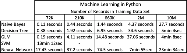
I had to stop including SVM in the tests as it was taking way too long to run. For example I killed the SVM model build on the 210K data set after it was running for 5 hours.
The Neural Network models created had 3 hidden layers.
In addition to creating the models, there was some minor data preparation steps performed including factorizing, normalization and one-hot-coding. This data preparation would be comparable to the automatic data preparation steps performed by Oracle, although Oracle Automatic Data Preparation does a bit of extra work.
At the point I would encourage you to look back at my previous blog posts on timings using Oracle DBaaS and ADW. You will see that Python, in these test cases, was quicker at creating the machine learning models. But with Python the data needed to be extracted from the database and that can take time!
A separate consideration is being able to deploy the models. The time it takes to build models is perhaps not the main consideration. You need to consider ease of deployment and use of the models.
RandomForests in R, Python and SQL
I recently wrote a two part article explaining how Random Forests work and how to use them in R, Python and SQL.
These were posted on ToadWorld webpages. Check them out.
Part 1 of article
https://blog.toadworld.com/2018/08/31/random-forest-machine-learning-in-r-python-and-sql-part-1
Part 2 of article
https://blog.toadworld.com/2018/09/01/random-forest-machine-learning-in-r-python-and-sql-part-2
R vs Python vs SQL for Machine Learning (Infographic)
Next week I’ll be giving several presentation on machine learning at Oracle Open World and Oracle Code One. In one of these presentation an evaluation of using R vs Python vs SQL will be given and discussed.
Check out the infographic containing the comparisons.

Twitter Analytics using Python – Part 2
This is my second (of five) post on using Python to process Twitter data.
Check out my all the posts in the series.
In this post I was going to look at two particular aspects. The first is the converting of Tweets to Pandas. This will allow you to do additional analysis of tweets. The second part of this post looks at how to setup and process streaming of tweets. The first part was longer than expected so I’m going to hold the second part for a later post.
Step 6 – Convert Tweets to Pandas
In my previous blog post I show you how to connect and download tweets. Sometimes you may want to convert these tweets into a structured format to allow you to do further analysis. A very popular way of analysing data is to us Pandas. Using Pandas to store your data is like having data stored in a spreadsheet, with columns and rows. There are also lots of analytic functions available to use with Pandas.
In my previous blog post I showed how you could extract tweets using the Twitter API and to do selective pulls using the Tweepy Python library. Now that we have these tweet how do I go about converting them into Pandas for additional analysis? But before we do that we need to understand a bit more a bout the structure of the Tweet object that is returned by the Twitter API. We can examine the structure of the User object and the Tweet object using the following commands.
dir(user)

['__class__',
 '__delattr__',
 '__dict__',
 '__dir__',
 '__doc__',
 '__eq__',
 '__format__',
 '__ge__',
 '__getattribute__',
 '__getstate__',
 '__gt__',
 '__hash__',
 '__init__',
 '__init_subclass__',
 '__le__',
 '__lt__',
 '__module__',
 '__ne__',
 '__new__',
 '__reduce__',
 '__reduce_ex__',
 '__repr__',
 '__setattr__',
 '__sizeof__',
 '__str__',
 '__subclasshook__',
 '__weakref__',
 '_api',
 '_json',
 'contributors_enabled',
 'created_at',
 'default_profile',
 'default_profile_image',
 'description',
 'entities',
 'favourites_count',
 'follow',
 'follow_request_sent',
 'followers',
 'followers_count',
 'followers_ids',
 'following',
 'friends',
 'friends_count',
 'geo_enabled',
 'has_extended_profile',
 'id',
 'id_str',
 'is_translation_enabled',
 'is_translator',
 'lang',
 'listed_count',
 'lists',
 'lists_memberships',
 'lists_subscriptions',
 'location',
 'name',
 'needs_phone_verification',
 'notifications',
 'parse',
 'parse_list',
 'profile_background_color',
 'profile_background_image_url',
 'profile_background_image_url_https',
 'profile_background_tile',
 'profile_banner_url',
 'profile_image_url',
 'profile_image_url_https',
 'profile_link_color',
 'profile_location',
 'profile_sidebar_border_color',
 'profile_sidebar_fill_color',
 'profile_text_color',
 'profile_use_background_image',
 'protected',
 'screen_name',
 'status',
 'statuses_count',
 'suspended',
 'time_zone',
 'timeline',
 'translator_type',
 'unfollow',
 'url',
 'utc_offset',
 'verified']
dir(tweets)

['__class__',
 '__delattr__',
 '__dict__',
 '__dir__',
 '__doc__',
 '__eq__',
 '__format__',
 '__ge__',
 '__getattribute__',
 '__getstate__',
 '__gt__',
 '__hash__',
 '__init__',
 '__init_subclass__',
 '__le__',
 '__lt__',
 '__module__',
 '__ne__',
 '__new__',
 '__reduce__',
 '__reduce_ex__',
 '__repr__',
 '__setattr__',
 '__sizeof__',
 '__str__',
 '__subclasshook__',
 '__weakref__',
 '_api',
 '_json',
 'author',
 'contributors',
 'coordinates',
 'created_at',
 'destroy',
 'entities',
 'favorite',
 'favorite_count',
 'favorited',
 'geo',
 'id',
 'id_str',
 'in_reply_to_screen_name',
 'in_reply_to_status_id',
 'in_reply_to_status_id_str',
 'in_reply_to_user_id',
 'in_reply_to_user_id_str',
 'is_quote_status',
 'lang',
 'parse',
 'parse_list',
 'place',
 'retweet',
 'retweet_count',
 'retweeted',
 'retweets',
 'source',
 'source_url',
 'text',
 'truncated',
 'user']
We can see all this additional information to construct what data we really want to extract.
The following example illustrates the searching for tweets containing a certain word and then extracting a subset of the metadata associated with those tweets.
oracleace_tweets = tweepy.Cursor(api.search,q="oracleace").items()
tweets_data = []
for t in oracleace_tweets:
   tweets_data.append((t.author.screen_name,
                       t.place,
                       t.lang,
                       t.created_at,
                       t.favorite_count,
                       t.retweet_count,
                       t.text.encode('utf8')))
We print the contents of the tweet_data object.
print(tweets_data)

[('jpraulji', None, 'en', datetime.datetime(2018, 5, 28, 13, 41, 59), 0, 5, 'RT @tanwanichandan: Hello Friends,\n\nODevC Yatra is schedule now for all seven location.\nThis time we have four parallel tracks i.e. Databas…'), ('opal_EPM', None, 'en', datetime.datetime(2018, 5, 28, 13, 15, 30), 0, 6, "RT @odtug: Oracle #ACE Director @CaryMillsap is presenting 2 #Kscope18 sessions you don't want to miss! \n- Hands-On Lab: How to Write Bette…"), ('msjsr', None, 'en', datetime.datetime(2018, 5, 28, 12, 32, 8), 0, 5, 'RT @tanwanichandan: Hello Friends,\n\nODevC Yatra is schedule now for all seven location.\nThis time we have four parallel tracks i.e. Databas…'), ('cmvithlani', None, 'en', datetime.datetime(2018, 5, 28, 12, 24, 10), 0, 5, 'RT @tanwanichandan: Hel ......
I’ve only shown a subset of the tweets_data above.
Now we want to convert the tweets_data object to a panda object. This is a relative trivial task but an important steps is to define the columns names otherwise you will end up with columns with labels 0,1,2,3…
import pandas as pd

tweets_pd = pd.DataFrame(tweets_data,
                         columns=['screen_name', 'place', 'lang', 'created_at', 'fav_count', 'retweet_count', 'text'])
Now we have a panda structure that we can use for additional analysis. This can be easily examined as follows.
tweets_pd

 	screen_name 	place 	lang 	created_at 	fav_count 	retweet_count 	text
0 	jpraulji 	None 	en 	2018-05-28 13:41:59 	0 	5 	RT @tanwanichandan: Hello Friends,\n\nODevC Ya...
1 	opal_EPM 	None 	en 	2018-05-28 13:15:30 	0 	6 	RT @odtug: Oracle #ACE Director @CaryMillsap i...
2 	msjsr 	None 	en 	2018-05-28 12:32:08 	0 	5 	RT @tanwanichandan: Hello Friends,\n\nODevC Ya...
Now we can use all the analytic features of pandas to do some analytics. For example, in the following we do a could of the number of times a language has been used in our tweets data set/panda, and then plot it.
import matplotlib.pyplot as plt

tweets_by_lang = tweets_pd['lang'].value_counts()
print(tweets_by_lang)

lang_plot = tweets_by_lang.plot(kind='bar')
lang_plot.set_xlabel("Languages")
lang_plot.set_ylabel("Num. Tweets")
lang_plot.set_title("Language Frequency")

en    182
fr      7
es      2
ca      2
et      1
in      1

Similarly we can analyse the number of times a twitter screen name has been used, and limited to the 20 most commonly occurring screen names.
tweets_by_screen_name = tweets_pd['screen_name'].value_counts()
#print(tweets_by_screen_name)

top_twitter_screen_name = tweets_by_screen_name[:20]
print(top_twitter_screen_name)

name_plot = top_twitter_screen_name.plot(kind='bar')
name_plot.set_xlabel("Users")
name_plot.set_ylabel("Num. Tweets")
name_plot.set_title("Frequency Twitter users using oracleace")

oraesque           7
DBoriented         5
Addidici           5
odtug              5
RonEkins           5
opal_EPM           5
fritshoogland      4
svilmune           4
FranckPachot       4
hariprasathdba     3
oraclemagazine     3
ritan2000          3
yvrk1973           3
...

There you go, this post has shown you how to take twitter objects, convert them in pandas and then use the analytics features of pandas to aggregate the data and create some plots.
Check out the other blog posts in this series of Twitter Analytics using Python.
Creating a Word Cloud using Python
Over the past few days I’ve been doing a bit more playing around with Python, and create a word cloud. Yes there are lots of examples out there that show this, but none of them worked for me. This could be due to those examples using the older version of Python, libraries/packages no long exist, etc. There are lots of possible reasons. So I have to piece it together and the code given below is what I ended up with. Some steps could be skipped but this is what I ended up with.
Step 1 – Read in the data
In my example I wanted to create a word cloud for a website, so I picked my own blog for this exercise/example. The following code is used to read the website (a list of all packages used is given at the end).
import nltk
from urllib.request import urlopen
from bs4 import BeautifulSoup

url = "http://www.oralytics.com/"
html = urlopen(url).read()
print(html)
The last line above, print(html), isn’t needed, but I used to to inspect what html was read from the webpage.
Step 2 – Extract just the Text from the webpage
The Beautiful soup library has some useful functions for processing html. There are many alternative ways of doing this processing but this is the approached that I liked.
The first step is to convert the downloaded html into BeautifulSoup format. When you view this converted data you will notices how everything is nicely laid out.
The second step is to remove some of the scripts from the code.
soup = BeautifulSoup(html)
print(soup)

# kill all script and style elements
for script in soup(["script", "style"]):
    script.extract()    # rip it out

print(soup)
Step 3 – Extract plain text and remove whitespacing
The first line in the following extracts just the plain text and the remaining lines removes leading and trailing spaces, compacts multi-headlines and drops blank lines.
text = soup.get_text()
print(text)

# break into lines and remove leading and trailing space on each
lines = (line.strip() for line in text.splitlines())
# break multi-headlines into a line each
chunks = (phrase.strip() for line in lines for phrase in line.split("  "))
# drop blank lines
text = '\n'.join(chunk for chunk in chunks if chunk)

print(text)
Step 4 – Remove stop words, tokenise and convert to lower case
As the heading says this code removes standard stop words for the English language, removes numbers and punctuation, tokenises the text into individual words, and then converts all words to lower case.
#download and print the stop words for the English language
from nltk.corpus import stopwords
#nltk.download('stopwords')
stop_words = set(stopwords.words('english'))
print(stop_words)

#tokenise the data set
from nltk.tokenize import sent_tokenize, word_tokenize
words = word_tokenize(text)
print(words)

# removes punctuation and numbers
wordsFiltered = [word.lower() for word in words if word.isalpha()]
print(wordsFiltered)

# remove stop words from tokenised data set
filtered_words = [word for word in wordsFiltered if word not in stopwords.words('english')]
print(filtered_words)
Step 5 – Create the Word Cloud
Finally we can create a word cloud backed on the finalised data set of tokenised words. Here we use the WordCloud library to create the word cloud and then the matplotlib library to display the image.
from wordcloud import WordCloud
import matplotlib.pyplot as plt

wc = WordCloud(max_words=1000, margin=10, background_color='white',
               scale=3, relative_scaling = 0.5, width=500, height=400,
               random_state=1).generate(' '.join(filtered_words))

plt.figure(figsize=(20,10))
plt.imshow(wc)
plt.axis("off")
plt.show()
#wc.to_file("/wordcloud.png")
We get the following word cloud.

Step 6 – Word Cloud based on frequency counts
Another alternative when using the WordCloud library is to generate a WordCloud based on the frequency counts. For this you need to build up a table containing two items. The first item is the distinct token and the second column contains the number of times that word/token appears in the text. The following code shows this code and the code to generate the word cloud based on this frequency count.
from collections import Counter

# count frequencies
cnt = Counter()
for word in filtered_words:
    cnt[word] += 1

print(cnt)

from wordcloud import WordCloud
import matplotlib.pyplot as plt

wc = WordCloud(max_words=1000, margin=10, background_color='white',
               scale=3, relative_scaling = 0.5, width=500, height=400,
               random_state=1).generate_from_frequencies(cnt)

plt.figure(figsize=(20,10))
plt.imshow(wc)
#plt.axis("off")
plt.show()
Now we get the following word cloud.

When you examine these word cloud to can easily guess what the main contents of my blog is about. Machine Learning, Oracle SQL and coding.
What Python Packages did I use?
Here are the list of Python libraries that I used in the above code. You can use PIP3 to install these into your environment.
nltk
url open
BeautifulSoup
wordcloud
Counter
Python and Oracle : Fetching records and setting buffer size
If you used other languages, including Oracle PL/SQL, more than likely you will have experienced having to play buffering the number of records that are returned from a cursor. Typically this is needed when you are processing more than a few hundred records. The default buffering size is relatively small and by increasing the size of the number of records to be buffered can dramatically improve the performance of your code.
As with all things in coding and IT, the phrase “It Depends” applies here and changing the buffering size may not be what you need and my not help you to gain optimal performance for your code.
There are lots and lots of examples of how to test this in PL/SQL and other languages, but what I’m going to show you here in this blog post is to change the buffering size when using Python to process data in an Oracle Database using the Oracle Python library cx_Oracle.
Let us begin with taking the defaults and seeing what happens. In this first scenario the default buffering is used. Here we execute a query and the process the records in a FOR loop (yes these is a row-by-row, slow-by-slow approach.
import time

i = 0
# define a cursor to use with the connection
cur2 = con.cursor()
# execute a query returning the results to the cursor
print("Starting cursor at", time.ctime())
cur2.execute('select * from sh.customers')
print("Finished cursor at", time.ctime())

# for each row returned to the cursor, print the record
print("Starting for loop", time.ctime())
t0 = time.time()
for row in cur2:
    i = i+1
    if (i%10000) == 0:
        print(i,"records processed", time.ctime())


t1 = time.time()
print("Finished for loop at", time.ctime())
print("Number of records counted = ", i)

ttime = t1 - t0
print("in ", ttime, "seconds.")
This gives us the following output.
Starting cursor at  10:11:43
Finished cursor at  10:11:43
Starting for loop  10:11:43
10000 records processed  10:11:49
20000 records processed  10:11:54
30000 records processed  10:11:59
40000 records processed  10:12:05
50000 records processed  10:12:09
Finished for loop at  10:12:11
Number of records counted =  55500
in  28.398550033569336 seconds.
Processing the data this way takes approx. 28 seconds and this corresponds to the buffering of approx 50-75 records at a time. This involves many, many, many round trips to the the database to retrieve this data. This default processing might be fine when our query is only retrieving a small number of records, but as our data set or results set from the query increases so does the time it takes to process the query.
But we have a simple way of reducing the time taken, as the number of records in our results set increases. We can do this by increasing the number of records that are buffered. This can be done by changing the size of the ‘arrysize’ for the cursor definition. This reduces the number of “roundtrips” made to the database, often reducing networks load and reducing the number of context switches on the database server.
The following gives an example of same code with one additional line.
cur2.arraysize = 500
Here is the full code example.
# Test : Change the arraysize and see what impact that has
import time

i = 0
# define a cursor to use with the connection
cur2 = con.cursor()
cur2.arraysize = 500
# execute a query returning the results to the cursor
print("Starting cursor at", time.ctime())
cur2.execute('select * from sh.customers')
print("Finished cursor at", time.ctime())

# for each row returned to the cursor, print the record
print("Starting for loop", time.ctime())
t0 = time.time()
for row in cur2:
    i = i+1
    if (i%10000) == 0:
        print(i,"records processed", time.ctime())


t1 = time.time()
print("Finished for loop at", time.ctime())
print("Number of records counted = ", i)

ttime = t1 - t0
print("in ", ttime, "seconds.")
Now the response time to process all the records is.
Starting cursor at 10:13:02
Finished cursor at 10:13:02
Starting for loop 10:13:02
10000 records processed 10:13:04
20000 records processed 10:13:06
30000 records processed 10:13:08
40000 records processed 10:13:10
50000 records processed 10:13:12
Finished for loop at 10:13:13
Number of records counted = 55500
in 11.780734777450562 seconds.
All done in just under 12 seconds, compared to 28 seconds previously.
Here is another alternative way of processing the data and retrieves the entire results set, using the ‘fetchall’ command, and stores it located in ‘res’.
- ← Previous
- 1
- …
- 3
- 4
- 5
- Next →

You must be logged in to post a comment.