
SQL
Creating Test Data in your Database using Faker
A some point everyone needs some test data for their database. There area a number of ways of doing this, and in this post I’ll walk through using the Python library Faker to create some dummy test data (that kind of looks real) in my Oracle Database. I’ll have another post using the GenAI in-database feature available in the Oracle Autonomous Database. So keep an eye out for that.
Faker is one of the available libraries in Python for creating dummy/test data that kind of looks realistic. There are several more. I’m not going to get into the relative advantages and disadvantages of each, so I’ll leave that task to yourself. I’m just going to give you a quick demonstration of what is possible.
One of the key elements of using Faker is that we can set a geograpic location for the data to be generated. We can also set multiples of these and by setting this we can get data generated specific for that/those particular geographic locations. This is useful for when testing applications for different potential markets. In my example below I’m setting my local for USA (en_US).
Here’s the Python code to generate the Test Data with 15,000 records, which I also save to a CSV file.
import pandas as pd
from faker import Faker
import random
from datetime import date, timedelta

#####################
NUM_RECORDS = 15000
LOCALE = 'en_US'

#Initialise Faker
Faker.seed(42)
fake = Faker(LOCALE)

#####################

#Create a function to generate the data
def create_customer_record():
    #Customer Gender
    gender = random.choice(['Male', 'Female', 'Non-Binary'])
    #Customer Name
    if gender == 'Male':
        name = fake.name_male()
    elif gender == 'Female':
        name = fake.name_female()
    else:
        name = fake.name()

    #Date of Birth
    dob = fake.date_of_birth(minimum_age=18, maximum_age=90)

    #Customer Address and other details
    address = fake.street_address()
    email = fake.email()
    city = fake.city()
    state = fake.state_abbr()
    zip_code = fake.postcode()
    full_address = f"{address}, {city}, {state} {zip_code}"
    phone_number = fake.phone_number()

    #Customer Income
    #  - annual income between $30,000 and $250,000
    income = random.randint(300, 2500) * 100

    #Credit Rating
    credit_rating = random.choices(['A', 'B', 'C', 'D'], weights=[0.40, 0.30, 0.20, 0.10], k=1)[0]

    #Credit Card and Banking details
    card_type = random.choice(['visa', 'mastercard', 'amex'])
    credit_card_number = fake.credit_card_number(card_type=card_type)
    routing_number = fake.aba()
    bank_account = fake.bban()

    return {
        'CUSTOMERID': fake.unique.uuid4(), # Unique identifier
        'CUSTOMERNAME': name,
        'GENDER': gender,
        'EMAIL': email,
        'DATEOFBIRTH': dob.strftime('%Y-%m-%d'),
        'ANNUALINCOME': income,
        'CREDITRATING': credit_rating,
        'CUSTOMERADDRESS': full_address,
        'ZIPCODE': zip_code,
        'PHONENUMBER': phone_number,
        'CREDITCARDTYPE': card_type.capitalize(),
        'CREDITCARDNUMBER': credit_card_number,
        'BANKACCOUNTNUMBER': bank_account,
        'ROUTINGNUMBER': routing_number,
    }

#Generate the Demo Data
print(f"Generating {NUM_RECORDS} customer records...")
data = [create_customer_record() for _ in range(NUM_RECORDS)]
print("Sample Data Generation complete")

#Convert to Pandas DataFrame
df = pd.DataFrame(data)

print("\n--- DataFrame Sample (First 10 Rows) : sample of columns ---")
# Display relevant columns for verification
display_cols = ['CUSTOMERNAME', 'GENDER', 'DATEOFBIRTH', 'PHONENUMBER', 'CREDITCARDNUMBER', 'CREDITRATING', 'ZIPCODE']
print(df[display_cols].head(10).to_markdown(index=False))

print("\n--- DataFrame Information ---")
print(f"Total Rows: {len(df)}")
print(f"Total Columns: {len(df.columns)}")
print("Data Types:")
print(df.dtypes)
The output from the above code gives the following:
Generating 15000 customer records...
Sample Data Generation complete

--- DataFrame Sample (First 10 Rows) : sample of columns ---
| CUSTOMERNAME     | GENDER     | DATEOFBIRTH   | PHONENUMBER            |   CREDITCARDNUMBER | CREDITRATING   |   ZIPCODE |
|:-----------------|:-----------|:--------------|:-----------------------|-------------------:|:---------------|----------:|
| Allison Hill     | Non-Binary | 1951-03-02    | 479.540.2654           |   2271161559407810 | A              |     55488 |
| Mark Ferguson    | Non-Binary | 1952-09-28    | 724.523.8849x696       |    348710122691665 | A              |     84760 |
| Kimberly Osborne | Female     | 1973-08-02    | 001-822-778-2489x63834 |   4871331509839301 | B              |     70323 |
| Amy Valdez       | Female     | 1982-01-16    | +1-880-213-2677x3602   |   4474687234309808 | B              |     07131 |
| Eugene Green     | Male       | 1983-10-05    | (442)678-4980x841      |   4182449353487409 | A              |     32519 |
| Timothy Stanton  | Non-Binary | 1937-10-13    | (707)633-7543x3036     |    344586850142947 | A              |     14669 |
| Eric Parker      | Male       | 1964-09-06    | 577-673-8721x48951     |   2243200379176935 | C              |     86314 |
| Lisa Ball        | Non-Binary | 1971-09-20    | 516.865.8760           |    379096705466887 | A              |     93092 |
| Garrett Gibson   | Male       | 1959-07-05    | 001-437-645-2991       |    349049663193149 | A              |     15494 |
| John Petersen    | Male       | 1978-02-14    | 367.683.7770           |   2246349578856859 | A              |     11722 |

--- DataFrame Information ---
Total Rows: 15000
Total Columns: 14
Data Types:
CUSTOMERID           object
CUSTOMERNAME         object
GENDER               object
EMAIL                object
DATEOFBIRTH          object
ANNUALINCOME          int64
CREDITRATING         object
CUSTOMERADDRESS      object
ZIPCODE              object
PHONENUMBER          object
CREDITCARDTYPE       object
CREDITCARDNUMBER     object
BANKACCOUNTNUMBER    object
ROUTINGNUMBER        object
Having generated the Test data, we now need to get it into the database. There a various ways of doing this. As we are already using Python I’ll illustrate getting the data into the Database below. An alternative option is to use SQL Command Line (SQLcl) and the LOAD feature in that tool.
Here’s the Python code to load the data. I’m using the oracledb python library.
### Connect to Database
import oracledb

p_username = "..."
p_password = "..."

#Give OCI Wallet location and details
try:
    con = oracledb.connect(user=p_username, password=p_password, dsn="adb26ai_high",
                       config_dir="/Users/brendan.tierney/Dropbox/Wallet_ADB26ai",
                       wallet_location="/Users/brendan.tierney/Dropbox/Wallet_ADB26ai",
                       wallet_password=p_walletpass)
except Exception as e:
    print('Error connecting to the Database')
    print(f'Error:{e}')

print(con)
### Create Customer Table
drop_table = 'DROP TABLE IF EXISTS demo_customer'
cre_table = '''CREATE TABLE DEMO_CUSTOMER (
CustomerID VARCHAR2(50) PRIMARY KEY,
CustomerName VARCHAR2(50),
Gender VARCHAR2(10),
Email VARCHAR2(50),
DateOfBirth DATE,
AnnualIncome NUMBER(10,2),
CreditRating VARCHAR2(1),
CustomerAddress VARCHAR2(100),
ZipCode VARCHAR2(10),
PhoneNumber VARCHAR2(50),
CreditCardType VARCHAR2(10),
CreditCardNumber VARCHAR2(30),
BankAccountNumber VARCHAR2(30),
RoutingNumber VARCHAR2(10) )'''
cur = con.cursor()
print('--- Dropping DEMO_CUSTOMER table ---')
cur.execute(drop_table)
print('--- Creating DEMO_CUSTOMER table ---')
cur.execute(cre_table)
print('--- Table Created ---')### Insert Data into Table
insert_data = '''INSERT INTO DEMO_CUSTOMER values (:1, :2, :3, :4, :5, :6, :7, :8, :9, :10, :11, :12, :13, :14)'''
print("--- Inserting records ---")
cur.executemany(insert_data, df )
con.commit()
print("--- Saving to CSV ---")
df.to_csv('/Users/brendan.tierney/Dropbox/DEMO_Customer_data.csv', index=False)
print("- Finished -")### Close Connections to DB
con.close()and to prove the records got inserted we can connect to the schema using SQLcl and check.
What a difference a Bind Variable makes
To bind or not to bind, that is the question?
Over the years, I heard and read about using Bind variables and how important they are, particularly when it comes to the efficient execution of queries. By using bind variables, the optimizer will reuse the execution plan from the cache rather than generating it each time. Recently, I had conversations about this with a couple of different groups, and they didn’t really believe me and they asked me to put together a demonstration. One group said they never heard of ‘prepared statements’, ‘bind variables’, ‘parameterised query’, etc., which was a little surprising.
The following is a subset of what I demonstrated to them to illustrate the benefits and potential benefits.
Here is a basic example of a typical scenario where we have a SQL query being constructed using concatenation.
select * from order_demo where order_id = || 'i';That statement looks simple and harmless. When we try to check the EXPLAIN plan from the optimizer we will get an error, so let’s just replace it with a number, because that’s what the query will end up being like.
select * from order_demo where order_id = 1;When we check the Explain Plan, we get the following. It looks like a good execution plan as it is using the index and then doing a ROWID lookup on the table. The developers were happy, and that’s what those recent conversations were about and what they are missing.
-------------------------------------------------------------
| Id  | Operation                   | Name         | E-Rows |
-------------------------------------------------------------
|   0 | SELECT STATEMENT            |              |        |
|   1 |  TABLE ACCESS BY INDEX ROWID| ORDER_DEMO   |      1 |
|*  2 |   INDEX UNIQUE SCAN         | SYS_C0014610 |      1 |
-------------------------------------------------------------
The missing part in their understanding was what happens every time they run their query. The Explain Plan looks good, so what’s the problem? The problem lies with the Optimizer evaluating the execution plan every time the query is issued. But the developers came back with the idea that this won’t happen because the execution plan is cached and will be reused. The problem with this is how we can test this, and what is the alternative, in this case, using bind variables (which was my suggestion).
Let’s setup a simple test to see what happens. Here is a simple piece of PL/SQL code which will look 100K times to retrieve just one row. This is very similar to what they were running.
DECLARE
   start_time TIMESTAMP;
   end_time   TIMESTAMP;
BEGIN
   start_time := systimestamp;
   dbms_output.put_line('Start time : ' || to_char(start_time,'HH24:MI:SS:FF4'));
   --
   for i in 1 .. 100000 loop
      execute immediate 'select * from order_demo where order_id = '||i;
   end loop;
   --
   end_time := systimestamp;
   dbms_output.put_line('End time : ' || to_char(end_time,'HH24:MI:SS:FF4'));
END;
/
When we run this test against a 23.7 Oracle Database running in a VM on my laptop, this completes in little over 2 minutes
Start time : 16:26:04:5527
End time : 16:28:13:4820


PL/SQL procedure successfully completed.

Elapsed: 00:02:09.158
The developers seemed happy with that time! Ok, but let’s test it using bind variables and see if it’s any different. There are a few different ways of setting up bind variables. The PL/SQL code below is one example.
DECLARE
   order_rec  ORDER_DEMO%rowtype;
   start_time TIMESTAMP;
   end_time   TIMESTAMP;
BEGIN
   start_time := systimestamp;
   dbms_output.put_line('Start time : ' || to_char(start_time,'HH24:MI:SS:FF9'));
   --
   for i in 1 .. 100000 loop
   execute immediate 'select * from order_demo where order_id = :1' using i;
	end loop;
	--
    end_time := systimestamp;
    dbms_output.put_line('End time : ' || to_char(end_time,'HH24:MI:SS:FF9'));
END;
/
Start time : 16:31:39:162619000
End time : 16:31:40:479301000


PL/SQL procedure successfully completed.

Elapsed: 00:00:01.363
This just took a little over one second to complete. Let me say that again, a little over one second to complete. We went from taking just over two minutes to run, down to just over one second to run.
The developers were a little surprised or more correctly, were a little shocked. But they then said the problem with that demonstration is that it is running directly in the Database. It will be different running it in Python across the network.
Ok, let me set up the same/similar demonstration using Python. The image below show some back Python code to connect to the database, list the tables in the schema and to create the test table for our demonstration

The first demonstration is to measure the timing for 100K records using the concatenation approach. I
# Demo - The SLOW way - concat values
#print start-time
print('Start time: ' + datetime.now().strftime("%H:%M:%S:%f"))

# only loop 10,000 instead of 100,000 - impact of network latency
for i in range(1, 100000):
    cursor.execute("select * from order_demo where order_id = " + str(i))

#print end-time
print('End time: ' + datetime.now().strftime("%H:%M:%S:%f"))
----------
Start time: 16:45:29:523020
End time: 16:49:15:610094
This took just under four minutes to complete. With PL/SQL it took approx two minutes. The extrat time is due to the back and forth nature of the client-server communications between the Python code and the Database. The developers were a little unhappen with this result.
The next step for the demonstrataion was to use bind variables. As with most languages there are a number of different ways to write and format these. Below is one example, but some of the others were also tried and give the same timing.
#Bind variables example - by name

#print start-time
print('Start time: ' + datetime.now().strftime("%H:%M:%S:%f"))

for i in range(1, 100000):
    cursor.execute("select * from order_demo where order_id = :order_num", order_num=i )

#print end-time
print('End time: ' + datetime.now().strftime("%H:%M:%S:%f"))
----------
Start time: 16:53:00:479468
End time: 16:54:14:197552
This took 1 minute 14 seconds. [Read that sentence again]. Compared to approx four minutes, and yes the other bind variable options has similar timing.
To answer the quote at the top of this post, “To bind or not to bind, that is the question?”, the answer is using Bind Variables, Prepared Statements, Parameterised Query, etc will make you queries and applications run a lot quicker. The optimizer will see the structure of the query, will see the parameterised parts of it, will see the execution plan already exists in the cache and will use it instead of generating the execution plan again. Thereby saving time for frequently executed queries which might just have a different value for one or two parts of a WHERE clause.
Comparing Text using Soundex, PHONIC_ENCODE and FUZZY_MATCH
When comparing text strings we have a number of functions on Oracle Database to help us. These include SOUNDEX, PHONIC_ENCODE and FUZZY_MATCH. Let’s have a look at what each of these can do.
The SOUNDEX function returns a character string containing the phonetic representation of a string. SOUNDEX lets you compare words that are spelled differently, but sound alike in English. To illustrate this, let’s compare some commonly spelled words and their variations, for example McDonald, MacDonald, and Smith and Smyth.
select soundex('MCDONALD') from dual;

SOUNDEX('MCDONALD')
___________________
M235

SQL> select soundex('MACDONALD') from dual;

SOUNDEX('MACDONALD')
____________________
M235

SQL> pause  next_smith_smyth
 next_smith_smyth


SQL>
SQL> select soundex('SMITH') from dual;

SOUNDEX('SMITH')
________________
S530

SQL> select soundex('SMYTH') from dual;

SOUNDEX('SMYTH')
________________
S530
Here we get to see SOUNDEX function returns the same code for each of the spelling variations. This function can be easily used to search for and to compare text in our tables.
Now let’s have a look at some of the different ways to spell Brendan.
select soundex('Brendan'),
  2         soundex('BRENDAN'),
  3  	   soundex('Breandan'),
  4  	   soundex('Brenden'),
  5  	   soundex('Brandon'),
  6  	   soundex('Brendawn'),
  7  	   soundex('Bhenden'),
  8  	   soundex('Brendin'),
  9  	   soundex('Brendon'),
 10  	   soundex('Beenden'),
 11  	   soundex('Breenden'),
 12  	   soundex('Brendin'),
 13  	   soundex('Brendyn'),
 14  	   soundex('Brandon'),
 15  	   soundex('Brenainn'),
 16  	   soundex('Bréanainn')
 17  from dual;

SOUNDEX('BRENDAN') SOUNDEX('BRENDAN') SOUNDEX('BREANDAN') SOUNDEX('BRENDEN') SOUNDEX('BRANDON') SOUNDEX('BRENDAWN') SOUNDEX('BHENDEN') SOUNDEX('BRENDIN') SOUNDEX('BRENDON') SOUNDEX('BEENDEN') SOUNDEX('BREENDEN') SOUNDEX('BRENDIN') SOUNDEX('BRENDYN') SOUNDEX('BRANDON') SOUNDEX('BRENAINN') SOUNDEX('BRÉANAINN')
__________________ __________________ ___________________ __________________ __________________ ___________________ __________________ __________________ __________________ __________________ ___________________ __________________ __________________ __________________ ___________________ ____________________
B653               B653               B653                B653               B653               B653                B535               B653               B653               B535               B653                B653               B653               B653               B655                B655
We can see which variations of my name can be labeled as being similar in sound.
An alternative function is to use the PHONIC_ENCODE. The PHONIC_ENCODE function converts text into language-specific codes based on the pronunciation of the text. It implements the Double Metaphone algorithm and an alternative algorithm. DOUBLE_METAPHONE returns the primary code. DOUBLE_METAPHONE_ALT returns the alternative code if present. If the alternative code is not present, it returns the primary code.
select col, phonic_encode(double_metaphone,col) double_met
  2  from ( values
  3  	    ('Brendan'), ('BRENDAN'), ('Breandan'), ('Brenden'), ('Brandon'),
  4  		('Brendawn'), ('Bhenden'), ('Brendin'), ('Brendon'), ('Beenden'),
  5  		('Breenden'), ('Brendin'), ('Brendyn'), ('Brandon'), ('Brenainn'),
  6  		('Bréanainn')
  7       ) names (col);

COL       DOUBLE_MET
_________ __________
Brendan   PRNT
BRENDAN   PRNT
Breandan  PRNT
Brenden   PRNT
Brandon   PRNT
Brendawn  PRNT
Bhenden   PNTN
Brendin   PRNT
Brendon   PRNT
Beenden   PNTN
Breenden  PRNT
Brendin   PRNT
Brendyn   PRNT
Brandon   PRNT
Brenainn  PRNN
Bréanainn PRNN
The final function we’ll look at is FUZZY_MATCH. The FUZZY_MATCH function is language-neutral. It determines the similarity between two strings and supports several algorithms. Here is a simple example, again using variations of Brendan
with names (col) as (
  2      values
  3      ('Brendan'), ('BRENDAN'), ('Breandan'), ('Brenden'), ('Brandon'),
  4  	('Brendawn'), ('Bhenden'), ('Brendin'), ('Brendon'), ('Beenden'),
  5  	('Breenden'), ('Brendin'), ('Brendyn'), ('Brandon'), ('Brenainn'),
  6  	('Bréanainn') )
  7  select a.col, b.col, fuzzy_match(levenshtein, a.col, b.col) as lev
  8  from names a, names b
  9  where a.col != b.col;

COL      COL       LEV
________ _________ ___
Brendan  BRENDAN    15
Brendan  Breandan   88
Brendan  Brenden    86
Brendan  Brandon    72
Brendan  Brendawn   88
Brendan  Bhenden    72
Brendan  Brendin    86
Brendan  Brendon    86
Brendan  Beenden    72
Brendan  Breenden   75
Brendan  Brendin    86
Brendan  Brendyn    86
Brendan  Brandon    72
Brendan  Brenainn   63
Brendan  Bréanainn  45
...
Only a portion of the output is shown above. Similar solution would be the following and additionally we can compare the outputs from a number of the algorithms.
with names (col) as (
      values
      ('Brendan'), ('BRENDAN'), ('Breandan'), ('Brenden'), ('Brandon'),
  	('Brendawn'), ('Bhenden'), ('Brendin'), ('Brendon'), ('Beenden'),
  	('Breenden'), ('Brendin'), ('Brendyn'), ('Brandon'), ('Brenainn'),
  	('Bréanainn') )
  select a.col as col1, b.col as col2,
         fuzzy_match(levenshtein, a.col, b.col) as lev,
         fuzzy_match(jaro_winkler, a.col, b.col) as jaro_winkler,
         fuzzy_match(bigram, a.col, b.col) as bigram,
         fuzzy_match(trigram, a.col, b.col) as trigram,
         fuzzy_match(whole_word_match, a.col, b.col) as jwhole_word,
         fuzzy_match(longest_common_substring, a.col, b.col) as lcs
  from names a, names b
  where a.col != b.col
  and ROWNUM <= 10;

COL1    COL2     LEV JARO_WINKLER BIGRAM TRIGRAM JWHOLE_WORD LCS
_______ ________ ___ ____________ ______ _______ ___________ ___
Brendan BRENDAN   15           48      0       0           0  14
Brendan Breandan  88           93     71      50           0  50
Brendan Brenden   86           94     66      60           0  71
Brendan Brandon   72           84     50       0           0  28
Brendan Brendawn  88           97     71      66           0  75
Brendan Bhenden   72           82     33      20           0  42
Brendan Brendin   86           94     66      60           0  71
Brendan Brendon   86           94     66      60           0  71
Brendan Beenden   72           82     33      20           0  42
Brendan Breenden  75           90     57      33           0  37
By default, the output is a percentage similarity, but the UNSCALED keyword can be added to return the raw value.
with names (col) as (
      values
      ('Brendan'), ('BRENDAN'), ('Breandan'), ('Brenden'), ('Brandon'),
  	('Brendawn'), ('Bhenden'), ('Brendin'), ('Brendon'), ('Beenden'),
  	('Breenden'), ('Brendin'), ('Brendyn'), ('Brandon'), ('Brenainn'),
  	('Bréanainn') )
  select a.col as col1, b.col as col2,
         fuzzy_match(levenshtein, a.col, b.col, unscaled) as lev,
         fuzzy_match(jaro_winkler, a.col, b.col, unscaled) as jaro_winkler,
         fuzzy_match(bigram, a.col, b.col, unscaled) as bigram,
         fuzzy_match(trigram, a.col, b.col, unscaled) as trigram,
         fuzzy_match(whole_word_match, a.col, b.col, unscaled) as jwhole_word,
         fuzzy_match(longest_common_substring, a.col, b.col, unscaled) as lcs
  from names a, names b
  where a.col != b.col
  and ROWNUM <= 10;

COL1    COL2     LEV JARO_WINKLER BIGRAM TRIGRAM JWHOLE_WORD LCS
_______ ________ ___ ____________ ______ _______ ___________ ___
Brendan BRENDAN    6         0.48      0       0           0   1
Brendan Breandan   1         0.93      5       3           0   4
Brendan Brenden    1         0.94      4       3           0   5
Brendan Brandon    2         0.84      3       0           0   2
Brendan Brendawn   1         0.97      5       4           0   6
Brendan Bhenden    2         0.82      2       1           0   3
Brendan Brendin    1         0.94      4       3           0   5
Brendan Brendon    1         0.94      4       3           0   5
Brendan Beenden    2         0.82      2       1           0   3
Brendan Breenden   2          0.9      4       2           0   3
This was another post in the ‘Back to Basics’ series of posts. Make sure to check out the other posts in the series.
SQL History Monitoring
New in Oracle 23ai is a feature to allow tracking and monitoring the last 50 queries per session. Previously, we had other features and tools for doing this, but with SQL History we have some of this information in one location. SQL History will not replace what you’ve been using previously, but is just another tool to assist you in your monitoring and diagnostics. Each user can access their own current session history, while SQL and DBAs can view the history of all current user sessions.
If you want to use it, a user with ALTER SYTEM privilege must first change the initialisation parameter SQL_HISTORY_ENABLED instance wide to TRUE in the required PDB. The default is FALSE.
To see if it is enabled.
SELECT name,
       value,
       default_value,
       isdefault
FROM  v$parameter
WHERE name like 'sql_hist%';

NAME                 VALUE      DEFAULT_VALUE             ISDEFAULT
-------------------- ---------- ------------------------- ----------
sql_history_enabled  FALSE      FALSE                     TRUE
In the above example, the parameter is not enabled.
To enable the parameter, you need to do so using a user with SYSTEM level privileges. Use the ALTER SYSTEM privilege to enable it. For example,
alter system set sql_history_enabled=true scope=both;When you connect back to your working/developer schema you should be able to see the parameter has been enabled.
connect student/Password!@DB23

show parameter sql_history_enabled

NAME                            TYPE        VALUE
------------------------------- ----------- ------------------------------
sql_history_enabled             boolean     TRUE
A simple test to see it is working is to query the DUAL table
SELECT sysdate;

SYSDATE
---------
11-JUL-25
1 row selected.

SQL> select XYZ from dual;
select XYZ from dual
 *
ERROR at line 1:
ORA-00904: "XYZ": invalid identifier
Help: https://docs.oracle.com/error-help/db/ora-00904/
When we query the V$SQL_HISTORY view we get.
SELECT sql_text,
       error_number
FROM v$sql_history;

SQL_TEXT                                                ERROR_NUMBER
------------------------------------------------------- ------------
SELECT DECODE(USER, 'XS$NULL',  XS_SYS_CONTEXT('XS$SESS            0
SELECT sysdate                                                     0
SELECT xxx FROM dual                                             904
[I’ve truncated the SQL_TEXT above to fit on one line. By default, only the first 100 characters of the query are visible in this view]
This V$SQL_HISTORY view becomes a little bit more interesting when you look at some of the other columns that are available. in addition to the basic information for each statement like CON_ID, SID, SESSION_SERIAL#, SQL_ID and PLAN_HASH_VALUE, there are also lots of execution statistics like ELAPSED_TIME, CPU_TIME, BUFFER_GETS or PHYSICAL_READ_REQUESTS, etc. which will be of most interest.
The full list of columns is.
DESC v$sql_history

Name                                       Null?    Type
------------------------------------------ -------- -----------------------
 KEY                                                NUMBER
 SQL_ID                                             VARCHAR2(13)
 ELAPSED_TIME                                       NUMBER
 CPU_TIME                                           NUMBER
 BUFFER_GETS                                        NUMBER
 IO_INTERCONNECT_BYTES                              NUMBER
 PHYSICAL_READ_REQUESTS                             NUMBER
 PHYSICAL_READ_BYTES                                NUMBER
 PHYSICAL_WRITE_REQUESTS                            NUMBER
 PHYSICAL_WRITE_BYTES                               NUMBER
 PLSQL_EXEC_TIME                                    NUMBER
 JAVA_EXEC_TIME                                     NUMBER
 CLUSTER_WAIT_TIME                                  NUMBER
 CONCURRENCY_WAIT_TIME                              NUMBER
 APPLICATION_WAIT_TIME                              NUMBER
 USER_IO_WAIT_TIME                                  NUMBER
 IO_CELL_UNCOMPRESSED_BYTES                         NUMBER
 IO_CELL_OFFLOAD_ELIGIBLE_BYTES                     NUMBER
 SQL_TEXT                                           VARCHAR2(100)
 PLAN_HASH_VALUE                                    NUMBER
 SQL_EXEC_ID                                        NUMBER
 SQL_EXEC_START                                     DATE
 LAST_ACTIVE_TIME                                   DATE
 SESSION_USER#                                      NUMBER
 CURRENT_USER#                                      NUMBER
 CHILD_NUMBER                                       NUMBER
 SID                                                NUMBER
 SESSION_SERIAL#                                    NUMBER
 MODULE_HASH                                        NUMBER
 ACTION_HASH                                        NUMBER
 SERVICE_HASH                                       NUMBER
 IS_FULL_SQLTEXT                                    VARCHAR2(1)
 ERROR_SIGNALLED                                    VARCHAR2(1)
 ERROR_NUMBER                                       NUMBER
 ERROR_FACILITY                                     VARCHAR2(4)
 STATEMENT_TYPE                                     VARCHAR2(5)
 IS_PARALLEL                                        VARCHAR2(1)
CON_ID NUMBERSelect AI – OpenAI changes
A few weeks ago I wrote a few blog posts about using SelectAI. These illustrated integrating and using Cohere and OpenAI with SQL commands in your Oracle Cloud Database. See these links below.
- SelectAI – the beginning of a journey
- SelectAI – Doing something useful
- SelectAI – Can metadata help
- SelectAI – the APEX version
With the constantly changing world of APIs, has impacted the steps I outlined in those posts, particularly if you are using the OpenAI APIs. Two things have changed since writing those posts a few weeks ago. The first is with creating the OpenAI API keys. When creating a new key you need to define a project. For now, just select ‘Default Project’. This is a minor change, but it has caused some confusion for those following my steps in this blog post. I’ve updated that post to reflect the current setup in defining a new key in OpenAI. This is a minor change, oh and remember to put a few dollars into your OpenAI account for your key to work. I put an initial $10 into my account and a few minutes later API key for me from my Oracle (OCI) Database.
The second change is related to how the OpenAI API is called from Oracle (OCI) Databases. The API is now expecting a model name. From talking to the Oracle PMs, they will be implementing a fix in their Cloud Databases where the default model will be ‘gpt-3.5-turbo’, but in the meantime, you have to explicitly define the model when creating your OpenAI profile.
BEGIN
   --DBMS_CLOUD_AI.drop_profile(profile_name => 'COHERE_AI');

   DBMS_CLOUD_AI.create_profile(
      profile_name => 'COHERE_AI',
      attributes => '{"provider": "cohere",
                      "credential_name": "COHERE_CRED",
                      "object_list": [{"owner": "SH", "name": "customers"},
                                      {"owner": "SH", "name": "sales"},
                                      {"owner": "SH", "name": "products"},
                                      {"owner": "SH", "name": "countries"},
                                      {"owner": "SH", "name": "channels"},
                                      {"owner": "SH", "name": "promotions"},
                                      {"owner": "SH", "name": "times"}],
                      "model":"gpt-3.5-turbo"
       }');
END;
Other model names you could use include gpt-4 or gpt-4o.
SQL:2023 Standard
As of June 2023 the new standard for SQL had been released, by the International Organization for Standards. Although SQL language has been around since the 1970s, this is the 11th release or update to the SQL standard. The first version of the standard was back in 1986 and the base-level standard for all databases was released in 1992 and referred to as SQL-92. That’s more than 30 years ago, and some databases still don’t contain all the base features in that standard, although they aim to achieve this sometime in the future.
| Year | Name | Alias | New Features or Enhancements |
|---|---|---|---|
| 1996 | SQL-86 | SQL-87 | This is the first version of the SQL standard by ANSI. Transactions, CREATE, Read, Update and Delete |
| 1989 | SQL-89 | This version includes minor revisions that added integrity constraints. | |
| 1992 | SQL-92 | SQL2 | This version includes major revisions on the SQL Language. Considered the base version of SQL. Many database systems, including NoSQL databases, use this standard for the base specification language, with varying degrees of implementation. |
| 1999 | SQL:1999 | SQL3 | This version introduces many new features such as regex matching, triggers, object-oriented features, OLAP capabilities and User Defined Types. The BOOLEAN data type was introduced but it took some time for all the major databases to support it. |
| 2003 | SQL:2003 | This version contained minor modifications to SQL:1999. SQL:2003 introduces new features such as window functions, columns with auto-generated values, identity specification and the addition of XML. | |
| 2006 | SQL:2006 | This version defines ways of importing, storing and manipulating XML data. Use of XQuery to query data in XML format. | |
| 2008 | SQL:2008 | This version includes major revisions to the SQL Language. Considered the base version of SQL. Many database systems, including NoSQL databases, use this standard for the base specification language, with varying degrees of implementation. | |
| 2011 | SQL:2011 | This version adds enhancements for window functions and FETCH clause, and Temporal data | |
| 2016 | SQL:2016 | This version adds various functions to work with JSON data and Polymorphic Table functions. | |
| 2019 | SQL:2019 | This version specifies muti-dimensional arrays data type. | |
| 2023 | SQL:2023 | This version contains minor updates to SQL functions to bring them in-line with how databases have implemented them. New JSON updates to include a new JSON data type with simpler dot notation processing. The main new addition to the standard is Property Graph Query (PDQ) which defines ways for the SQL language to represent property graphs and to interact with them. |
The Property Graph Query (PGQ) new features have been added as a new section or part of the standard and can be found labelled as Part-16: Property Graph Queries (SQL/PGQ). You can purchase the document for €191. Or you can read and scroll through the preview here.
For the other SQL updates, these updates were to reflect how the various (mainstream) database vendors (PostgreSQL, MySQL, Oracle, SQL Server, have implemented various functions. The standard is catching up with what is happening across the industry. This can be seen in some of the earlier releases
The following blog posts give a good overview of the SQL changes in the SQL:2023 standard.
Although SQL:2023 has been released there are some discussions about the next release of the standard. Although SQL:PGQ has been introduced, it also looks like (from various reports), some parts of SQL:PGQ were dropped and not included. More work is needed on these elements and will be included in the next release.
Also for the next release, there will be more JSON functionality included, with a particular focus on JSON Schemas. Yes, you read that correctly. There is a realisation that a schema is a good thing and when JSON objects can consist of up to 80% meta-data, a schema will have significant benefits for storage, retrieval and processing.
They are also looking at how to incorporate Streaming data. We can see some examples of this kind of processing in other languages and tools (Spark SQL, etc)
The SQL Standard is still being actively developed and we should see another update in a few years time.
Oracle 23c DBMS_SEARCH – Ubiquitous Search
One of the new PL/SQL packages with Oracle 23c is DBMS_SEARCH. This can be used for indexing (and searching) multiple schema objects in a single index.
Check out the documentation for DBMS_SEARCH.
This type of index is a little different to your traditional index. With DBMS_SEARCH we can create an index across multiple schema objects using just a single index. This gives us greater indexing capabilities for scenarios where we need to search data across multiple objects. You can create a ubiquitous search index on multiple columns of a table or multiple columns from different tables in a given schema. All done using one index, rather than having to use multiples. Because of this wider search capability, you will see this (DBMS_SEARCH) being referred to as a Ubiquitous Search Index. A ubiquitous search index is a JSON search index and can be used for full-text and range-based searches.
To create the index, you will first define the name of the index, and then add the different schema objects (tables, views) to it. The main commands for creating the index are:
- DBMS_SEARCH.CREATE_INDEX
- DBMS_SEARCH.ADD_SOURCE
Note: Each table used in the ADD_SOURCE must have a primary key.
The following is an example of using this type of index using the HR schema/data set.
exec dbms_search.create_index('HR_INDEX');This just creates the index header.
Important: For each index created using this method it will create a table with the Index name in your schemas. It will also create fourteen DR$ tables in your schema. SQL Developer filtering will help to hide these and minimise the clutter.
select table_name from user_tables;
...
HR_INDEX
DR$HR_INDEX$I
DR$HR_INDEX$K
DR$HR_INDEX$N
DR$HR_INDEX$U
DR$HR_INDEX$Q
DR$HR_INDEX$C
DR$HR_INDEX$B
DR$HR_INDEX$SN
DR$HR_INDEX$SV
DR$HR_INDEX$ST
DR$HR_INDEX$G
DR$HR_INDEX$DG
DR$HR_INDEX$KG
To add the contents and search space to the index we need to use ADD_SOURCE. In the following, I’m adding two tables to the index.
exec DBMS_SEARCH.ADD_SOURCE('HR_INDEX', 'EMPLOYEES');NOTE: At the time of writing this post some of the client tools and libraries do not support the JSON datatype fully. If they did, you could just query the index metadata, but until such time all tools and libraries fully support the data type, you will need to use the JSON_SERIALIZE function to translate the metadata. If you query the metadata and get no data returned, then try using this function to get the data.
Running a simple select from the index might give you an error due to the JSON type not being fully implemented in the client software. (This will change with time)
select * from HR_INDEX;But if we do a count from the index, we could get the number of objects it contains.
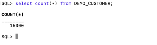
select count(*) from HR_INDEX;
   COUNT(*)
___________
        107
We can view what data is indexed by viewing the virtual document.
select json_serialize(DBMS_SEARCH.GET_DOCUMENT('HR_INDEX',METADATA))
from HR_INDEX;

JSON_SERIALIZE(DBMS_SEARCH.GET_DOCUMENT('HR_INDEX',METADATA))
___________________________________________________________________________________________________________________________________________________________________________________________________________________________________________________________________________
{"HR":{"EMPLOYEES":{"PHONE_NUMBER":"515.123.4567","JOB_ID":"AD_PRES","SALARY":24000,"COMMISSION_PCT":null,"FIRST_NAME":"Steven","EMPLOYEE_ID":100,"EMAIL":"SKING","LAST_NAME":"King","MANAGER_ID":null,"DEPARTMENT_ID":90,"HIRE_DATE":"2003-06-17T00:00:00"}}}
{"HR":{"EMPLOYEES":{"PHONE_NUMBER":"515.123.4568","JOB_ID":"AD_VP","SALARY":17000,"COMMISSION_PCT":null,"FIRST_NAME":"Neena","EMPLOYEE_ID":101,"EMAIL":"NKOCHHAR","LAST_NAME":"Kochhar","MANAGER_ID":100,"DEPARTMENT_ID":90,"HIRE_DATE":"2005-09-21T00:00:00"}}}
{"HR":{"EMPLOYEES":{"PHONE_NUMBER":"515.123.4569","JOB_ID":"AD_VP","SALARY":17000,"COMMISSION_PCT":null,"FIRST_NAME":"Lex","EMPLOYEE_ID":102,"EMAIL":"LDEHAAN","LAST_NAME":"De Haan","MANAGER_ID":100,"DEPARTMENT_ID":90,"HIRE_DATE":"2001-01-13T00:00:00"}}}
{"HR":{"EMPLOYEES":{"PHONE_NUMBER":"590.423.4567","JOB_ID":"IT_PROG","SALARY":9000,"COMMISSION_PCT":null,"FIRST_NAME":"Alexander","EMPLOYEE_ID":103,"EMAIL":"AHUNOLD","LAST_NAME":"Hunold","MANAGER_ID":102,"DEPARTMENT_ID":60,"HIRE_DATE":"2006-01-03T00:00:00"}}}
{"HR":{"EMPLOYEES":{"PHONE_NUMBER":"590.423.4568","JOB_ID":"IT_PROG","SALARY":6000,"COMMISSION_PCT":null,"FIRST_NAME":"Bruce","EMPLOYEE_ID":104,"EMAIL":"BERNST","LAST_NAME":"Ernst","MANAGER_ID":103,"DEPARTMENT_ID":60,"HIRE_DATE":"2007-05-21T00:00:00"}}}
We can search the metadata for certain data using the CONTAINS or JSON_TEXTCONTAINS functions.
select json_serialize(metadata)
from DEMO_IDX
where contains(data, 'winston')>0;
select json_serialize(metadata)
from DEMO_IDX
where json_textcontains(data, '$.HR.EMPLOYEES.FIRST_NAME', 'Winston');When the index is no longer required it can be dropped by running the following. Don’t run a DROP INDEX command as that removes some objects and leaves others behind! (leaves a bit of mess) and you won’t be able to recreate the index, unless you give it a different name.
exec dbms_search.drop_index('SH_INDEX');Number of rows in each Table – Various Databases
A possible common task developers perform is to find out how many records exists in every table in a schema. In the examples below I’ll show examples for the current schema of the developer, but these can be expanded easily to include tables in other schemas or for all schemas across a database.
These example include the different ways of determining this information across the main databases including Oracle, MySQL, Postgres, SQL Server and Snowflake.
A little warning before using these queries. They may or may not give the true accurate number of records in the tables. These examples illustrate extracting the number of records from the data dictionaries of the databases. This is dependent on background processes being run to gather this information. These background processes run from time to time, anything from a few minutes to many tens of minutes. So, these results are good indication of the number of records in each table.
Oracle
SELECT table_name, num_rows
FROM user_tables
ORDER BY num_rows DESC;
or
SELECT table_name,
       to_number(
          extractvalue(xmltype(
             dbms_xmlgen.getxml('select count(*) c from '||table_name))
                ,'/ROWSET/ROW/C')) tab_count
FROM   user_tables
ORDER BY tab_count desc;
Using PL/SQL we can do something like the following.
DECLARE
   val NUMBER;
BEGIN
   FOR i IN (SELECT table_name FROM user_tables ORDER BY table_name desc) LOOP
      EXECUTE IMMEDIATE 'SELECT count(*) FROM '|| i.table_name INTO val;
      DBMS_OUTPUT.PUT_LINE(i.table_name||' -> '|| val );
   END LOOP;
END;
MySQL
SELECT table_name, table_rows
FROM INFORMATION_SCHEMA.TABLES
WHERE table_type = 'BASE TABLE'
AND  TABLE_SCHEMA = current_user();
Using Common Table Expressions (CTE), using WITH clause
WITH table_list AS (
SELECT
    table_name
  FROM information_schema.tables
  WHERE table_schema = current_user()
  AND
        table_type = 'BASE TABLE'
)
SELECT CONCAT(
            GROUP_CONCAT(CONCAT("SELECT '",table_name,"' table_name,COUNT(*) rows FROM ",table_name) SEPARATOR " UNION "),
            ' ORDER BY table_name'
        )
INTO @sql
FROM table_list;
Postgres
select relname as table_name, n_live_tup as num_rows from pg_stat_user_tables;
An alternative is
select n.nspname as table_schema,
       c.relname as table_name,
       c.reltuples as rows
from pg_class c
join pg_namespace n on n.oid = c.relnamespace
where c.relkind = 'r'
      and n.nspname = current_user
order by c.reltuples desc;
SQL Server
SELECT tab.name,
       sum(par.rows)
FROM   sys.tables tab INNER JOIN sys.partitions par
          ON tab.object_id = par.object_id
WHERE  schema_name(tab.schema_id) = current_user
Snowflake
SELECT t.table_schema, t.table_name, t.row_count
FROM   information_schema.tables t
WHERE  t.table_type = 'BASE TABLE'
AND    t.table_schema = current_user
order by t.row_count desc;
The examples give above are some of the ways to obtain this information. As with most things, there can be multiple ways of doing it, and most people will have their preferred one which is based on their background and preferences.
As you can see from the code given above they are all very similar, with similar syntax, etc. The only thing different is the name of the data dictionary table/view containing the information needed. Yes, knowing what data dictionary views to query can be a little challenging as you switch between databases.
Postgres on Docker
Prostgres is one of the most popular databases out there, being used in Universities, open source projects and also widely used in the corporate marketplace. I’ve written a previous post on running Oracle Database on Docker. This post is similar, as it will show you the few simple steps to have a persistent Postgres Database running on Docker.
The first step is go to Docker Hub and locate the page for Postgres. You should see something like the following. Click through to the Postgres page.

There are lots and lots of possible Postgres images to download and use. The simplest option is to download the latest image using the following command in a command/terminal window. Make sure Docker is running on your machine before running this command.
docker pull postgresAlthough, if you needed to install a previous release, you can do that.

After the docker image has been downloaded, you can now import into Docker and create a container.
docker run --name postgres -p 5432:5432 -e POSTGRES_USER=postgres -e POSTGRES_PASSWORD=pgPassword -e POSTGRES_DB=postgres -d postgresImportant: I’m using Docker on a Mac. If you are using Windows, the format of the parameter list is slightly different. For example, remove the = symbol after POSTGRES_DB
If you now check with Docker you’ll see Postgres is now running on post 5432.

Next you will need pgAdmin to connect to the Postgres Database and start working with it. You can download and install it, or run another Docker container with pgAdmin running in it.
First, let’s have a look at installing pgAdmin. Download the image and run, accepting the initial requirements. Just let it run and finish installing.


When pgAdmin starts it looks for you to enter a password. This can be anything really, but one that you want to remember. For example, I set mine to pgPassword.
Then create (or Register) a connection to your Postgres Database. Enter the details you used when creating the docker image including username=postgres, password=pgPassword and IP address=0.0.0.0.
The IP address on your machine might be a little different, and to check what it is, run the following
docker ps -a


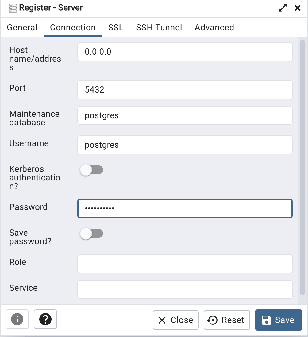
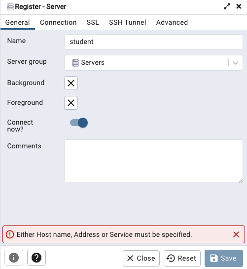
When your (above) connection works, the next step is to create another schema/user in the database. The reason we need to do this is because the user we connected to above (postgres) is an admin user. This user/schema should never be used for database development work.
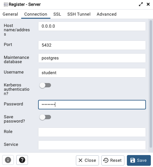
Let’s setup a user we can use for our development work called ‘student’. To do this, right click on the ‘postgres’ user connection and open the query tool.
Then run the following.

After these two commands have been run successfully we can now create a connection to the postgres database, open the query tool and you’re now all set to write some SQL.

Oracle Database In-Memory – simple example
In a previous post, I showed how to enable and increase the memory allocation for use by Oracle In-Memory. That example was based on using the Pre-built VM supplied by Oracle.
To use In-Memory on your objects, you have a few options.
Enabling the In-Memory attribute on the EXAMPLE tablespace by specifying the INMEMORY attribute
SQL> ALTER TABLESPACE example INMEMORY;Enabling the In-Memory attribute on the sales table but excluding the “prod_id” column
SQL> ALTER TABLE sales INMEMORY NO INMEMORY(prod_id);Disabling the In-Memory attribute on one partition of the sales table by specifying the NO INMEMORY clause
SQL> ALTER TABLE sales MODIFY PARTITION SALES_Q1_1998 NO INMEMORY;Enabling the In-Memory attribute on the customers table with a priority level of critical
SQL> ALTER TABLE customers INMEMORY PRIORITY CRITICAL;You can also specify the priority level, which helps to prioritise the order the objects are loaded into memory.

A simple example to illustrate the effect of using In-Memory versus not.
Create a table with, say, 11K records. It doesn’t really matter what columns and data are.
Now select all the records and display the explain plan
select count(*) from test_inmemory;
Now, move the table to In-Memory and rerun your query.
alter table test_inmemory inmemory PRIORITY critical;
select count(*) from test_inmemory;  -- again
There you go!
We can check to see what object are In-Memory by
SELECT table_name, inmemory, inmemory_priority, inmemory_distribute,
       inmemory_compression, inmemory_duplicate
FROM user_tables
WHERE inmemory = 'ENABLED’
ORDER BY table_name;
To remove the object from In-Memory
SQL > alter table test_inmemory no inmemory; -- remove the table from in-memory
This is just a simple test and lots of other things can be done to improve performance
But, you do need to be careful about using In-Memory. It does have some limitations and scenarios where it doesn’t work so well. So care is needed
Valintine’s Day SQL
Well today is February 14th and is know as (St.) Valintine’s Day. Here is a piece of SQL I just put together to mark today. Enjoy and Happy St. Valintine’s Day.
WITH heart_top(lev, love) AS (
   SELECT 1 lev, RPAD(' ', 7, ' ') || '**          **' love
   FROM dual
   UNION ALL
   SELECT heart_top.lev+1,
          RPAD(' ', 6-heart_top.lev*2, ' ') ||
          RPAD('*', (heart_top.lev*4)+2, '*') ||
          RPAD(' ', 11-heart_top.lev*3, ' ') ||
          RPAD('*', (heart_top.lev*4)+2, '*')  love
   FROM heart_top
   WHERE heart_top.lev < 4
),
   heart_bottom(lev, love) AS (
     SELECT 1 lev, '******************************' love
     FROM dual
     UNION ALL
     SELECT heart_bottom.lev+1,
          RPAD(' ', heart_bottom.lev*2, ' ') ||
          RPAD('*', 15-heart_bottom.lev*2, '*') ||
          RPAD('*', 15-heart_bottom.lev*2, '*')  love
     FROM heart_bottom
     WHERE heart_bottom.lev < 8
)
SELECT love FROM heart_top
union all
SELECT love FROM heart_bottom;
Which gives us the following.
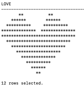
Bid you know : St. Valentine, the patron saint of love, was executed in Rome and buried there in the 3rd century. In 1835, an Irish priest was granted permission to exhume his remains, and now his skeleton lies in Whitefriar Church in Dublin city center.


You must be logged in to post a comment.