
Autonomous
oracledb Python Library – Connect to DB & a few other changes
Oracle have released a new Python library for connecting to Oracle Databases on-premises and on the Cloud. It’s called (very imaginatively, yet very clearly) oracledb. This new Python library replaces the previous library called cx_Oracle. Just consider cx_oracle as obsolete, and use oracledb going forward, as all development work on new features and enhancements will be done to oracledb.
cx_oracle has been around a long time, and it’s about time we have a new and enhanced library that is more flexible and will suit many different deployment scenarios. The previous library (cx_Oracle) was great, but it did require additional software installation with Oracle Client, and some OS environment settings, which at times took a bit of debugging. This makes it difficult/challenging to deploy in different environments, for example IOTs, CI/CD, containers, etc. Deployment environments have changed and the new oracledb library makes it simpler.
To check out the following links for a full list of new features and other details.
Home page: oracle.github.io/python-oracledb
Installation instructions: python-oracledb.readthedocs.io/en/latest/installation.html
Documentation: python-oracledb.readthedocs.io
One of the main differences between the two libraries is how you connect to the Database. With oracledb you need to use named the parameters, and the new library uses a thin connection. If you need the thick connection you can switch to that easily enough.
The following examples will illustrate how to connect to Oracle Database (local and cloud ADW/ATP) and how these are different to using the cx_Oracle library (which needed Oracle Client software installed). Remember the new oracledb library does not need Oracle Client.
To get started, install oracledb.
pip3 install oracledbLocal Database (running in Docker)
To test connection to a local Database I’m using a Docker image of 21c (hence localhost in this example, replace with IP address for your database). Using the previous library (cx_Oracle) you could concatenate the connection details to form a string and pass that to the connection. With oracledb, you need to use named parameters and specify each part of the connection separately.
This example illustrates this simple connection and prints out some useful information about the connection, do we have a healthy connection, are we using thing database connection and what version is the connection library.
p_username = "..."
p_password = "..."
p_dns = "localhost/XEPDB1"
p_port = "1521"

con = oracledb.connect(user=p_username, password=p_password, dsn=p_dns, port=p_port)

print(con.is_healthy())
print(con.thin)
print(con.version)
---

True
True
21.3.0.0.0
Having created the connection we can now query the Database and close the connection.
cur = con.cursor()
cur.execute('select table_name from user_tables')

for row in cur:
      print(row)

---
('WHISKIES_DATASET',)
('HOLIDAY',)
('STAGE',)
('DIRECTIONS',)
---

cur.close()
con.close()
The code I’ve given above is simple and straight forward. And if you are converting from cx_Oracle, you will probably have minimal changes as you probably had your parameter keywords defined in your code. If not, some simple editing is needed.
To simplify the above code even more, the following does all the same steps without the explicit open and close statements, as these are implicit in this example.
import oracledb

con = oracledb.connect(user=p_username, password=p_password, dsn=p_dns, port=p_port)
with con.cursor() as cursor:
  for row in cursor.execute('select table_name from user_tables'):
      print(row)
(Basic) Oracle Cloud – Autonomous Database, ATP/ADW
Everyone is using the Cloud, Right? If you believe the marketing they are, but in reality most will be working in some hybrid world using a mixture of on-premises and cloud storage. The example given in the previous section illustrated connecting to a local/on-premises database. Let’s now look at connecting to a database on Oracle Cloud (Autonomous Database, ATP/ADW).
With the oracledb library things have been simplified a little. In this section I’ll illustrate a simple connection to a ATP/ADW using a thin connection.
What you need is the location of the directory containing the unzipped wallet file. No Oracle client is needed. If you haven’t downloaded a Wallet file in a while, you should go download a new version of it. The Wallet will contain a pem file which is needed to securely connect to the DB. You’ll also need the password for the Wallet, so talk nicely with your DBA. When setting up the connection you need to provide the directory for the tnsnames.ora file and the ewallet.pem file. If you have downloaded and unzipped the Wallet, these will be in the same directory
import oracledb

p_username = "..."
p_password = "..."

p_walletpass = '...'

#This time we specify the location of the wallet
con = oracledb.connect(user=p_username, password=p_password, dsn="student_high",
                       config_dir="/Users/brendan.tierney/Dropbox/5-Database-Wallets/Wallet_student-Full",
                       wallet_location="/Users/brendan.tierney/Dropbox/5-Database-Wallets/Wallet_student-Full",
                       wallet_password=p_walletpass)

print(con)
con.close()
This method allows you to easily connect to any Oracle Cloud Database.
(Thick Connection) Oracle Cloud – Autonomous Database, ATP/ADW
If you have Oracle Client already installed and set up, and you want to use a thick connection, you will need to initialize the function init_oracle_client.
import oracledb

p_username = "..."
p_password = "..."

#point to directory containing tnsnames.ora
oracledb.init_oracle_client(config_dir="/Applications/instantclient_19_8/network/admin")

con = oracledb.connect(user=p_username, password=p_password, dsn="student_high")

print(con)

con.close()
Warning: Some care is needed with using init_oracle_client. If you use it once in your Python code or App then all connections will use it. You might need to do a code review to look at when this is needed and if not remove all occurrences of it from your Python code.
(Additional Security) Oracle Cloud – Autonomous Database, ATP/ADW
There are a few other additional ways of connecting to a database, but one of my favorite ways to connect involves some additional security, particularly when working with IOT devices, or in scenarios that additional security is needed. Two of these involve using One-way TLS and Mututal TLS connections. The following gives an example of setting up One-Way TLS. This involves setting up the Database to only received data and connections from one particular device via an IP address. This requires you to know the IP address of the device you are using and running the code to connect to the ATP/ADW Database.
To set this up, go to the ATP/ADW details in Oracle Cloud, edit the Access Control List, add the IP address of the client device, disable mutual TLS and download the DB Connection. The following code gives and example of setting up a connection
import oracledb

p_username = "..."
p_password = "..."

adw_dsn = '''(description= (retry_count=20)(retry_delay=3)(address=(protocol=tcps)(port=1522)
             (host=adb.us-ashburn-1.oraclecloud.com))(connect_data=(service_name=a8rk428ojzuffy_student_high.adb.oraclecloud.com))
             (security=(ssl_server_cert_dn="CN=adwc.uscom-east-1.oraclecloud.com,OU=Oracle BMCS US,O=Oracle Corporation,L=Redwood City,ST=California,C=US")))'''

con4 = oracledb.connect(user=p_username, password=p_password, dsn=adw_dsn)
This sets up a secure connection between the client device and the Database.
From my initial testing of existing code/applications (although no formal test cases) it does appear the new oracledb library is processing the queries and data quicker than cx_Oracle. This is good and hopefully we will see more improvements with speed in later releases.
Also don’t forget the impact of changing the buffer size for your database connection. This can have a dramatic effect on speeding up your database interactions. Check out this post which illustrates this.
OML4Py – AutoML – Step-by-Step Approach
Automated Machine Learning (AutoML) is or was a bit of a hot topic over the past couple of years. With various analysis companies like Gartner and others pushing for the need for AutoML, lots and lots of vendors have been creating different types of offerings to support this.
I’ve written some blog posts about AutoML already, from describing what it is and the different types, to showing how to do a black box approach using Oracle OML4Py, and also for using Oracle Machine Learning (OML) AutoML UI. Go check out those posts. In this post I will look at the more detailed step-by-step approach to AutoML using OML4Py. The same data set and cloud account/setup will be used. This will make it easier for you to compare the steps, the results and the AutoML experience across the different OML offerings.
Check out my previous post where I give details of the data set and some data preparation. I won’t repeat those here, but will move onto performing the step-by-step AutoML using OML4Py. The following diagram, from Oracle, outlines the steps involved

A little reminder/warning before you use AutoML in OML4Py. It only works for Classification (binary and multi-class) and Regression problems. The following code example illustrates a binary class problem, but in general there is no difference between the each type of Classification and Regression, except for the evaluation metrics, which I will list below.
Step 1 – Prepare the Data Set & Setup
See my previous blog post where I prepare the data set. I’m not going to repeat those steps here to save a little bit of space.
Also have a look at what libraries to load/import.
Step 2 – Automatic Algorithm Selection
The first step to configure and complete is select the “best model” from a selection of available Algorithms. Not all of the in-database algorithms are available to use in AutoML, which is a pity as there are some algorithms that can produce really accurate model. Hopefully with time these will be added.
The function to use is called AlgorithmSelection. This consists of two parts. The first is to define the parameters and the second part is to run it. This function accepts three parameters:
- mining function : ‘classification’ or ‘regression. Classification can be for binary and multi-class.
- score metric : the evaluation metric to evaluate the model performance. The following list gives the evaluation metric for each mining function
binary classification – accuracy (default), f1, precision, recall, roc_auc, f1_micro, f1_macro, f1_weighted, recall_micro, recall_macro, recall_weighted, precision_micro, precision_macro, precision_weighted
multiclass classification – accuracy (default), f1_micro, f1_macro, f1_weighted, recall_micro, recall_macro, recall_weighted, precision_micro, precision_macro, precision_weighted
regression – r2 (default), neg_mean_squared_error, neg_mean_absolute_error, neg_mean_squared_log_error, neg_median_absolute_error
- parallel : degree of parallelism to use. Default it system determined.
The second step uses this configuration and runs the code to find the “best models”. This takes the training data set (in typical Python format), and can also have a number of additional parameters. See my previous blog post for a full list of these, but ignore adaptive sampling. To keep life simple, you only really need to use ‘k’ and ‘cv’. ‘k’ specifies the number of models to include in the return list, default is 3. ‘cv’ tells how many levels of cross validation to perform. To keep things consistent across these blog posts and make comparison easier, I’m going to set ‘cv=5’
as_bank = automl.AlgorithmSelection(mining_function='classification',
                                    score_metric='accuracy', parallel=4)
oml_bank_ms = as_bank.select(oml_bank_X, oml_bank_y, cv=5)
To display the results and select out the best algorithm:
print("Ranked algorithms with Evaluation score:\n", oml_bank_ms)
selected_oml_bank_ms = next(iter(dict(oml_bank_ms).keys()))
print("Best algorithm =", selected_oml_bank_ms)

Ranked algorithms with Evaluation score:
 [('glm', 0.8668130990415336), ('glm_ridge', 0.8668130990415336), ('nb', 0.8634185303514377)]
Best algorithm = glm
This last bit of code is import, where the “best” algorithm is extracted from the list. This will be used in the next step.
“It Depends” is a phrase we hear/use a lot in IT, and the same applies to using AutoML. The model returned above does not mean it is the “best model”. It Depends on the parameters used, primarily the Evaluation Metric, but also the number set for CV (cross validation). Here are some examples of changing these and their results. As you can see we get a slightly different set of results or “best model” for each. My advice is to set ‘k’ large (eg current maximum values is 8), as this will ensure all algorithms are evaluated and not just a subset of them (potential hard coded ordered list of algorithms)
oml_bank_ms5 = as_bank.select(oml_bank_X, oml_bank_y, k=5)
oml_bank_ms5

[('glm', 0.8668130990415336), ('glm_ridge', 0.8668130990415336), ('nb', 0.8634185303514377), ('rf', 0.862020766773163), ('svm_linear', 0.8552316293929713)]
oml_bank_ms10 = as_bank.select(oml_bank_X, oml_bank_y, k=10)
oml_bank_ms10

[('glm', 0.8668130990415336), ('glm_ridge', 0.8668130990415336), ('nb', 0.8634185303514377), ('rf', 0.862020766773163), ('svm_linear', 0.8552316293929713), ('nn', 0.8496405750798722), ('svm_gaussian', 0.8454472843450479), ('dt', 0.8386581469648562)]
Here are some examples when the Score Metric is changed, and the impact it can have.
as_bank2 = automl.AlgorithmSelection(mining_function='classification',
                                     score_metric='f1', parallel=4)

oml_bank_ms2 = as_bank2.select(oml_bank_X, oml_bank_y, k=10)
oml_bank_ms2

[('rf', 0.6163242642976126), ('glm', 0.6160046056419113), ('glm_ridge', 0.6160046056419113), ('svm_linear', 0.5996686913307566), ('nn', 0.5896457765667574), ('svm_gaussian', 0.5829741379310345), ('dt', 0.5747368421052631), ('nb', 0.5269709543568464)]
as_bank3 = automl.AlgorithmSelection(mining_function='classification',
                                     score_metric='f1', parallel=4)

oml_bank_ms3 = as_bank3.select(oml_bank_X, oml_bank_y, k=10, cv=2)
oml_bank_ms3

[('glm', 0.60365647055431), ('glm_ridge', 0.6034077555816686), ('rf', 0.5990036646816308), ('svm_linear', 0.588201766334537), ('svm_gaussian', 0.5845019676714007), ('nn', 0.5842357537014313), ('dt', 0.5686862482989511), ('nb', 0.4981168003466766)]
as_bank4 = automl.AlgorithmSelection(mining_function='classification',
                                     score_metric='f1', parallel=4)

oml_bank_ms4 = as_bank4.select(oml_bank_X, oml_bank_y, k=10, cv=5)
oml_bank_ms4

[('glm', 0.583504644833276), ('glm_ridge', 0.58343736244422), ('rf', 0.5815952044164737), ('svm_linear', 0.5668069231027809), ('nn', 0.5628153929281711), ('svm_gaussian', 0.5613976370223811), ('dt', 0.5602129668741175), ('nb', 0.49153999668083814)]
The problem we now have with AutoML, it is telling us different answers for “best model”. To most that might be confusing but for the more technical data scientist they will know why. In very very simple terms, you are doing different things with the data and because of this you can get a different answer.
It is because of these different possible answers answers for the “best model”, is the reason AutoML can really only be used as a guide (a pointer towards what might be the “best model”), and cannot be relied upon to give a “best model”. AutoML is still not suitable for the general data analyst despite what some companies are saying.
Lots more could be discussed here but let’s more onto the next step.
Step 3 – Automatic Feature Selection
In the previous steps we have identified a possible “best model”. Let’s pretend the “best model” is the “best model”. The next steps is to look at how this model can be refined and improved using a subset of the features/attributes/columns. FeatureSelection looks are examining the data when combined with the model to find the optimised set of features/attributes/columns, to improve the model performance i.e. make it more accurate or have a better outcome based on the evaluation or score metric. For simplicity I’m going to use the result from the first example produced in the previous step. In a similar way to Step 2, there are two parts to setup and run the Feature Selection (Reduction). Each part is setup in a similar way to Step 2, with the parameters for FeatureSelection being the same values as those used for AlgorithmSelection. For the ‘reduce’ function, pass in the name of the “best model” or “best algorithm” from Step 2. This was extracted to a variable called ‘selected_oml_bank_ms’. Most of the other parameters the ‘reduce’ function takes are similar to the ‘select’ function. Again keeping things consistent, pass in the training data set and set the number of cross validations to 5.
fs_oml_bank = automl.FeatureSelection(mining_function = 'classification',
                                      score_metric = 'accuracy', parallel=4)

oml_bank_fsR = fs_oml_bank.reduce(selected_oml_bank_ms, oml_bank_X, oml_bank_y, cv=5)
We can now look at the results from this listing the reduced set of features/columns and comparing the number of features/columns in the original data set to the reduced set.
#print(oml_bank_fsR)
oml_bank_fsR_l = oml_bank_X[:,oml_bank_fsR]

print("Selected columns:", oml_bank_fsR_l.columns)
print("Number of columns:")
"{} reduced to {}".format(len(oml_bank_X.columns), len(oml_bank_fsR_l.columns))


Selected columns: ['DURATION', 'PDAYS', 'EMP_VAR_RATE', 'CONS_PRICE_IDX', 'CONS_CONF_IDX', 'EURIBOR3M', 'NR_EMPLOYED']
Number of columns:
'20 reduced to 7'
In this example the data set gets reduced from having 20 features/columns in the original data set, down to having 7 features/columns.
Step 4 – Automatic Model Tuning
Up to now, we have identified the “best model” / “best algorithm” and the optimised reduced set of features to use. The final step is to take the details generated from the previous steps and use this to generate a Tuned Model. In a similar way to the previous steps, this involve two parts. The first sets up some parameters and the second runs the Model Tuning function called ‘tune’. Make sure to include the data frame containing the reduced set of features/attributes.
mt_oml_bank = automl.ModelTuning(mining_function='classification', score_metric='accuracy', parallel=4)

oml_bank_mt = mt_oml_bank.tune(selected_oml_bank_ms, oml_bank_fsR_l, oml_bank_y, cv=5)

print(oml_bank_mt)
The output is very long and contains the name of the Algorithm, the hyperparameters used for the final model, the features used, and (at the end) lists the various combinations of hyperparameters used and the evaluation metric score for each combination. Partial output shown below.
mt_oml_bank = automl.ModelTuning(mining_function='classification', score_metric='accuracy', parallel=4)

oml_bank_mt = mt_oml_bank.tune(selected_oml_bank_ms, oml_bank_fsR_l, oml_bank_y, cv=5)
print(oml_bank_mt)

{'best_model':
Algorithm Name: Generalized Linear Model

Mining Function: CLASSIFICATION

Target: TARGET_Y

Settings:
setting name setting value
0 ALGO_NAME ALGO_GENERALIZED_LINEAR_MODEL
1 CLAS_WEIGHTS_BALANCED OFF
...
...
, 'all_evals': [(0.8544108809341562, {'CLAS_WEIGHTS_BALANCED': 'OFF', 'GLMS_NUM_ITERATIONS': 30, 'GLMS_SOLVER': 'GLMS_SOLVER_CHOL'}), (0.8544108809341562, {'CLAS_WEIGHTS_BALANCED': 'ON', 'GLMS_NUM_ITERATIONS': 30, 'GLMS_SOLVER': 'GLMS_SOLVER_CHOL'}), (0.8544108809341562, {'CLAS_WEIGHTS_BALANCED': 'OFF', 'GLMS_NUM_ITERATIONS': 31, 'GLMS_SOLVER': 'GLMS_SOLVER_CHOL'}), (0.8544108809341562, {'CLAS_WEIGHTS_BALANCED': 'OFF', 'GLMS_NUM_ITERATIONS': 173, 'GLMS_SOLVER': 'GLMS_SOLVER_CHOL'}), (0.8544108809341562, {'CLAS_WEIGHTS_BALANCED': 'OFF', 'GLMS_NUM_ITERATIONS': 174, 'GLMS_SOLVER': 'GLMS_SOLVER_CHOL'}), (0.8544108809341562, {'CLAS_WEIGHTS_BALANCED': 'OFF', 'GLMS_NUM_ITERATIONS': 337, 'GLMS_SOLVER': 'GLMS_SOLVER_CHOL'}), (0.8544108809341562, {'CLAS_WEIGHTS_BALANCED': 'OFF', 'GLMS_NUM_ITERATIONS': 338, 'GLMS_SOLVER': 'GLMS_SOLVER_CHOL'}), (0.8544108809341562, {'CLAS_WEIGHTS_BALANCED': 'ON', 'GLMS_NUM_ITERATIONS': 10, 'GLMS_SOLVER': 'GLMS_SOLVER_CHOL'}), (0.8544108809341562, {'CLAS_WEIGHTS_BALANCED': 'ON', 'GLMS_NUM_ITERATIONS': 173, 'GLMS_SOLVER': 'GLMS_SOLVER_CHOL'}), (0.8544108809341562, {'CLAS_WEIGHTS_BALANCED': 'ON', 'GLMS_NUM_ITERATIONS': 174, 'GLMS_SOLVER': 'GLMS_SOLVER_CHOL'}), (0.8544108809341562, {'CLAS_WEIGHTS_BALANCED': 'ON', 'GLMS_NUM_ITERATIONS': 337, 'GLMS_SOLVER': 'GLMS_SOLVER_CHOL'}), (0.8544108809341562, {'CLAS_WEIGHTS_BALANCED': 'ON', 'GLMS_NUM_ITERATIONS': 338, 'GLMS_SOLVER': 'GLMS_SOLVER_CHOL'}), (0.4211156437080018, {'CLAS_WEIGHTS_BALANCED': 'ON', 'GLMS_NUM_ITERATIONS': 10, 'GLMS_SOLVER': 'GLMS_SOLVER_SGD'}), (0.11374128955112069, {'CLAS_WEIGHTS_BALANCED': 'OFF', 'GLMS_NUM_ITERATIONS': 30, 'GLMS_SOLVER': 'GLMS_SOLVER_SGD'}), (0.11374128955112069, {'CLAS_WEIGHTS_BALANCED': 'ON', 'GLMS_NUM_ITERATIONS': 30, 'GLMS_SOLVER': 'GLMS_SOLVER_SGD'})]}
The list of parameter settings and the evaluation score is an ordered list in decending order, starting with the best model.
We can extract the different parts of this dictionary object by using the following:
#display the main model details
print(oml_bank_mt['best_model'])
Now extract the evaluation metric score and the parameter settings used for the best model, (position 0 of the dictionary)
score, params = oml_bank_mt['all_evals'][0]
And that’s it, job done with using OML4Py AutoML to generate an optimised model.
The example above is for a Classification problem. If you had a Regression problem all you need to do is replace ‘classification’ with ‘regression’, and change the score_metric parameter to ‘r2’, or one of the other Regression metric values (see above for list of these.
OML4Py – AutoML – An Example
OML4Py (Oracle Machine Learning for Python) is Oracle’s offering where you can use Python commands to process and analyse data in an Oracle Database without having to write any SQL. OML4Py, via it’s transparency layer, translates Python code into SQL, executes it in the Database and then presents the results back to you in your Python environment. The examples shown in this post used the OML Notebooks available with Autonomous Databases on Oracle Cloud.
[Warning: the functionality available with initial release of OML4Py is very limited and may not suit most Python developers. Hopefully this will be addressed in later releases]
One of the features of OML4Py is Automated Machine Leaning (AutoML). At some point in the near future Oracle will have a GUI interface for AutoML, which will save you from having to write any code, such as the example in this post. See my previous blog post about AutoML. It is a general discussion on AutoML and some things you need to be careful with. Also, be careful of the marketing around AutoML from all vendors. The reality doesn’t necessarily live up to marketing

OML4Py has a couple of approaches you can follow to Automatically generate a Machine Learning Model (see previous blog post). The first of these can be considered the Black Box approach for AutoML, and the example below illustrates an example of this. The more detailed version of AutoML will be covered in a later post.
[Info: I’m using Oracle Free Tier Database. At time of writing this post OML4Py is only available with Oracle Autonomous 19c]
But before look at these, the first step we need to do is setup the data set to use for AutoML. I’ll be using the popular Portuguese Bank data set. Each code snippets shown below are for a one cell in my OML Notebooks. The data set exists as a table in my schema called BANK_ADDITIONAL_FULL. The sync command creates a proxy object in the notebook session pointing to the table in the DB. No data is copied into the notebook.
%python
import oml
from oml import automl
import pandas as pd
%python
oml_bank = oml.sync(table = 'BANK_ADDITIONAL_FULL')
type(oml_bank)
Let’s explore the data. Remember the data lives in a table in the DB and only the results are displayed
%python
oml_bank.head()

%python
oml_bank.describe()

Now remove one attribute from data set and at the sample time setup the dataframes for input to the ML. This is highly correlated to the the target variable.
%python
oml_bank_X, oml_bank_y = oml_bank.drop('TARGET_Y'), oml_bank['TARGET_Y']
Finally, we can now look at the first of the AutoML options, the black box option. This uses the AutoML ModelSelection function. Using this you can define the type of machine learning to perform (‘classification) and set some additional parameters. The parallel parameter will probably not have too much of an effect when using the Oracle Free Tier, but will certainly improved performance when using additional compute resources.
The example below is very simple and the setup of it is very simple. The ModelSelection function sets up the parameters for the AutoML to function. The ‘select’ function runs the AutoML based on those parameters along with some additional ones. These parameters and the additional ones available are explained below, after this first example.
%python
ms_bank = automl.ModelSelection(mining_function='classification', parallel=4)
ModelSelection can have the following parameters. The possible values for each are listed with the value in bold being the default value:
- mining_function : the type of ML to preform, only two option available for this, classification or regression
- score_metric: what metric to use for evaluating the models. Defaults for binary and multi classification balanced_accuracy is used and default for regression is neg_mean_squared_error. Other options for regression include r2, neg_mean_absolute_error and neg_median_absolute_error. For classification other options include, accuracy, f1, precision, recall, roc_auc, f1_micro, f1_macro, f1_weighted, recall_micro, recall_macro, recall_weighted, precision_micro, precision_macro, precision_weighted
- parallel: degree of parallelism to use, None or a number.
Having defined ModelSelection settings, we can move onto using it to preform (black box) AutoML, using the ‘select’ function. Oracle doesn’t tell us what it does inside this black box except that it uses ML and meta-learning techniques to work out which algorithms to use, what subsets of the original data set to use to give use a optimal outcome. It’s there secret recipe!
The ‘select’ function elevates all the available algorithms, creating models for each or a subset of them based on the meta-learning, and returns the “best” one. The function returns just one model, which is the “best”. The value set for ‘k’ tells the function how many of the “best” or top models created, how many of these to tune before returning the “best” one.
Now, let’s run an example of the ‘select’ function and what parameters is can have
- X: input data set consisting of the columns to use for Training.
- y: the column containing the Target variable.
- case_id: columns name of case_id, default is None. If supplied can be used for data sampling
- k: the number of (best) models to tune. Default is 3, but can be set to any number between one and eight, as setting it higher than that has no effect as there aren’t any more than that number of algorithms in the database!
- solver: allowed values are fast (default) and exhaustive. fast uses internal ML and meta-learning thereby reducing the search space. exhaustive will be slower as it will evaluate all algorithms and options for creating a model.
- cv: cross validation. Default is auto, but can be set to a number or set to None uses inputs defined in X_valid and y_valid defined below. auto will determine the number based on size of input data set, and when a number is provided will perform that number cross validation.
- adaptive_sampling: use adaptive sampling to reduce data set size to speed up runtime of ‘select’ function. Default is True, otherwise use False.
- X_valid: validation data set, default is None.
- y_valid: validation target column, default is None.
- time_budget: defines a time constraint on how how long, in seconds, to spend working out the solution. Default is None, or number for number of seconds. Useful for large data sets or for when you need a quicker results, and can be increased based on experimentation.
Here is a basic example of using the ‘select’ function, using the data frames created above as input, ‘k’ is set to five telling the function to tune the top five models created based on doing five fold cross-validation ‘cv’.
best_model = ms_bank.select(oml_bank_X, oml_bank_y, k=5, cv=5)
best_model
This returns the following model information. We are told the algorithm used (RandomForest), the tuned algorithm settings, and what attributes from the input data frame are used in the tuned model.
(
Algorithm Name: Random Forest

Mining Function: CLASSIFICATION

Target: TARGET_Y

Settings:
setting name setting value
0 ALGO_NAME ALGO_RANDOM_FOREST
1 CLAS_MAX_SUP_BINS 32
2 CLAS_WEIGHTS_BALANCED OFF
3 ODMS_DETAILS ODMS_DISABLE
4 ODMS_MISSING_VALUE_TREATMENT ODMS_MISSING_VALUE_AUTO
5 ODMS_RANDOM_SEED 0
6 ODMS_SAMPLING ODMS_SAMPLING_DISABLE
7 PREP_AUTO ON
8 RFOR_MTRY 10
9 RFOR_NUM_TREES 20
10 RFOR_SAMPLING_RATIO 0.5
11 TREE_IMPURITY_METRIC TREE_IMPURITY_ENTROPY
12 TREE_TERM_MAX_DEPTH 16
13 TREE_TERM_MINPCT_NODE 0.05
14 TREE_TERM_MINPCT_SPLIT 0.1
15 TREE_TERM_MINREC_NODE 10
16 TREE_TERM_MINREC_SPLIT 20

Attributes:
AGE
CAMPAIGN
CONS_CONF_IDX
CONS_PRICE_IDX
CONTACT
DEFAULT_VALUE
DURATION
EDUCATION
EMP_VAR_RATE
EURIBOR3M
JOB
MARITAL
MONTH
NR_EMPLOYED
PDAYS
POUTCOME
PREVIOUS

Partition: NO

, 'rf')
[I’ve found the Oracle Documentation for (initial release of) OML4Py lacking with information. Hopefully the documentation will be updated]
I’ve mentioned before you need to exercise some caution with using AutoML due to various potential legal and moral issues. Can they be used as a quick way get an idea if ML will produce useful insights for your data. But the results from it should never be used for making business decisions and never deployed in production. Use it as a starting point, from which to build out an ML solutions with humans making the decisions on what to use and why to use them.
For a more detailed, step-by-step approach to AutoML check out this next post for more.
[Warning: Based on the functionality currently available in this early release of OML4Py, you will be limited in what you can do, not just with AutoML but with other features of OML4Py. Maybe check back at a later time when it has matured and has way more functionality, allowing you to do something useful with it!]
OML Notebooks Interpreter Bindings
When using Oracle Machine Learning notebooks, you can export and import these between different projects and different environments (from ADW to ATP).
But something to watch out for when you import a notebook into your ADW or ATP environment is to reset the Interpreter Bindings.
When you create a new OML Notebook and build it up, the various Interpreter Bindings are automatically set or turned on. But for Imported OML Notebooks they are not turned on.
I’m assuming this will be fixed at some future point.
If you import an OML Notebook and turn on the Interpreter Bindings you may find the code in your notebook cells running very slowly
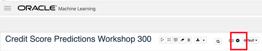
To turn on these binding, click on the options icon as indicated by the red box in the following image.
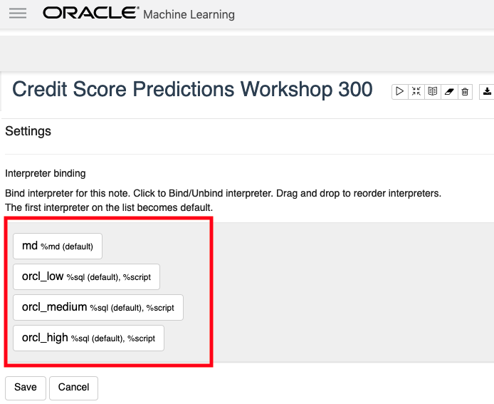
You will get something like the following being displayed. None of the bindings are highlighted.
To enable the Interpreter Bindings just click on each of these boxes. When you do this each one will be highlighted and will turn a blue color.
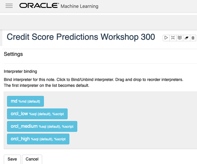
All done! You can now run your OML Notebooks without any problems or delays.
Oracle Machine Learning notebooks
With the recent release of Oracle’s Autonomous Data Warehouse Cloud (ADWC), Oracle has given data scientists a new tool for data discovery and machine learning on the ADWC. Oracle Machine Learning is based on Apache Zeppelin and gives us a new machine learning tool for accessing the in-database machine learning algorithms and in-database statistical functions.
Oracle Machine Learning (OML) SQL notebooks provide easy access to Oracle’s parallelized, scalable in-database implementations of a library of Oracle Advanced Analytics’ machine learning algorithms (classification, regression, anomaly detection, clustering, associations, attribute importance, feature extraction, times series, etc.), SQL, PL/SQL and Oracle’s statistical and analytical SQL functions. Oracle Machine Learning SQL notebooks and Oracle Advanced Analytics’ library of machine learning SQL functions combined with PL/SQL allow companies to automate their discovery of new insights, generate predictions and add “AI” to data viz dashboards and enterprise applications.
The key features of Oracle Machine Learning include:
- Collaborative SQL notebook UI for data scientists
- Packaged with Oracle Autonomous Data Warehouse Cloud
- Easy access to shared notebooks, templates, permissions, scheduler, etc.
- Access to 30+ parallel, scalable in-database implementations of machine learning algorithms
- SQL and PL/SQL scripting language supported
- Enables and Supports Deployments of Enterprise Machine Learning Methodologies in ADWC
Here is a list of key resources for Oracle Machine Learning:
- Oracle Machine Learning Notebooks
- Video overview of Oracle Machine Learning
- Download sample Oracle Machine Learning notebooks
- Quick Start Tutorial for getting started with Oracle Machine Learning
- Documentation: Using Oracle Machine Learning


You must be logged in to post a comment.