
AutoML
AutoML using Pycaret
In this post we will have a look at using the AutoML feature in the Pycaret Python library. AutoML is a popular topic and allows Data Scientists and Machine Learning people to develop potentially optimized models based on their data. All requiring the minimum of input from the Data Scientist. As with all AutoML solutions, care is needed on the eventual use of these models. With various ML and AI Legal requirements around the World, it might not be possible to use the output from AutoML in production. But instead, gives the Data Scientists guidance on creating an optimized model, which can then be deployed in production. This facilitates requirements around model explainability, transparency, human oversight, fairness, risk mitigation and human in the loop.
Some useful links
Pycaret as all your typical Machine Learning algorithms and functions, including for classification, regression, clustering, anomaly detection, time series analysis, and so on.
To install Pycaret run the typical pip command
pip3 install pycaret
If you get any error messages when running any of the following example code, you might need to have a look at your certificates. Locate where Python is installed (for me on a Mac /Applications/Python 3.7) and you will find a command called ‘Install Certificates.command’. and run the following in the Python directory. This should fix what is causing the errors.
Pycaret comes with some datasets. Most of these are the typical introduction datasets you will find in other Python libraries and in various dataset repositories. For our example we are going to use the Customer Credit dataset. This contains data for a classification problem and the aim is to predict customers who are likely to default.
Let’s load the data and have a quick explore
#Don't forget to install Pycaret
#pip3 install pycaret

#Import dataset from Pycaret
from pycaret.datasets import get_data

#Credit defaulters dataset
df = get_data("credit")
The dataframe is displayed for the first five records
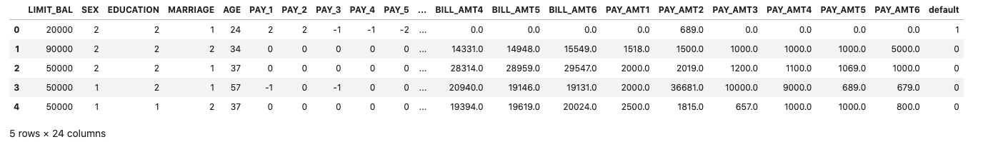
What’s the shape of the dataframe? The dataset/frame has 24,000 records and 24 columns.
#Check for the shape of the dataset
df.shape

(24000, 24)
The dataset has been formatted for a Classification problem with the column ‘default’ being the target or response variable. Let’s have a look at the distribution of records across each value in the ‘default’ column.
df['default'].value_counts()

0    18694
1     5306
And to get the percentage of these distributions,
df['default'].value_counts(normalize=True)*100

0    77.891667
1    22.108333
Before we can call the AutoML function, we need to create our Training and Test datasets.
#Initialize seed for random generators and reproducibility
seed = 42

#Create the train set using pandas sampling - seen data set
train = df.sample(frac=.8, random_state=seed)
train.reset_index(inplace=True, drop=True)
print(train.shape)
train['default'].value_counts()

(19200, 24)

0    14992
1     4208
Now the Test dataset.
#Using samples not available in train as future or unseen data set
test = df.drop(train.index)
test.reset_index(inplace=True, drop=True)
print(test.shape)
test['default'].value_counts()

(4800, 24)

0    3798
1    1002
Next we need to setup and configure the AutoML experiment.
#Let's Do some magic!
from pycaret.classification import *

#Setup function initializes the environment and creates the transformation pipeline
clf = setup(data=train, target="default", session_id=42)
When the above is run, it goes through a number of steps. The first looks at the dataset, the columns and determines the data types, displaying the following.

If everything is correct, press the enter key to confirm the datatypes, otherwise type ‘quit‘. If you press enter Pycaret will complete the setup of the experiments it will perform to identify a model. A subset of the 60 settings is shown below.

The next step runs the experiments to compare each of the models (AutoML), evaluates them and then prints out a league table of models with values for various model evaluation measures. 5.-Fold cross validation is used for each model. This league table is updated are each model is created and evaluated.
# Compares different models depending on their performance metrics. By default sorted by accuracy
best_model = compare_models(fold=5)
For this dataset, this process of comparing the models (AutoML) only takes a few seconds. The constant updating of the league tables is a nice touch. The following shows the final league table created for our AutoML.

The cells colored/highlighted in Yellow tells you which model scored based for that particular evaluation matrix. Here we can see Ridge Classifier scored best using Accuracy and Precision. While the Linear Discriminant Analysis model was best using F1 score, Kappa and MCC.
print(best_model)

RidgeClassifier(alpha=1.0, class_weight=None, copy_X=True, fit_intercept=True,
                max_iter=None, normalize=False, random_state=42, solver='auto',
                tol=0.001)
We can also print the ROC chart.
# Plots the AUC curve
import matplotlib.pyplot as plt

fig = plt.figure()
plt.figure(figsize = (14,10))
plot_model(best_model, plot="auc", scale=1)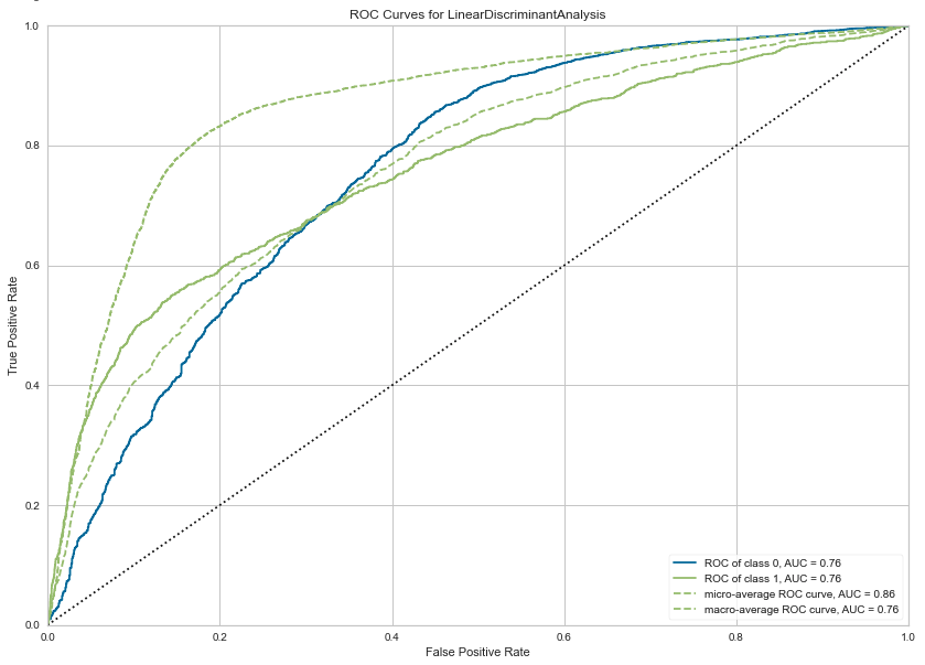
Also the confusion matrix.
plot_model(best_model, plot="confusion_matrix")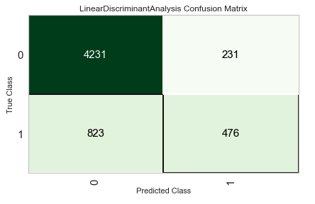
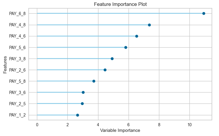
We can also see what the top features are that contribute to the model outcomes (the predictions). This is also referred to as feature importance.
plot_model(best_model, plot="feature")
We could take one of these particular models and tune it for a better fit, or we could select the ‘best’ model and tune it.
# Tune model function performs a grid search to identify the best parameters
tuned = tune_model(best_model)
We can now use the tuned model to label the Test dataset and compare the results.
# Predict on holdout set
predict_model(tuned, data=test)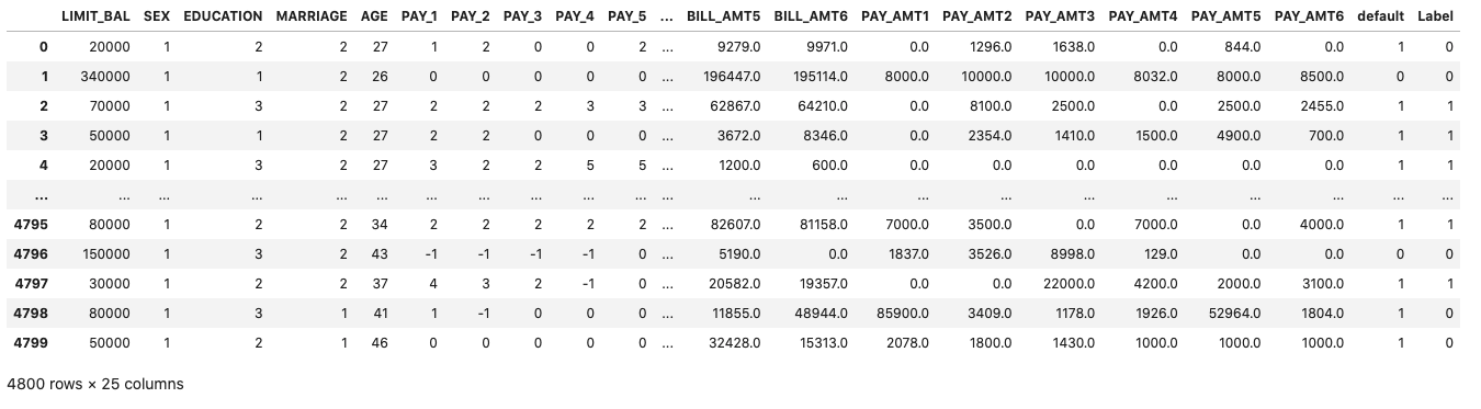
The final steps with all models is to save it for later use. Pycaret allows you to save the model in .pkl file format
# Model will be saved as .pkl and can be utilized for serving
save_model(tuned,'Tuned-Model-AutoML-Pycaret')
That’s it. All done.
AutoML – using TPOT
Another popular AutoML library is TPOT, which stands for Tree-Based Pipeline Optimization Tool. The goal of TPOT is to automate the building of ML pipelines by combining a flexible expression tree representation of pipelines with stochastic search algorithms such as genetic programming. TPOT makes use of the Python-based scikit-learn library
Install the TPOT library using
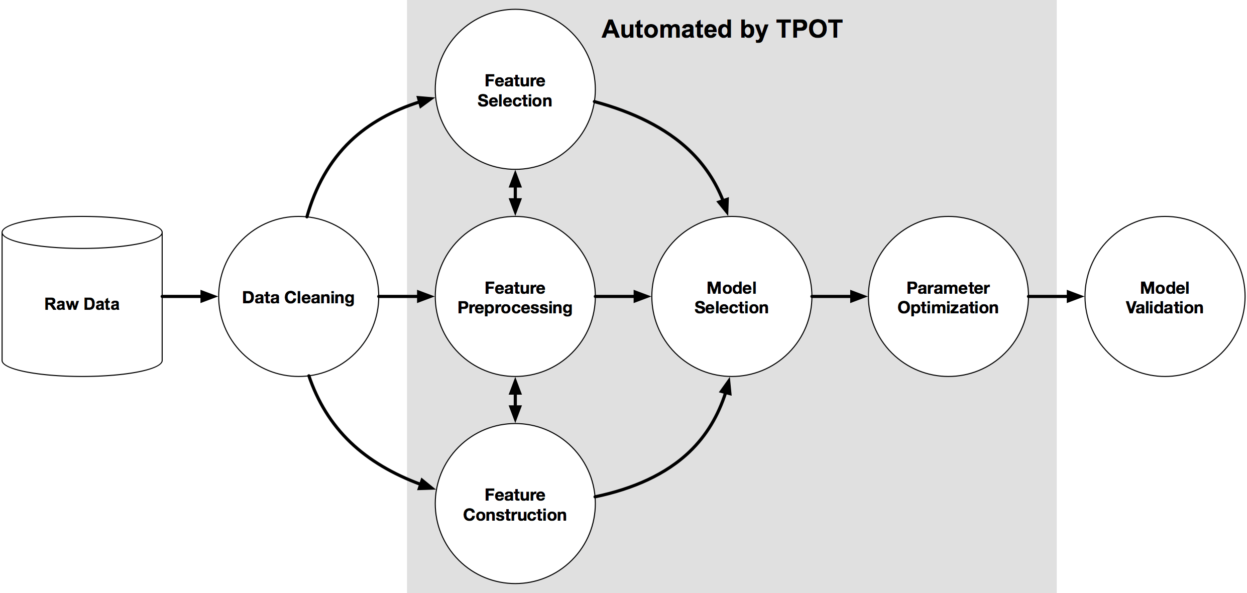
pip3 install tpotHere is an example tree-based pipeline from TPOT. Each circle corresponds to a machine learning operator, and the arrows indicate the direction of the data flow

Let’s build upon my previous blog post on AutomML, by using the same data set, with no modifications, and using the training (X_train, y_train) and test (X_test, y_test) data sets (dataframes), based on the Bank data sets. Check the previous post for the detailed steps on getting to this point.
In a similar way as the autosklean library example, I’m just going to demonstrate using TPOT for a classification problem using TPOTClassifier class. For regression problems, there is the corresponding TPOTRegressor class (not demonstrated in this post).
TPOTClassifier has the following main parameters (there are others):
- generations: Number of iterations to the run pipeline optimization process. The default is 100.
- population_size: Number of individuals to retain in the genetic programming population every generation. The default is 100.
- offspring_size: Number of offspring to produce in each genetic programming generation. The default is 100.
- mutation_rate: Mutation rate for the genetic programming algorithm in the range [0.0, 1.0]. This parameter tells the GP algorithm how many pipelines to apply random changes to every generation. Default is 0.9
- crossover_rate: Crossover rate for the genetic programming algorithm in the range [0.0, 1.0]. This parameter tells the genetic programming algorithm how many pipelines to “breed” every generation.
- scoring: Function used to evaluate the quality of a given pipeline for the classification problem like
accuracy,average_precision,roc_auc,recall, etc. The default isaccuracy. - cv: Cross-validation strategy used when evaluating pipelines. The default is 5.
- random_state: The seed of the pseudo-random number generator used in TPOT. Use this parameter to make sure that TPOT will give you the same results each time you run it against the same data set with that seed.
- verbosity: How much information TPOT communicates while it is running. Default is 0 (zero) TPOT will display nothing. 1=display minimal information, 2=display more information and progress bar, 3=print everything and progress bar.
- n_jobs: Number of processes to use. Default is 1. Use -1 to use all available cores.
Care is needed with some of these settings, for example generations should be set small to begin with, for example set to 5 initially. Also, population_size should also be kept small, for example 5 initially. These initial settings will evaluate 25 piplelines (5×5) configurations before finishing, and for some these settings may need to be adjusted smaller for initial work/investigations. Another parameter to adjust is the ‘verbosity’ setting. The default is 0 which means no details will be displayed. I like to set this to 3, as it gives more details of the outcomes from each pipeline. Adjust higher for more details or lower to fewer details. Another parameter to consider adjusting is ‘max_time_min’ and ‘max_eval_time_min’, but setting these too low can result in no or minimum results.
Load the library, setup the configuration and run. This is very simple to setup
from tpot import TPOTClassifier

#configure settings
tpot = TPOTClassifier(generations=5, population_size=5, verbosity=3, n_jobs=4, scoring='accuracy')

#run TPOT
tpot.fit(X_train, y_train)
As verbosity is set to 3 we get a lot of detail being displayed for each generation. The final output is shown below. What is missing from this is the progress bars which are displayed while TPOT is running
32 operators have been imported by TPOT.


Generation 1 - Current Pareto front scores:

-1	0.8963961891371728	RandomForestClassifier(input_matrix, RandomForestClassifier__bootstrap=True, RandomForestClassifier__criterion=gini, RandomForestClassifier__max_features=0.7000000000000001, RandomForestClassifier__min_samples_leaf=5, RandomForestClassifier__min_samples_split=7, RandomForestClassifier__n_estimators=100)

-2	0.8978183008194085	RandomForestClassifier(ZeroCount(input_matrix), RandomForestClassifier__bootstrap=True, RandomForestClassifier__criterion=gini, RandomForestClassifier__max_features=0.7000000000000001, RandomForestClassifier__min_samples_leaf=5, RandomForestClassifier__min_samples_split=7, RandomForestClassifier__n_estimators=100)
Pipeline encountered that has previously been evaluated during the optimization process. Using the score from the previous evaluation.

Generation 2 - Current Pareto front scores:

-1	0.8974020496851336	RandomForestClassifier(input_matrix, RandomForestClassifier__bootstrap=True, RandomForestClassifier__criterion=gini, RandomForestClassifier__max_features=0.7000000000000001, RandomForestClassifier__min_samples_leaf=8, RandomForestClassifier__min_samples_split=7, RandomForestClassifier__n_estimators=100)

-2	0.8978183008194085	RandomForestClassifier(ZeroCount(input_matrix), RandomForestClassifier__bootstrap=True, RandomForestClassifier__criterion=gini, RandomForestClassifier__max_features=0.7000000000000001, RandomForestClassifier__min_samples_leaf=5, RandomForestClassifier__min_samples_split=7, RandomForestClassifier__n_estimators=100)
_pre_test decorator: _random_mutation_operator: num_test=0 '(slice(None, None, None), 0)' is an invalid key.
Pipeline encountered that has previously been evaluated during the optimization process. Using the score from the previous evaluation.

Generation 3 - Current Pareto front scores:

-1	0.8974020496851336	RandomForestClassifier(input_matrix, RandomForestClassifier__bootstrap=True, RandomForestClassifier__criterion=gini, RandomForestClassifier__max_features=0.7000000000000001, RandomForestClassifier__min_samples_leaf=8, RandomForestClassifier__min_samples_split=7, RandomForestClassifier__n_estimators=100)

-2	0.8978183008194085	RandomForestClassifier(ZeroCount(input_matrix), RandomForestClassifier__bootstrap=True, RandomForestClassifier__criterion=gini, RandomForestClassifier__max_features=0.7000000000000001, RandomForestClassifier__min_samples_leaf=5, RandomForestClassifier__min_samples_split=7, RandomForestClassifier__n_estimators=100)
Skipped pipeline #21 due to time out. Continuing to the next pipeline.
Skipped pipeline #23 due to time out. Continuing to the next pipeline.

Generation 4 - Current Pareto front scores:

-1	0.8974020496851336	RandomForestClassifier(input_matrix, RandomForestClassifier__bootstrap=True, RandomForestClassifier__criterion=gini, RandomForestClassifier__max_features=0.7000000000000001, RandomForestClassifier__min_samples_leaf=8, RandomForestClassifier__min_samples_split=7, RandomForestClassifier__n_estimators=100)

-2	0.8978183008194085	RandomForestClassifier(ZeroCount(input_matrix), RandomForestClassifier__bootstrap=True, RandomForestClassifier__criterion=gini, RandomForestClassifier__max_features=0.7000000000000001, RandomForestClassifier__min_samples_leaf=5, RandomForestClassifier__min_samples_split=7, RandomForestClassifier__n_estimators=100)

Generation 5 - Current Pareto front scores:

-1	0.8983385200075953	RandomForestClassifier(input_matrix, RandomForestClassifier__bootstrap=True, RandomForestClassifier__criterion=gini, RandomForestClassifier__max_features=0.55, RandomForestClassifier__min_samples_leaf=8, RandomForestClassifier__min_samples_split=7, RandomForestClassifier__n_estimators=100)

TPOTClassifier(generations=5, n_jobs=4, population_size=5, scoring='accuracy',
               verbosity=3)
We can now display the ‘best’ model configuration discovered by TPOT.
tpot.fitted_pipeline_


Pipeline(steps=[('normalizer', Normalizer(norm='l1')),
                ('xgbclassifier',
                 XGBClassifier(base_score=0.5, booster='gbtree',
                               colsample_bylevel=1, colsample_bynode=1,
                               colsample_bytree=1, gamma=0, gpu_id=-1,
                               importance_type='gain',
                               interaction_constraints='', learning_rate=0.01,
                               max_delta_step=0, max_depth=8,
                               min_child_weight=7, missing=nan,
                               monotone_constraints='()', n_estimators=100,
                               n_jobs=1, num_parallel_tree=1, random_state=0,
                               reg_alpha=0, reg_lambda=1, scale_pos_weight=1,
                               subsample=0.8, tree_method='exact',
                               validate_parameters=1, verbosity=0))])
In this run of TPOT, on this data set, XGBoost algorithm gave the best results using the parameters and settings listed above. What is interesting, everytime I’ve run TPOT for the same data set, using the same configuration parameters, I get a slightly different outcome.
Next step is to evaluate the ‘best’ model on the holdout data set.
tpot.score(X_test, y_test)


0.9037792344420167
The results achieved are good and are better than some of the other models created by other AutoML libraries.
The final step we can perform is to export the model template. This creates a file containing the template code to create and use the model. This does require some modifications to specify the data set, and the pipeline of data modifications and transformations.
#export the model
tpot.export('.../tpot_Bank_pipeline.py')
The output file contains the following.
import numpy as np
import pandas as pd
from sklearn.model_selection import train_test_split
from sklearn.pipeline import make_pipeline
from sklearn.preprocessing import Normalizer
from xgboost import XGBClassifier

# NOTE: Make sure that the outcome column is labeled 'target' in the data file
tpot_data = pd.read_csv('PATH/TO/DATA/FILE', sep='COLUMN_SEPARATOR', dtype=np.float64)
features = tpot_data.drop('target', axis=1)

training_features, testing_features, training_target, testing_target = \
            train_test_split(features, tpot_data['target'], random_state=None)

# Average CV score on the training set was: 0.8986507248984001
exported_pipeline = make_pipeline(
    Normalizer(norm="l1"),
    XGBClassifier(learning_rate=0.01, max_depth=8, min_child_weight=7, n_estimators=100, n_jobs=1, subsample=0.8, verbosity=0)
)

exported_pipeline.fit(training_features, training_target)
results = exported_pipeline.predict(testing_features)
TPOT does have some issues and limitations. Well it is slow, and part of this is due to the nature of genetic algorithms, every time you run TPOT you may get different results, etc. Some of these issues can be addressed by adjusting some of the parameters, but even still, it doesn’t eliminate all of them. Running on GPU helps a little with timing of each run. TPOT doesn’t remove the need for data cleaning, feature engineering etc, but that is the case with most solutions.
AutoML – using autosklearn in Python
I’ve written some previous posts about AutoML and how to use AutoML with Oracle OML4Py (part 1 and part 2) and AutoML UI.
Building upon these, in this post I’ll demonstrate how to use autosklearn Python Package to do something similar, using the same data set I used in my previous posts.
To install the package run the typical pip command
pip3 install auto-sklearn
I did have some challegenges with installing this package, and this seems to be common, with different people having slightly different issues. These mainly revolved around having to install/update the swiff and pyrfr Python packages. Once done, then autosklearn package installed.
Let’s do a simple test
import autosklearn
print('autosklearn: %s' % autosklearn.__version__)

autosklearn: 0.12.5
Just like in my previous examples, I’m just going to use autosklearn to build a Classification model, as that is what the data set is designed for.
from sklearn.metrics import accuracy_score

# define search
model = autosklearn.classification.AutoSklearnClassifier()
# perform the search
model.fit(X_train, y_train)
The code above is a very basic configuration, and if this is the first time you are going to run this, then DON’T. There are a lot of parameter you can set, with one of them being ‘time_left_for_this_task’. The default value for this parameter is 360, which is one hour. Not a good idea! Set this to being much lower, say for an initial run of 3-5 minutes. This should be enough time for it to build many different models. I like to set the time for this using a multiplier of 60 (seconds). That way you don’t have to do any calculations! Two other parameters to consider setting/changing are
- n_jobs: this is the number of jobs to run in parallel. Default is -1, which uses all processors, or set to to a number, eg. 4
- metric: what evaluation metric to use for the models. For classification we have, accuracy, balanced_accuracy, f1, f1_marco, f1_micro, f1_samples, f1_weighted, roc_auc, precision, precision_macro, precision_micro, precision_samples, precision_weighted, average_percision, recall, recall_macro, recall_micro, recall_samples, recall_weighted and log_loss. For regression problems, r2, mean_squared_error, mean_absolute_error and median_absolute_error
Using these parameters let’s run a search.
# define search
model2 = autosklearn.classification.AutoSklearnClassifier(time_left_for_this_task=2*60,
      n_jobs=-1,
      metric=autosklearn.metrics.accuracy)

# perform the search
model2.fit(X_train, y_train)

Out[]: AutoSklearnClassifier(metric=accuracy, n_jobs=-1, per_run_time_limit=48,
                      time_left_for_this_task=120)
After about 2 minutes we explore the models.
print(model2.show_models())

[(0.520000, SimpleClassificationPipeline({'balancing:strategy': 'none', 'classifier:__choice__': 'random_forest', 'data_preprocessing:categorical_transformer:categorical_encoding:__choice__': 'one_hot_encoding', 'data_preprocessing:categorical_transformer:category_coalescence:__choice__': 'minority_coalescer', 'data_preprocessing:numerical_transformer:imputation:strategy': 'mean', 'data_preprocessing:numerical_transformer:rescaling:__choice__': 'standardize', 'feature_preprocessor:__choice__': 'no_preprocessing', 'classifier:random_forest:bootstrap': 'True', 'classifier:random_forest:criterion': 'gini', 'classifier:random_forest:max_depth': 'None', 'classifier:random_forest:max_features': 0.5, 'classifier:random_forest:max_leaf_nodes': 'None', 'classifier:random_forest:min_impurity_decrease': 0.0, 'classifier:random_forest:min_samples_leaf': 1, 'classifier:random_forest:min_samples_split': 2, 'classifier:random_forest:min_weight_fraction_leaf': 0.0, 'data_preprocessing:categorical_transformer:category_coalescence:minority_coalescer:minimum_fraction': 0.01},
dataset_properties={
  'task': 1,
  'sparse': False,
  'multilabel': False,
  'multiclass': False,
  'target_type': 'classification',
  'signed': False})),
(0.480000, SimpleClassificationPipeline({'balancing:strategy': 'none', 'classifier:__choice__': 'random_forest', 'data_preprocessing:categorical_transformer:categorical_encoding:__choice__': 'no_encoding', 'data_preprocessing:categorical_transformer:category_coalescence:__choice__': 'minority_coalescer', 'data_preprocessing:numerical_transformer:imputation:strategy': 'most_frequent', 'data_preprocessing:numerical_transformer:rescaling:__choice__': 'standardize', 'feature_preprocessor:__choice__': 'feature_agglomeration', 'classifier:random_forest:bootstrap': 'True', 'classifier:random_forest:criterion': 'entropy', 'classifier:random_forest:max_depth': 'None', 'classifier:random_forest:max_features': 0.48846965177813817, 'classifier:random_forest:max_leaf_nodes': 'None', 'classifier:random_forest:min_impurity_decrease': 0.0, 'classifier:random_forest:min_samples_leaf': 1, 'classifier:random_forest:min_samples_split': 5, 'classifier:random_forest:min_weight_fraction_leaf': 0.0, 'data_preprocessing:categorical_transformer:category_coalescence:minority_coalescer:minimum_fraction': 0.01087424610670389, 'feature_preprocessor:feature_agglomeration:affinity': 'cosine', 'feature_preprocessor:feature_agglomeration:linkage': 'complete', 'feature_preprocessor:feature_agglomeration:n_clusters': 17, 'feature_preprocessor:feature_agglomeration:pooling_func': 'median'},
dataset_properties={
  'task': 1,
  'sparse': False,
  'multilabel': False,
  'multiclass': False,
  'target_type': 'classification',
  'signed': False})),
]
In this particular case it has evaluated two models and we can display some basic statistics about this process.
# summarize
print(model2.sprint_statistics())

auto-sklearn results:
  Dataset name: ecd21bb4-912e-11eb-8af6-acde48001122
  Metric: accuracy
  Best validation score: 0.895218
  Number of target algorithm runs: 12
  Number of successful target algorithm runs: 2
  Number of crashed target algorithm runs: 0
  Number of target algorithms that exceeded the time limit: 10
  Number of target algorithms that exceeded the memory limit: 0
It only had time to create and evaluate 2 models, returning the best model. This can use this model to evaluate results from the holdout test data set.
# evaluate best model
y_predictions = model2.predict(X_test)
acc = accuracy_score(y_test, y_predictions)
print("Accuracy: %.3f" % acc)

Accuracy: 0.900
Now change the run time to see how many extra models will be evaluated in the time. The following increases the run time from 2 to 3 minutes. The evaluation metric has been changed to the f1 score.
# define search
model3 = autosklearn.classification.AutoSklearnClassifier(time_left_for_this_task=3*60,
      n_jobs=4,
      metric=autosklearn.metrics.f1) #accuracy)  #roc_auc   f1)
# perform the search
model3.fit(X_train, y_train)

AutoSklearnClassifier(metric=f1, n_jobs=4, per_run_time_limit=72,
                      time_left_for_this_task=180)
The statistics tells us it evaluated 7 models, out of a target of 15.
# summarize
print(model3.sprint_statistics())

auto-sklearn results:
  Dataset name: 752a4fc6-9135-11eb-8af6-acde48001122
  Metric: f1
  Best validation score: 0.473426
  Number of target algorithm runs: 15
  Number of successful target algorithm runs: 7
  Number of crashed target algorithm runs: 0
  Number of target algorithms that exceeded the time limit: 8
  Number of target algorithms that exceeded the memory limit: 0
The output from the ‘show_models’ function is too long to show here, but you should run it to see the details.
There is a package/library called PipelineProfiler, which is a VERY useful tool for inspecting the various models created and evaluated in the above process. It allows us to see, for each model run, what steps and algorithms were part of it, and by clicking on one we get a flow chart of the pipleline. An example is shown below.
import PipelineProfiler

profiler_data= PipelineProfiler.import_autosklearn(model3)
PipelineProfiler.plot_pipeline_matrix(profiler_data)
OML4Py – AutoML – Step-by-Step Approach
Automated Machine Learning (AutoML) is or was a bit of a hot topic over the past couple of years. With various analysis companies like Gartner and others pushing for the need for AutoML, lots and lots of vendors have been creating different types of offerings to support this.
I’ve written some blog posts about AutoML already, from describing what it is and the different types, to showing how to do a black box approach using Oracle OML4Py, and also for using Oracle Machine Learning (OML) AutoML UI. Go check out those posts. In this post I will look at the more detailed step-by-step approach to AutoML using OML4Py. The same data set and cloud account/setup will be used. This will make it easier for you to compare the steps, the results and the AutoML experience across the different OML offerings.
Check out my previous post where I give details of the data set and some data preparation. I won’t repeat those here, but will move onto performing the step-by-step AutoML using OML4Py. The following diagram, from Oracle, outlines the steps involved

A little reminder/warning before you use AutoML in OML4Py. It only works for Classification (binary and multi-class) and Regression problems. The following code example illustrates a binary class problem, but in general there is no difference between the each type of Classification and Regression, except for the evaluation metrics, which I will list below.
Step 1 – Prepare the Data Set & Setup
See my previous blog post where I prepare the data set. I’m not going to repeat those steps here to save a little bit of space.
Also have a look at what libraries to load/import.
Step 2 – Automatic Algorithm Selection
The first step to configure and complete is select the “best model” from a selection of available Algorithms. Not all of the in-database algorithms are available to use in AutoML, which is a pity as there are some algorithms that can produce really accurate model. Hopefully with time these will be added.
The function to use is called AlgorithmSelection. This consists of two parts. The first is to define the parameters and the second part is to run it. This function accepts three parameters:
- mining function : ‘classification’ or ‘regression. Classification can be for binary and multi-class.
- score metric : the evaluation metric to evaluate the model performance. The following list gives the evaluation metric for each mining function
binary classification – accuracy (default), f1, precision, recall, roc_auc, f1_micro, f1_macro, f1_weighted, recall_micro, recall_macro, recall_weighted, precision_micro, precision_macro, precision_weighted
multiclass classification – accuracy (default), f1_micro, f1_macro, f1_weighted, recall_micro, recall_macro, recall_weighted, precision_micro, precision_macro, precision_weighted
regression – r2 (default), neg_mean_squared_error, neg_mean_absolute_error, neg_mean_squared_log_error, neg_median_absolute_error
- parallel : degree of parallelism to use. Default it system determined.
The second step uses this configuration and runs the code to find the “best models”. This takes the training data set (in typical Python format), and can also have a number of additional parameters. See my previous blog post for a full list of these, but ignore adaptive sampling. To keep life simple, you only really need to use ‘k’ and ‘cv’. ‘k’ specifies the number of models to include in the return list, default is 3. ‘cv’ tells how many levels of cross validation to perform. To keep things consistent across these blog posts and make comparison easier, I’m going to set ‘cv=5’
as_bank = automl.AlgorithmSelection(mining_function='classification',
                                    score_metric='accuracy', parallel=4)
oml_bank_ms = as_bank.select(oml_bank_X, oml_bank_y, cv=5)
To display the results and select out the best algorithm:
print("Ranked algorithms with Evaluation score:\n", oml_bank_ms)
selected_oml_bank_ms = next(iter(dict(oml_bank_ms).keys()))
print("Best algorithm =", selected_oml_bank_ms)

Ranked algorithms with Evaluation score:
 [('glm', 0.8668130990415336), ('glm_ridge', 0.8668130990415336), ('nb', 0.8634185303514377)]
Best algorithm = glm
This last bit of code is import, where the “best” algorithm is extracted from the list. This will be used in the next step.
“It Depends” is a phrase we hear/use a lot in IT, and the same applies to using AutoML. The model returned above does not mean it is the “best model”. It Depends on the parameters used, primarily the Evaluation Metric, but also the number set for CV (cross validation). Here are some examples of changing these and their results. As you can see we get a slightly different set of results or “best model” for each. My advice is to set ‘k’ large (eg current maximum values is 8), as this will ensure all algorithms are evaluated and not just a subset of them (potential hard coded ordered list of algorithms)
oml_bank_ms5 = as_bank.select(oml_bank_X, oml_bank_y, k=5)
oml_bank_ms5

[('glm', 0.8668130990415336), ('glm_ridge', 0.8668130990415336), ('nb', 0.8634185303514377), ('rf', 0.862020766773163), ('svm_linear', 0.8552316293929713)]
oml_bank_ms10 = as_bank.select(oml_bank_X, oml_bank_y, k=10)
oml_bank_ms10

[('glm', 0.8668130990415336), ('glm_ridge', 0.8668130990415336), ('nb', 0.8634185303514377), ('rf', 0.862020766773163), ('svm_linear', 0.8552316293929713), ('nn', 0.8496405750798722), ('svm_gaussian', 0.8454472843450479), ('dt', 0.8386581469648562)]
Here are some examples when the Score Metric is changed, and the impact it can have.
as_bank2 = automl.AlgorithmSelection(mining_function='classification',
                                     score_metric='f1', parallel=4)

oml_bank_ms2 = as_bank2.select(oml_bank_X, oml_bank_y, k=10)
oml_bank_ms2

[('rf', 0.6163242642976126), ('glm', 0.6160046056419113), ('glm_ridge', 0.6160046056419113), ('svm_linear', 0.5996686913307566), ('nn', 0.5896457765667574), ('svm_gaussian', 0.5829741379310345), ('dt', 0.5747368421052631), ('nb', 0.5269709543568464)]
as_bank3 = automl.AlgorithmSelection(mining_function='classification',
                                     score_metric='f1', parallel=4)

oml_bank_ms3 = as_bank3.select(oml_bank_X, oml_bank_y, k=10, cv=2)
oml_bank_ms3

[('glm', 0.60365647055431), ('glm_ridge', 0.6034077555816686), ('rf', 0.5990036646816308), ('svm_linear', 0.588201766334537), ('svm_gaussian', 0.5845019676714007), ('nn', 0.5842357537014313), ('dt', 0.5686862482989511), ('nb', 0.4981168003466766)]
as_bank4 = automl.AlgorithmSelection(mining_function='classification',
                                     score_metric='f1', parallel=4)

oml_bank_ms4 = as_bank4.select(oml_bank_X, oml_bank_y, k=10, cv=5)
oml_bank_ms4

[('glm', 0.583504644833276), ('glm_ridge', 0.58343736244422), ('rf', 0.5815952044164737), ('svm_linear', 0.5668069231027809), ('nn', 0.5628153929281711), ('svm_gaussian', 0.5613976370223811), ('dt', 0.5602129668741175), ('nb', 0.49153999668083814)]
The problem we now have with AutoML, it is telling us different answers for “best model”. To most that might be confusing but for the more technical data scientist they will know why. In very very simple terms, you are doing different things with the data and because of this you can get a different answer.
It is because of these different possible answers answers for the “best model”, is the reason AutoML can really only be used as a guide (a pointer towards what might be the “best model”), and cannot be relied upon to give a “best model”. AutoML is still not suitable for the general data analyst despite what some companies are saying.
Lots more could be discussed here but let’s more onto the next step.
Step 3 – Automatic Feature Selection
In the previous steps we have identified a possible “best model”. Let’s pretend the “best model” is the “best model”. The next steps is to look at how this model can be refined and improved using a subset of the features/attributes/columns. FeatureSelection looks are examining the data when combined with the model to find the optimised set of features/attributes/columns, to improve the model performance i.e. make it more accurate or have a better outcome based on the evaluation or score metric. For simplicity I’m going to use the result from the first example produced in the previous step. In a similar way to Step 2, there are two parts to setup and run the Feature Selection (Reduction). Each part is setup in a similar way to Step 2, with the parameters for FeatureSelection being the same values as those used for AlgorithmSelection. For the ‘reduce’ function, pass in the name of the “best model” or “best algorithm” from Step 2. This was extracted to a variable called ‘selected_oml_bank_ms’. Most of the other parameters the ‘reduce’ function takes are similar to the ‘select’ function. Again keeping things consistent, pass in the training data set and set the number of cross validations to 5.
fs_oml_bank = automl.FeatureSelection(mining_function = 'classification',
                                      score_metric = 'accuracy', parallel=4)

oml_bank_fsR = fs_oml_bank.reduce(selected_oml_bank_ms, oml_bank_X, oml_bank_y, cv=5)
We can now look at the results from this listing the reduced set of features/columns and comparing the number of features/columns in the original data set to the reduced set.
#print(oml_bank_fsR)
oml_bank_fsR_l = oml_bank_X[:,oml_bank_fsR]

print("Selected columns:", oml_bank_fsR_l.columns)
print("Number of columns:")
"{} reduced to {}".format(len(oml_bank_X.columns), len(oml_bank_fsR_l.columns))


Selected columns: ['DURATION', 'PDAYS', 'EMP_VAR_RATE', 'CONS_PRICE_IDX', 'CONS_CONF_IDX', 'EURIBOR3M', 'NR_EMPLOYED']
Number of columns:
'20 reduced to 7'
In this example the data set gets reduced from having 20 features/columns in the original data set, down to having 7 features/columns.
Step 4 – Automatic Model Tuning
Up to now, we have identified the “best model” / “best algorithm” and the optimised reduced set of features to use. The final step is to take the details generated from the previous steps and use this to generate a Tuned Model. In a similar way to the previous steps, this involve two parts. The first sets up some parameters and the second runs the Model Tuning function called ‘tune’. Make sure to include the data frame containing the reduced set of features/attributes.
mt_oml_bank = automl.ModelTuning(mining_function='classification', score_metric='accuracy', parallel=4)

oml_bank_mt = mt_oml_bank.tune(selected_oml_bank_ms, oml_bank_fsR_l, oml_bank_y, cv=5)

print(oml_bank_mt)
The output is very long and contains the name of the Algorithm, the hyperparameters used for the final model, the features used, and (at the end) lists the various combinations of hyperparameters used and the evaluation metric score for each combination. Partial output shown below.
mt_oml_bank = automl.ModelTuning(mining_function='classification', score_metric='accuracy', parallel=4)

oml_bank_mt = mt_oml_bank.tune(selected_oml_bank_ms, oml_bank_fsR_l, oml_bank_y, cv=5)
print(oml_bank_mt)

{'best_model':
Algorithm Name: Generalized Linear Model

Mining Function: CLASSIFICATION

Target: TARGET_Y

Settings:
setting name setting value
0 ALGO_NAME ALGO_GENERALIZED_LINEAR_MODEL
1 CLAS_WEIGHTS_BALANCED OFF
...
...
, 'all_evals': [(0.8544108809341562, {'CLAS_WEIGHTS_BALANCED': 'OFF', 'GLMS_NUM_ITERATIONS': 30, 'GLMS_SOLVER': 'GLMS_SOLVER_CHOL'}), (0.8544108809341562, {'CLAS_WEIGHTS_BALANCED': 'ON', 'GLMS_NUM_ITERATIONS': 30, 'GLMS_SOLVER': 'GLMS_SOLVER_CHOL'}), (0.8544108809341562, {'CLAS_WEIGHTS_BALANCED': 'OFF', 'GLMS_NUM_ITERATIONS': 31, 'GLMS_SOLVER': 'GLMS_SOLVER_CHOL'}), (0.8544108809341562, {'CLAS_WEIGHTS_BALANCED': 'OFF', 'GLMS_NUM_ITERATIONS': 173, 'GLMS_SOLVER': 'GLMS_SOLVER_CHOL'}), (0.8544108809341562, {'CLAS_WEIGHTS_BALANCED': 'OFF', 'GLMS_NUM_ITERATIONS': 174, 'GLMS_SOLVER': 'GLMS_SOLVER_CHOL'}), (0.8544108809341562, {'CLAS_WEIGHTS_BALANCED': 'OFF', 'GLMS_NUM_ITERATIONS': 337, 'GLMS_SOLVER': 'GLMS_SOLVER_CHOL'}), (0.8544108809341562, {'CLAS_WEIGHTS_BALANCED': 'OFF', 'GLMS_NUM_ITERATIONS': 338, 'GLMS_SOLVER': 'GLMS_SOLVER_CHOL'}), (0.8544108809341562, {'CLAS_WEIGHTS_BALANCED': 'ON', 'GLMS_NUM_ITERATIONS': 10, 'GLMS_SOLVER': 'GLMS_SOLVER_CHOL'}), (0.8544108809341562, {'CLAS_WEIGHTS_BALANCED': 'ON', 'GLMS_NUM_ITERATIONS': 173, 'GLMS_SOLVER': 'GLMS_SOLVER_CHOL'}), (0.8544108809341562, {'CLAS_WEIGHTS_BALANCED': 'ON', 'GLMS_NUM_ITERATIONS': 174, 'GLMS_SOLVER': 'GLMS_SOLVER_CHOL'}), (0.8544108809341562, {'CLAS_WEIGHTS_BALANCED': 'ON', 'GLMS_NUM_ITERATIONS': 337, 'GLMS_SOLVER': 'GLMS_SOLVER_CHOL'}), (0.8544108809341562, {'CLAS_WEIGHTS_BALANCED': 'ON', 'GLMS_NUM_ITERATIONS': 338, 'GLMS_SOLVER': 'GLMS_SOLVER_CHOL'}), (0.4211156437080018, {'CLAS_WEIGHTS_BALANCED': 'ON', 'GLMS_NUM_ITERATIONS': 10, 'GLMS_SOLVER': 'GLMS_SOLVER_SGD'}), (0.11374128955112069, {'CLAS_WEIGHTS_BALANCED': 'OFF', 'GLMS_NUM_ITERATIONS': 30, 'GLMS_SOLVER': 'GLMS_SOLVER_SGD'}), (0.11374128955112069, {'CLAS_WEIGHTS_BALANCED': 'ON', 'GLMS_NUM_ITERATIONS': 30, 'GLMS_SOLVER': 'GLMS_SOLVER_SGD'})]}
The list of parameter settings and the evaluation score is an ordered list in decending order, starting with the best model.
We can extract the different parts of this dictionary object by using the following:
#display the main model details
print(oml_bank_mt['best_model'])
Now extract the evaluation metric score and the parameter settings used for the best model, (position 0 of the dictionary)
score, params = oml_bank_mt['all_evals'][0]
And that’s it, job done with using OML4Py AutoML to generate an optimised model.
The example above is for a Classification problem. If you had a Regression problem all you need to do is replace ‘classification’ with ‘regression’, and change the score_metric parameter to ‘r2’, or one of the other Regression metric values (see above for list of these.
OML4Py – AutoML – Oracle GUI for AutoML
In addition to the new AutoML features with OML4Py (Oracle Machine Learning for Python), which is currently available on ADW/ATP using Oracle Machine Learning (OML) Notebooks, Oracle has just released a GUI for AutoML.
As with all new releases there are a few things that Oracle need to tidy up with the interface and CX with this GUI. I’m sure these will be corrected/updated quietly behind the scenes and we will gradually see these improvements over the weeks to come (after product release). Part of the joys of cloud first deployment.
The initial release of AutoML GUI is SO SLOW. It is several, several times slower than trying to do the same task in OML4Py. Plus the Algorithms used and models created seem to be different. Maybe this is down to the “meta-learning” AutoML uses, but for repeatability and ensuring confidence with of outputs, some additional work is needed otherwise it is unreliable and people won’t use something that is unreliable.
To illustrate how to use the AutoML GUI, I’m going to use the same example and same Oracle Cloud environment I’ve used to illustrate the other ways of running AutoML using OML4Py (see post 1, see post 2).
The AutoML GUI can be accessed from the main OML Notebooks welcome page. On the next webpage, called AutoML Experiment, click on the Create button.

The Create Experiment page allows you to specify the required details for you AutoML experiment. Although this tool is aims at non-technical people, they still require a certain degree of knowledge of Machine Learning and what the different terms mean! On the Create Experiment page enter the following details, and enter them in this order. Numbers below correspond to numbers on image below
- Name of experiment – free format text – enter a meaningful name
- Data Source – Click on Magnifying Glass – Select your Schema, and Table/View from the list
- Predict – what attribute is the Target variable/column
- Case ID – Select attribute that is unique e.g. PK, or some other attribute. Selecting an attribute for this is not necessary
- Features – Exclude any attributes you don’t want included, for example attributes that are correlated to the target values
You can now run the AutoML process by clicking the Start button at the top of the page (6).

But maybe before you do this, you can look at the Additional Settings, and alter these if you want or just leave them as they are

After clicking the Start button, you are given two options or modes. You can run the AutoML Experiment with “Faster Results” or with “Better Accuracy”. Both of these are SLOW to execute, but I’d advice running using Both options/modes to see how the results differ. This does require you to setup two version of the same AutoML Experiment!
When the AutoML Experiment is running, see image below, the dashboard displays results are each part of the experiment completes. These include the Algorithms, the accuracy levels and the Features/Attributes that are important.

The AutoML Experiment will eventually finish! Even after displaying the details of the last algorithm in the Leaders Board, it will keep running for some time before completing. Initially the dashboard will just display Accuracy for the model. You can expand this list of evaluation metrics by clicking the ‘Metrics’ located just under the Leader Board title, and selecting the additional evaluation metrics from the list. These will now be displayed on the Leaders Board.

That’s it! Relatively simple to use, but you do still know what you are doing, and it isn’t really aimed at novices despite some of the marketing.
One final feature that is kind of nice is the ‘Create Notebook’. Located in Leader Board section, select one of the models, and then click on ‘Create Notebook’ and it will create an OML Notebook for you based on the model you have selected. You will be promoted to give the notebook a name. A message will be displayed at the top of the webpage saying ‘…notebook successfully created’. Go to your list of Notebooks and open it. It will be a basic notebook with code to create/define the data set, setup model settings, create the model, display model details and use the model to label a data set.

AutoML is just too slow at the moment (I’ve tested with several data sets of different sizes). Start the process and go for lunch. It might be finished when you get back! I’ve been told things would run a lot quicker if I wasn’t using the Free Tier. I hope that is true, but how many people have easy access to such an environment to test this? Not many, including myself, which makes it difficult to test and compare the results. The Free Tier is the gateway for people get to try new Oracle products. First impression are important.
I mentioned earlier I used the same data set and Oracle Cloud environment when I showed how to use AutoML in OML4Py (using OML Notebooks). The results from OML4Py AutoML are different to those show above using AutoML (G)UI. Getting different results with similar setttings/configurations is very confusing. Which approach should be used for AutoML? Can you trust the results from AutoML if you are getting different results? If the data scientist uses OML4Py and the data analyst uses the AutoML GUI, then there should be some commonality in what is produced by these same/similar AutoML. Realiability and reproducibility is vital in Data Science, Machine Learning, etc.
In my tests, there was no similarity/commonality with the outputs from AutoML, that was my experience. In such a situation where different AutoML outputs are produced which one should we believe/trust? Who will the business users believe? Who is doing it correctly? Who is producing results the business can rely upon?
OML4Py – AutoML – An Example
OML4Py (Oracle Machine Learning for Python) is Oracle’s offering where you can use Python commands to process and analyse data in an Oracle Database without having to write any SQL. OML4Py, via it’s transparency layer, translates Python code into SQL, executes it in the Database and then presents the results back to you in your Python environment. The examples shown in this post used the OML Notebooks available with Autonomous Databases on Oracle Cloud.
[Warning: the functionality available with initial release of OML4Py is very limited and may not suit most Python developers. Hopefully this will be addressed in later releases]
One of the features of OML4Py is Automated Machine Leaning (AutoML). At some point in the near future Oracle will have a GUI interface for AutoML, which will save you from having to write any code, such as the example in this post. See my previous blog post about AutoML. It is a general discussion on AutoML and some things you need to be careful with. Also, be careful of the marketing around AutoML from all vendors. The reality doesn’t necessarily live up to marketing

OML4Py has a couple of approaches you can follow to Automatically generate a Machine Learning Model (see previous blog post). The first of these can be considered the Black Box approach for AutoML, and the example below illustrates an example of this. The more detailed version of AutoML will be covered in a later post.
[Info: I’m using Oracle Free Tier Database. At time of writing this post OML4Py is only available with Oracle Autonomous 19c]
But before look at these, the first step we need to do is setup the data set to use for AutoML. I’ll be using the popular Portuguese Bank data set. Each code snippets shown below are for a one cell in my OML Notebooks. The data set exists as a table in my schema called BANK_ADDITIONAL_FULL. The sync command creates a proxy object in the notebook session pointing to the table in the DB. No data is copied into the notebook.
%python
import oml
from oml import automl
import pandas as pd
%python
oml_bank = oml.sync(table = 'BANK_ADDITIONAL_FULL')
type(oml_bank)
Let’s explore the data. Remember the data lives in a table in the DB and only the results are displayed
%python
oml_bank.head()

%python
oml_bank.describe()

Now remove one attribute from data set and at the sample time setup the dataframes for input to the ML. This is highly correlated to the the target variable.
%python
oml_bank_X, oml_bank_y = oml_bank.drop('TARGET_Y'), oml_bank['TARGET_Y']
Finally, we can now look at the first of the AutoML options, the black box option. This uses the AutoML ModelSelection function. Using this you can define the type of machine learning to perform (‘classification) and set some additional parameters. The parallel parameter will probably not have too much of an effect when using the Oracle Free Tier, but will certainly improved performance when using additional compute resources.
The example below is very simple and the setup of it is very simple. The ModelSelection function sets up the parameters for the AutoML to function. The ‘select’ function runs the AutoML based on those parameters along with some additional ones. These parameters and the additional ones available are explained below, after this first example.
%python
ms_bank = automl.ModelSelection(mining_function='classification', parallel=4)
ModelSelection can have the following parameters. The possible values for each are listed with the value in bold being the default value:
- mining_function : the type of ML to preform, only two option available for this, classification or regression
- score_metric: what metric to use for evaluating the models. Defaults for binary and multi classification balanced_accuracy is used and default for regression is neg_mean_squared_error. Other options for regression include r2, neg_mean_absolute_error and neg_median_absolute_error. For classification other options include, accuracy, f1, precision, recall, roc_auc, f1_micro, f1_macro, f1_weighted, recall_micro, recall_macro, recall_weighted, precision_micro, precision_macro, precision_weighted
- parallel: degree of parallelism to use, None or a number.
Having defined ModelSelection settings, we can move onto using it to preform (black box) AutoML, using the ‘select’ function. Oracle doesn’t tell us what it does inside this black box except that it uses ML and meta-learning techniques to work out which algorithms to use, what subsets of the original data set to use to give use a optimal outcome. It’s there secret recipe!
The ‘select’ function elevates all the available algorithms, creating models for each or a subset of them based on the meta-learning, and returns the “best” one. The function returns just one model, which is the “best”. The value set for ‘k’ tells the function how many of the “best” or top models created, how many of these to tune before returning the “best” one.
Now, let’s run an example of the ‘select’ function and what parameters is can have
- X: input data set consisting of the columns to use for Training.
- y: the column containing the Target variable.
- case_id: columns name of case_id, default is None. If supplied can be used for data sampling
- k: the number of (best) models to tune. Default is 3, but can be set to any number between one and eight, as setting it higher than that has no effect as there aren’t any more than that number of algorithms in the database!
- solver: allowed values are fast (default) and exhaustive. fast uses internal ML and meta-learning thereby reducing the search space. exhaustive will be slower as it will evaluate all algorithms and options for creating a model.
- cv: cross validation. Default is auto, but can be set to a number or set to None uses inputs defined in X_valid and y_valid defined below. auto will determine the number based on size of input data set, and when a number is provided will perform that number cross validation.
- adaptive_sampling: use adaptive sampling to reduce data set size to speed up runtime of ‘select’ function. Default is True, otherwise use False.
- X_valid: validation data set, default is None.
- y_valid: validation target column, default is None.
- time_budget: defines a time constraint on how how long, in seconds, to spend working out the solution. Default is None, or number for number of seconds. Useful for large data sets or for when you need a quicker results, and can be increased based on experimentation.
Here is a basic example of using the ‘select’ function, using the data frames created above as input, ‘k’ is set to five telling the function to tune the top five models created based on doing five fold cross-validation ‘cv’.
best_model = ms_bank.select(oml_bank_X, oml_bank_y, k=5, cv=5)
best_model
This returns the following model information. We are told the algorithm used (RandomForest), the tuned algorithm settings, and what attributes from the input data frame are used in the tuned model.
(
Algorithm Name: Random Forest

Mining Function: CLASSIFICATION

Target: TARGET_Y

Settings:
setting name setting value
0 ALGO_NAME ALGO_RANDOM_FOREST
1 CLAS_MAX_SUP_BINS 32
2 CLAS_WEIGHTS_BALANCED OFF
3 ODMS_DETAILS ODMS_DISABLE
4 ODMS_MISSING_VALUE_TREATMENT ODMS_MISSING_VALUE_AUTO
5 ODMS_RANDOM_SEED 0
6 ODMS_SAMPLING ODMS_SAMPLING_DISABLE
7 PREP_AUTO ON
8 RFOR_MTRY 10
9 RFOR_NUM_TREES 20
10 RFOR_SAMPLING_RATIO 0.5
11 TREE_IMPURITY_METRIC TREE_IMPURITY_ENTROPY
12 TREE_TERM_MAX_DEPTH 16
13 TREE_TERM_MINPCT_NODE 0.05
14 TREE_TERM_MINPCT_SPLIT 0.1
15 TREE_TERM_MINREC_NODE 10
16 TREE_TERM_MINREC_SPLIT 20

Attributes:
AGE
CAMPAIGN
CONS_CONF_IDX
CONS_PRICE_IDX
CONTACT
DEFAULT_VALUE
DURATION
EDUCATION
EMP_VAR_RATE
EURIBOR3M
JOB
MARITAL
MONTH
NR_EMPLOYED
PDAYS
POUTCOME
PREVIOUS

Partition: NO

, 'rf')
[I’ve found the Oracle Documentation for (initial release of) OML4Py lacking with information. Hopefully the documentation will be updated]
I’ve mentioned before you need to exercise some caution with using AutoML due to various potential legal and moral issues. Can they be used as a quick way get an idea if ML will produce useful insights for your data. But the results from it should never be used for making business decisions and never deployed in production. Use it as a starting point, from which to build out an ML solutions with humans making the decisions on what to use and why to use them.
For a more detailed, step-by-step approach to AutoML check out this next post for more.
[Warning: Based on the functionality currently available in this early release of OML4Py, you will be limited in what you can do, not just with AutoML but with other features of OML4Py. Maybe check back at a later time when it has matured and has way more functionality, allowing you to do something useful with it!]
AutoML, what is it good for? It Depends!
Automated Machine Learning (AutoML) seems to be everywhere and every Analytics product and SaaS offering seems to have some element of AutoML built into them. Part of the reason for this is because most of the market analysts, such as Gartner etc., have been rating Machine Learning (ML) products and services based on them having an AutoML feature.
Some of the benefits of AutoML is it will automatically generate a ML model for you without you having to worry about any of the technical details and the various statistical tests to measure if the model is useful. This kind of message has resulted is lots and lots of articles talking about the death of the Data Scientist, as they are no longer needed. We must remember ML is only one of the tools and skills of the data scientist.
This can all sound great. No need to hire these expensive data scientists, I can just use this AutoML software to create a ML model, for my data, and life will be good with all these wonderful predictions. Just think of the money I’ll be making and saving!
Where the fun comes into all of this is when someone issues legal proceedings based on what one of these AutoML models has predicted. The AutoML has made an incorrect prediction. The problem you now face, probably in court, is trying to justify the prediction by saying the machine/computer/algorithm made it, and you have no idea how or what it is doing to make the prediction. Good luck in a court explaining that to a judge and/or jury. Be prepared to hand over lots of money
What is missing is the human in the loop, and in most cases this will be the data scientist or machine learning engineer (or someone else with a really cool job title). Part of their job is to evaluate lots of difference models for you data (remember they will create lots and lots of models and not just one!), determine (from experimentation) what algorithms work best with your data and problem, optimize these models and assess the impact of changing hyperparameters, look at how these ML models are behaving, are there any biases in the model or data, use a wide variety of statistic tests to assess the models, examine how the model works with different sub-parts of the data (customers), look at any potential legal and legislative issues not just in one geographic but across many disparate regions all of which have different legal requirements, etc.
As you can see there are many additional tasks beyond the ML steps needed to create, verify and select a ML to use. All of this is before you look at how it can be deployed in your production systems/architecture and building out you MLOps.
One importing characteristic of having the human in the loop is Explainability. Explainability of the process followed, what models were produced, the effect of tuning and opimizing, possible biases and mitigating steps, etc etc The list goes on and on. This the role of the data scientist and now it might look like a good idea to hire a good data scientist who understands all of this.
Taking a little step back, AutoML is kind of good cool feature/tool. A lot of the main steps of creating all those ML models, tuning them and evaluating them, etc can be very boring work. You do same steps for each model and do it all over again for the next, and so on for the tens or hundreds of models you will be creating. Most data scientists will have scripts in their toolbox (based from their experience) to automatically perform all of these steps and output the results. I mentioned the word experience in the last sentence. It can take a bit of time to build up to this. The AutoML products will do all of this automatically for you hence you don’t have to hire a data scientist to do it (see what I said above about this).
I mentioned above some of the challenges and the need to keep a human in the loop. AutoML can be seen as another tool to assist the data scientist and not to replace them. AutoML can be used to to help the data scientist work towards identifying what ML models to use. But this can be a bit of a challenge to do. It depends on what product or library you use. Some AutoML solutions act as a black box. Kind of like the image at the top of this post. These are simple to use but the draw back is there is not explainability or ability of the data scientist to really assess what is happening at each step. There are AutoML products/solutions that allow you to inspect and monitor what is happening at each step within AutoML. The diagram given able is one example of this. This allows for the human in the loop and allows for explainability. If the data scientist sees some unusual direction being taken by AutoML they can see where and why this is happening and can take corrective action. AutoML isn’t a black box in this scenario.
I mentioned above, AutoML can be another tool for the data scientist to use. Look on AutoML as quick way to see what might be possible. Using the information from each step of AutoML, the data scientist can use this information to guide them towards creating a more suitable and usable ML model, and do so in perhaps a slightly shorter space of time.
Going back to the title of the post ‘AutoML, what is it good for?’, the answer really is ‘It Depends!’, but if you do use it, be careful how you use the models and results beyond doing some simple investigation. And be careful of product offerings saying you don’t need anything else.

You must be logged in to post a comment.