
Machine Learning
Setting up Julia to work with Oracle Database
For Data Science projects the top three languages every data scientist and machine learning practitioner knows are Python, R and SQL. The ranking or order of importance of these is of some debate and the reason answer is, ‘It Depends’. But one thing is for sure no matter what your environment, SQL skills will be needed, because that’s where the data lives, in the various databases of the organization. No matter what the database is SQL is the way to access and analyze it efficiently. But for Python and R, the popularity of these languages really depends on the project team and their background. Deciding between the two can come down to flipping a coin. But every has their favorite!
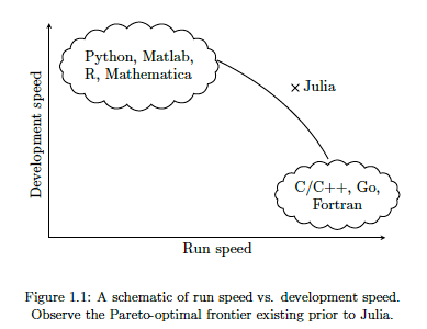
A (or not so) new language for data science and machine learning is Julia. Actually it has been around for a while now, and life began on it in 2009, whereas R (and S) and Python have their beginnings back in the 1980’s and early 1990’s. Does that make them legacy programming languages? or it just took a bit of time to mature and gain popularity?
There are lots of advantages to Julia, just like there are lots of advantages with the other languages. The following diagram illustrates one of the core advantages of Julia, it isn’t an interpreted language like R and Python, which means Julia will be significantly faster, yet still allows interactive development using Notebooks, just like R and Python. Julia was designed and build for data science and machine learning, and is designed for scale which makes it a good fit for MLOps. The list of advantages and differences can go on a bit and those are not the point of this post.
The remainder of this post will step through what is needed to get Julia working with an Oracle Database, and you have setup an IDE. Check out the Julia website for excellent installation instructions and selecting an IDE. If you coming from an R and/or Python background, using Jupyter Notebooks is a good option, and as you become more experienced there are a number of more advanced IDEs available for you to use. I’m assuming you have installed Julia.
If you have done a new install of Julia, make sure to add the install directory to the search PATH.
First Download load and install Oracle Instant Client. This is needed by the Julia packages to communicate with Oracle Database. After installing make sure to setup the following in your environment (environment variables and Path)
- ORACLE_HOME : points to where you installed Oracle Instant Client
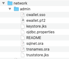
- TNS_ADMIN : points to the directory containing the wallet/tnsnames files. This will be a sub-directory in Oracle Instant Client directory, for example, it points to …/instantclient_19_8/network/admin
- PATH : include the Oracle Instant Client install directory in the PATH.
Next step is to setup the Oracle Client network files. As your DBA for the tnsnames.ora file or for the Wallet Zip file for your database. The Wallet Zip file is the most common approach. Unzip this Wallet file and copy the unzipped files to the TNS_ADMIN directory. See the second bullet point above to for this (…/instantclient_19_8/network/admin).
That’s all you need to do on the Oracle setup. I’m assuming you have a username and password for the Oracle Database you will be using.
Now we can setup Julia to use the Oracle Instant Client software. It is important you have setup those environment variables l’ve listed above.
There is an Oracle.jl package, developed by Felipe Noronha, which runs on top of Oracle Instant Client. To install this, load the Pkg package then then add the Oracle package. The following shows these commands and part of the output from the installation.
julia> using Pkg

julia> Pkg.add("Oracle")
Updating registry at `~/.julia/registries/General`
######################################################################## 100.0%
Resolving package versions...
Installed Reexport ──────────────────── v1.0.0
Installed libsodium_jll ─────────────── v1.0.18+1
Installed Compat ────────────────────── v3.25.0
Installed OrderedCollections ────────── v1.3.3
Installed WebSockets ────────────────── v1.5.9
Installed JuliaInterpreter ──────────── v0.8.8
Installed DataStructures ────────────── v0.18.9
Installed DataAPI ───────────────────── v1.5.1
Installed Requires ──────────────────── v1.1.2
Installed DataValueInterfaces ───────── v1.0.0
Installed Parsers ───────────────────── v1.0.15
Installed FlameGraphs ───────────────── v0.2.5
Installed URIs ──────────────────────── v1.2.0
Installed Colors ────────────────────── v0.12.6
Installed Oracle ────────────────────── v0.2.0
...
...
...
[7240a794] + Oracle v0.2.0
[bac558e1] ↑ OrderedCollections v1.3.2 ⇒ v1.3.3
[69de0a69] ↑ Parsers v1.0.12 ⇒ v1.0.15
[189a3867] ↑ Reexport v0.2.0 ⇒ v1.0.0
[ae029012] ↑ Requires v1.1.1 ⇒ v1.1.2
[3783bdb8] + TableTraits v1.0.0
[bd369af6] + Tables v1.3.2
[0796e94c] ↑ Tokenize v0.5.8 ⇒ v0.5.13
[5c2747f8] + URIs v1.2.0
[104b5d7c] ↑ WebSockets v1.5.2 ⇒ v1.5.9
[8f1865be] ↑ ZeroMQ_jll v4.3.2+5 ⇒ v4.3.2+6
[a9144af2] + libsodium_jll v1.0.18+1
Building Oracle → `~/.julia/packages/Oracle/CEOWz/deps/build.log`

julia>
You are now ready to load this Oracle package and use it to connect to an Oracle Database. Setting up a connection is really simple and in the following example I’m connecting to an ATP Database on Oracle Free Tier. The following sets up some variables, creates a connection, prints a statement and connection information and then closes the connection.
import Oracle

username="oml_user"
password="xxxxxxxxxxx"
dbname="yyyyyyyyyyyy"

conn = Oracle.Connection(username, password, dbname)

println("Connected")
println(conn)

Oracle.close(conn)
Job done 🙂
There is little additional connection information available. To test the connection a bit more let’s list what tables I have in my test/demo schema/user.
import Oracle

username="oml_user"
password="xxxxxxxxxxx"
dbname="yyyyyyyyyyyy"

conn = Oracle.Connection(username, password, dbname)

println("Tables")
println("--------------------")

Oracle.query(conn, "SELECT table_name FROM user_tables") do cursor
    for row in cursor
    # row values can be accessed using column name or position
        println( row["TABLE_NAME"] ) # same as row[1]
    end
end

println("")
println("...the end...")

Oracle.close(conn)
If you come from a Python background the syntax is familiar which makes the move other to Julia an easier task.
One other difference is, running the above code does seem to run a lot quicker in Julia. I haven’t measured it and the difference is less than a second but it is noticeable. For me, the above code generate the following output,
Tables
--------------------
WINE
BANK_ADDITIONAL_FULL
MINING_DATA_BUILD_V

...the end...
I’ll have additional posts looking are difference aspects and commands for working with and processing data in an Oracle Database.
2020 Books on Data Science and Machine Learning
2020 has been an interesting year. Not for the obvious topic, but for new books on Data Science and Machine Learning. The list below are some of my favorite books from 2020. Making the selection was difficult. Some months had a large number of releases and some were a bit quieter. The books below are listed based on their release date and are not ranked in any way. I’ve included links to these books on Amazon (.com, .uk and .de).
 |
 |
 |
|
| January
Everyone wants to work in Data Science, but where and how do you start. Aimed at beginners with guidance without the technical. High level, not for everyone. |
February
Taking ML to the next stage creating AI application. How to do it with examples across a number of areas. |
March
A guide for those wary of impact of technology’s and for those who are enthusiastic about where AI is taking us. |
|
 |
 |
 |
|
| April
AI Ethics was one of the topic topics for 2020. Covers the philosophical aspects along with the technical one.s |
May
Covering the life-cyle of building ML application, showing all that it entails and how ML plays a small part in the overall solution |
June
From covering the basics of NLP, it builds on this to include in application, how to use in different industries and within project teams. |
|
 |
 |
 |
|
| July
With by Thomas Davenport and others, and is a good addition to his other books. Consisting of interviews, research and analysis on how to win with ML & AI. |
August
I was invited to contribute a couple of chapters to this book, along with well known names in areas of DS, ML & AI |
September
Building upon the success of their 1st edition, the 2nd edition comes with more example and extra chapters. |
|
 |
 |
 |
|
| October
ML & AI is not perfect. Lots can go wrong. Not just with the project but also with the implementation of the applications. Lots to thing about and consider. |
November
No one really builds ML algorithms. We build ML solutions and applications. But whats the best way to do this, from technical, organizational and ethical aspects. |
December
It was difficult to pick a book for this month. Lots of new releases and I haven’t received all my orders, at time of this post. Here is a book from July, and is related to an Automated Trading App I’ve been working on (and earning) for a couple of years. |
And to finish off the list I’m including this additional book. It wasn’t released this year. It was released in April 2018. It was a best seller on Amazon in 2018 and 2019! This was really exciting for us and we still amazed at how it it is still selling in 2020. It is currently, as of December 2020, listed in 8th place on the MIT Press Best Sellers list. It won’t be making any best seller list in 2020, but is still proving popular with many readers. To all of you who have bought this book, I’d like to say Thank You and wishing you all the best with 2021 and beyond.
Adding Text Processing to Classification Machine Learning in Oracle Machine Learning
One of the typical machine learning functions is Classification. This is in widespread use across most domains and geographic regions. I’ve written several blog posts on this topic over many years (and going back many, many year) on how to do this using Oracle Machine Learning (OML) (formally known as Oracle Advanced Analytic and in the Oracle Data Miner tool in SQL Developer). Just do a quick search of my blog to find some of these posts.
When it comes to Classification problems, typically the data set will be contain your typical categorical and numerical variables/features. The Automatic Data Preparation (ADP) feature of OML where it automatically pre-processes and transforms these variable for input to the machine learning algorithm. This greatly reduces the boring work of the data scientist and increases their productivity.
But sometimes data sets come with text descriptions. These will contain production descriptions, free format text, and other descriptive data, for example product reviews. But how can this information be included as part of the input data set to the machine learning algorithms. Oracle allows this kind of input data, and a letting bit of setup is needed to tell Oracle how to process the data set. This uses the in-database feature of Oracle Text.
The following example walks through an example of the steps needed to pre-process and include the text processing as part of the machine learning algorithm.
The data set: The data used to illustrate this and to show the steps needed, is a data set from Kaggle webiste. This data set contains 130K Wine Reviews. This data set contain descriptive information of the wine with attributes about each wine including country, region, number of points, price, etc as well as a text description contain a review of the wine.
The following are 2 files containing the DDL (to create the table) and then Import the data set (using sql script with insert statements). These can be run in your schema (in order listed below).
I’ll leave the Data Exploration to you to do and to discover some early insights.
The ML Question
I want to be able to predict if a wine is a good quality wine, based on the prices and different characteristics of the wine?
Data Preparation
To be able to answer this question the first thing needed is to define a target variable to identify good and bad wines. To do this create a new attribute/feature called POINTS_BIN and populate it based on the number of points a wine has. If it has >90 points it is a good wine, if <90 points it is a bad wine.
ALTER TABLE WineReviews130K_bin ADD POINTS_BIN VARCHAR2(15);

UPDATE WineReviews130K_bin
SET POINTS_BIN = 'GT_90_Points'
WHERE winereviews130k_bin.POINTS >= 90;

UPDATE WineReviews130K_bin
SET POINTS_BIN = 'LT_90_Points'
WHERE winereviews130k_bin.POINTS < 90;

alter table WineReviews130K_bin DROP COLUMN POINTS;
The DESCRIPTION column data type needs to be changed to CLOB. This is to allow the Text Mining feature to work correctly.
-- add a new column of data type CLOB
ALTER TABLE WineReviews130K_bin ADD (DESCRIPTION_NEW CLOB);

-- update new column with data from the DESCRIPTION attribute
UPDATE WineReviews130K_bin SET DESCRIPTION_NEW = DESCRIPTION;

-- drop the DESCRIPTION attribute from table
ALTER TABLE WineReviews130K_bin DROP COLUMN DESCRIPTION;

-- rename the new attribute to replace DESCRIPTION
ALTER TABLE WineReviews130K_bin RENAME COLUMN DESCRIPTION_NEW TO DESCRIPTION;
Text Mining Configuration
There are a number of things we need to define for the Text Mining to work, these include a Lexer, Stop Word list and preferences.
First define the Lexer to use. In this case we will use a basic one and basic settings
BEGIN
   ctx_ddl.create_preference('mylex', 'BASIC_LEXER');
   ctx_ddl.set_attribute('mylex', 'printjoins', '_-');
   ctx_ddl.set_attribute ( 'mylex', 'index_themes', 'NO');
   ctx_ddl.set_attribute ( 'mylex', 'index_text', 'YES');
END;
Next we can define a Stop Word List. Oracle Text comes with a predefined set of Stop Word lists for most of the common languages. You can add to one of those list or create your own. Depending on the domain you are working in it might be easier to create your own and it is very straight forward to do. For example:
DECLARE
   v_stoplist_name varchar2(100);
BEGIN
   v_stoplist_name := 'mystop';
   ctx_ddl.create_stoplist(v_stoplist_name, 'BASIC_STOPLIST');
   ctx_ddl.add_stopword(v_stoplist_name, 'nonetheless');
   ctx_ddl.add_stopword(v_stoplist_name, 'Mr');
   ctx_ddl.add_stopword(v_stoplist_name, 'Mrs');
   ctx_ddl.add_stopword(v_stoplist_name, 'Ms');
   ctx_ddl.add_stopword(v_stoplist_name, 'a');
   ctx_ddl.add_stopword(v_stoplist_name, 'all');
   ctx_ddl.add_stopword(v_stoplist_name, 'almost');
   ctx_ddl.add_stopword(v_stoplist_name, 'also');
   ctx_ddl.add_stopword(v_stoplist_name, 'although');
   ctx_ddl.add_stopword(v_stoplist_name, 'an');
   ctx_ddl.add_stopword(v_stoplist_name, 'and');
   ctx_ddl.add_stopword(v_stoplist_name, 'any');
   ctx_ddl.add_stopword(v_stoplist_name, 'are');
   ctx_ddl.add_stopword(v_stoplist_name, 'as');
   ctx_ddl.add_stopword(v_stoplist_name, 'at');
   ctx_ddl.add_stopword(v_stoplist_name, 'be');
   ctx_ddl.add_stopword(v_stoplist_name, 'because');
   ctx_ddl.add_stopword(v_stoplist_name, 'been');
   ctx_ddl.add_stopword(v_stoplist_name, 'both');
   ctx_ddl.add_stopword(v_stoplist_name, 'but');
   ctx_ddl.add_stopword(v_stoplist_name, 'by');
   ctx_ddl.add_stopword(v_stoplist_name, 'can');
   ctx_ddl.add_stopword(v_stoplist_name, 'could');
   ctx_ddl.add_stopword(v_stoplist_name, 'd');
   ctx_ddl.add_stopword(v_stoplist_name, 'did');
   ctx_ddl.add_stopword(v_stoplist_name, 'do');
   ctx_ddl.add_stopword(v_stoplist_name, 'does');
   ctx_ddl.add_stopword(v_stoplist_name, 'either');
   ctx_ddl.add_stopword(v_stoplist_name, 'for');
   ctx_ddl.add_stopword(v_stoplist_name, 'from');
   ctx_ddl.add_stopword(v_stoplist_name, 'had');
   ctx_ddl.add_stopword(v_stoplist_name, 'has');
   ctx_ddl.add_stopword(v_stoplist_name, 'have');
   ctx_ddl.add_stopword(v_stoplist_name, 'having');
   ctx_ddl.add_stopword(v_stoplist_name, 'he');
   ctx_ddl.add_stopword(v_stoplist_name, 'her');
   ctx_ddl.add_stopword(v_stoplist_name, 'here');
   ctx_ddl.add_stopword(v_stoplist_name, 'hers');
   ctx_ddl.add_stopword(v_stoplist_name, 'him');
   ctx_ddl.add_stopword(v_stoplist_name, 'his');
   ctx_ddl.add_stopword(v_stoplist_name, 'how');
   ctx_ddl.add_stopword(v_stoplist_name, 'however');
   ctx_ddl.add_stopword(v_stoplist_name, 'i');
   ctx_ddl.add_stopword(v_stoplist_name, 'if');
   ctx_ddl.add_stopword(v_stoplist_name, 'in');
   ctx_ddl.add_stopword(v_stoplist_name, 'into');
   ctx_ddl.add_stopword(v_stoplist_name, 'is');
   ctx_ddl.add_stopword(v_stoplist_name, 'it');
   ctx_ddl.add_stopword(v_stoplist_name, 'its');
   ctx_ddl.add_stopword(v_stoplist_name, 'just');
   ctx_ddl.add_stopword(v_stoplist_name, 'll');
   ctx_ddl.add_stopword(v_stoplist_name, 'me');
   ctx_ddl.add_stopword(v_stoplist_name, 'might');
   ctx_ddl.add_stopword(v_stoplist_name, 'my');
   ctx_ddl.add_stopword(v_stoplist_name, 'no');
   ctx_ddl.add_stopword(v_stoplist_name, 'non');
   ctx_ddl.add_stopword(v_stoplist_name, 'nor');
   ctx_ddl.add_stopword(v_stoplist_name, 'not');
   ctx_ddl.add_stopword(v_stoplist_name, 'of');
   ctx_ddl.add_stopword(v_stoplist_name, 'on');
   ctx_ddl.add_stopword(v_stoplist_name, 'one');
   ctx_ddl.add_stopword(v_stoplist_name, 'only');
   ctx_ddl.add_stopword(v_stoplist_name, 'onto');
   ctx_ddl.add_stopword(v_stoplist_name, 'or');
   ctx_ddl.add_stopword(v_stoplist_name, 'our');
   ctx_ddl.add_stopword(v_stoplist_name, 'ours');
   ctx_ddl.add_stopword(v_stoplist_name, 's');
   ctx_ddl.add_stopword(v_stoplist_name, 'shall');
   ctx_ddl.add_stopword(v_stoplist_name, 'she');
   ctx_ddl.add_stopword(v_stoplist_name, 'should');
   ctx_ddl.add_stopword(v_stoplist_name, 'since');
   ctx_ddl.add_stopword(v_stoplist_name, 'so');
   ctx_ddl.add_stopword(v_stoplist_name, 'some');
   ctx_ddl.add_stopword(v_stoplist_name, 'still');
   ctx_ddl.add_stopword(v_stoplist_name, 'such');
   ctx_ddl.add_stopword(v_stoplist_name, 't');
   ctx_ddl.add_stopword(v_stoplist_name, 'than');
   ctx_ddl.add_stopword(v_stoplist_name, 'that');
   ctx_ddl.add_stopword(v_stoplist_name, 'the');
   ctx_ddl.add_stopword(v_stoplist_name, 'their');
   ctx_ddl.add_stopword(v_stoplist_name, 'them');
   ctx_ddl.add_stopword(v_stoplist_name, 'then');
   ctx_ddl.add_stopword(v_stoplist_name, 'there');
   ctx_ddl.add_stopword(v_stoplist_name, 'therefore');
   ctx_ddl.add_stopword(v_stoplist_name, 'these');
   ctx_ddl.add_stopword(v_stoplist_name, 'they');
   ctx_ddl.add_stopword(v_stoplist_name, 'this');
   ctx_ddl.add_stopword(v_stoplist_name, 'those');
   ctx_ddl.add_stopword(v_stoplist_name, 'though');
   ctx_ddl.add_stopword(v_stoplist_name, 'through');
   ctx_ddl.add_stopword(v_stoplist_name, 'thus');
   ctx_ddl.add_stopword(v_stoplist_name, 'to');
   ctx_ddl.add_stopword(v_stoplist_name, 'too');
   ctx_ddl.add_stopword(v_stoplist_name, 'until');
   ctx_ddl.add_stopword(v_stoplist_name, 've');
   ctx_ddl.add_stopword(v_stoplist_name, 'very');
   ctx_ddl.add_stopword(v_stoplist_name, 'was');
   ctx_ddl.add_stopword(v_stoplist_name, 'we');
   ctx_ddl.add_stopword(v_stoplist_name, 'were');
   ctx_ddl.add_stopword(v_stoplist_name, 'what');
   ctx_ddl.add_stopword(v_stoplist_name, 'when');
   ctx_ddl.add_stopword(v_stoplist_name, 'where');
   ctx_ddl.add_stopword(v_stoplist_name, 'whether');
   ctx_ddl.add_stopword(v_stoplist_name, 'which');
   ctx_ddl.add_stopword(v_stoplist_name, 'while');
   ctx_ddl.add_stopword(v_stoplist_name, 'who');
   ctx_ddl.add_stopword(v_stoplist_name, 'whose');
   ctx_ddl.add_stopword(v_stoplist_name, 'why');
   ctx_ddl.add_stopword(v_stoplist_name, 'will');
   ctx_ddl.add_stopword(v_stoplist_name, 'with');
   ctx_ddl.add_stopword(v_stoplist_name, 'would');
   ctx_ddl.add_stopword(v_stoplist_name, 'yet');
   ctx_ddl.add_stopword(v_stoplist_name, 'you');
   ctx_ddl.add_stopword(v_stoplist_name, 'your');
   ctx_ddl.add_stopword(v_stoplist_name, 'yours');
   ctx_ddl.add_stopword(v_stoplist_name, 'drink');
   ctx_ddl.add_stopword(v_stoplist_name, 'flavors');
   ctx_ddl.add_stopword(v_stoplist_name, '2020');
   ctx_ddl.add_stopword(v_stoplist_name, 'now');
END;
Next define the preferences for processing the Text, for example what Stop Word list to use, if Fuzzy match is to be used and what language to use for this, number of tokens/words to process and if stemming is to be used.
BEGIN
   ctx_ddl.create_preference('mywordlist', 'BASIC_WORDLIST');
   ctx_ddl.set_attribute('mywordlist','FUZZY_MATCH','ENGLISH');
   ctx_ddl.set_attribute('mywordlist','FUZZY_SCORE','1');
   ctx_ddl.set_attribute('mywordlist','FUZZY_NUMRESULTS','5000');
   ctx_ddl.set_attribute('mywordlist','SUBSTRING_INDEX','TRUE');
   ctx_ddl.set_attribute('mywordlist','STEMMER','ENGLISH');
END;
And the final step is to piece it all together by defining a new Text policy
BEGIN
   ctx_ddl.create_policy('my_policy', NULL, NULL, 'mylex', 'mystop', 'mywordlist');
END;
Define Settings for OML Model
We will create two models. An Attribute Importance model and a Classification model. The following defines the model parameters for each of these.
CREATE TABLE att_import_model_settings (setting_name varchar2(30), setting_value varchar2(30));
INSERT INTO att_import_model_settings (setting_name, setting_value)
VALUES (''ALGO_NAME'', ''ALGO_AI_MDL'');
INSERT INTO att_import_model_settings (setting_name, setting_value)
VALUES (''PREP_AUTO'', ''ON'');
INSERT INTO att_import_model_settings (setting_name, setting_value)
VALUES (''ODMS_TEXT_POLICY_NAME'', ''my_policy'');
INSERT INTO att_import_model_settings (setting_name, setting_value)
VALUES (''ODMS_TEXT_MAX_FEATURES'', ''3000'')';
CREATE TABLE wine_model_settings (setting_name varchar2(30), setting_value varchar2(30));
INSERT INTO wine_model_settings (setting_name, setting_value)
VALUES (''ALGO_NAME'', ''ALGO_RANDOM_FOREST'');
INSERT INTO wine_model_settings (setting_name, setting_value)
VALUES (''PREP_AUTO'', ''ON'');
INSERT INTO wine_model_settings (setting_name, setting_value)
VALUES (''ODMS_TEXT_POLICY_NAME'', ''my_policy'');
INSERT INTO wine_model_settings (setting_name, setting_value)
VALUES (''ODMS_TEXT_MAX_FEATURES'', ''3000'')';
Create the Training and Test data sets.
CREATE TABLE wine_train_data
AS SELECT id, country, description, designation, points_bin, price, province, region_1, region_2, taster_name, variety, title
FROM winereviews130k_bin
SAMPLE (60) SEED (1);
CREATE TABLE wine_test_data
AS SELECT id, country, description, designation, points_bin, price, province, region_1, region_2, taster_name, variety, title
FROM winereviews130k_bin
WHERE id NOT IN (SELECT id FROM wine_train_data);
All the set up is done, we can move onto the creating the machine learning models.
Create the OML Model (Attribute Importance & Classification)
We are going to create two models. The first is an Attribute Important model. This will look at the data set and will determine what attributes contribute most towards determining the target variable. As we are incorporting Texting Mining we will see what words/tokens from the DESCRIPTION attribute also contribute towards the target variable.
BEGIN
   DBMS_DATA_MINING.CREATE_MODEL(
      model_name          => 'GOOD_WINE_AI',
      mining_function     => DBMS_DATA_MINING.ATTRIBUTE_IMPORTANCE,
      data_table_name     => 'winereviews130k_bin',
      case_id_column_name => 'ID',
      target_column_name  => 'POINTS_BIN',
      settings_table_name => 'att_import_mode_settings');
END;
We can query the system views for Oracle ML to find out what are the important variables.
SELECT * FROM dm$vagood_wine_ai
ORDER BY attribute_rank;
Here is the listing of the top 15 most important attributes. We can see from the first 15 rows and looking under column ATTRIBUTE_SUBNAME, the words from the DESCRIPTION attribute that seem to be important and contribute towards determining the value in the target attribute.

At this point you might determine, based on domain knowledge, some of these words should be excluded as they are generic for the domain. In this case, go back to the Stop Word List and recreate it with any additional words. This can be repeated until you are happy with the list. In this example, WINE could be excluded by including it in the Stop Word List.
Run the following to create the Classification model. It is very similar to what we ran above with minor changes to the name of the model, the data mining function and the name of the settings table.
BEGIN
   DBMS_DATA_MINING.CREATE_MODEL(
      model_name          => 'GOOD_WINE_MODEL',
      mining_function     => DBMS_DATA_MINING.CLASSIFICATION,
      data_table_name     => 'winereviews130k_bin',
      case_id_column_name => 'ID',
      target_column_name  => 'POINTS_BIN',
      settings_table_name => 'wine_model_settings');
END;
Apply OML Model
The model can be applied in similar ways to any other ML model created using OML. For example the following displays the wine details along with the predicted points bin values (good or bad) and the probability score (<=1) of the prediction.
SELECT id, price, country, designation, province, variety, points_bin,
       PREDICTION(good_wine_mode USING *) pred_points_bin,
       PREDICTION_PROBABILITY(good_wine_mode USING *) prob_points_bin
FROM wine_test_data;
Pre-build Machine Learning Models
Machine learning has seen widespread adoption over the past few years. In more recent times we have seem examples of how the models, created by the machine learning algorithms, can be shared. There have been various approaches to sharing these models using different model interchange languages. Some of these have become more or less popular over time, for example a few years ago PMML was very popular, and in more recent times ONNX seems to popular. Who knows what it will be next year or in a couple of years time.
With the increased use of machine learning models and the ability to share them, we are now seeing other uses of them. Typically the sharing of models involved a company transferring a model developed by the data scientists in their lab environment, to DevOps teams who then deploy the model into the production environment. This has developed a new are of expertise of MLOps or AIOps.
The languages and tools used by the data scientists in the lab environment are different to the languages used to deploy applications in production. The model interchange languages can be used take the model parameters, algorithm type and data transformations, etc and map these into the interchange language. The production environment would read this interchange object and apply it to the production language. In such situations the models will use the algorithms already coded in the production language. For example, the lab environment could be using Python. But the product environment could be using C, Java, Go, etc. Python is an interpretative language and in a lot of cases is not suitable for real-time use in a production environment, due to speed and scalability issues. In this case the underlying algorithm of the production language will be used and not algorithm used in the lab. In theory the algorithms should be the same. For example a decision tree algorithm using Gini Index in one language should function in the same way in another language. We all know there can be a small to a very large difference between what happens in theory and how it works in practice. Different language and different developers will do things slightly differently. This means there will be differences between the accuracy of the models developed in the lab versus the accuracy of the (same) model used in production. As long as everyone is aware of this, then everything will be ok. But it will be important task, for the data science team, to have some measurements of these differences.

Moving on a little this a little, we are now seeing some other developments with the development and sharing of machine learning models, and the use of these open model interchange languages, like ONNX, makes this possible.
We are now seeing people making their machine learning models available to the wider community, instead of keeping them within their own team or organization.
Why would some one do this? why would they share their machine learning model? It’s a bit like the picture to the left which comes from a very popular kids programme on the BBC called Blue Peter. They would regularly show some craft projects for kids to work on at home. They would never show all the steps needed to finish the project and would end up showing us “one I made earlier”. It always looked perfect and nothing like what they tried to make in the studio and nothing like my attempt.
But having pre-made machine learning models is now a thing. There ware lots of examples of these and for example the ONNX website has several pre-trained models ready for you to use. These cover various examples for image classification, object detection, machine translation and comprehension, language modeling, speech and audio processing, etc. More are being added over time.
Most of these pre-trained models are based on defined data sets and problems and allows others to see what they have done, and start building upon their work without the need to go through the training and validating phase.
Could we have something like this in the commercial world? Could we have pre-trained machine learning models being standardized and shared across different organizations? Again the in-theory versus in-practical terms apply. Many organizations within a domain use the same or similar applications for capturing, storing, processing and analyzing their data. In this case could the sharing of machine learning models help everyone be more competitive or have better insights and discoveries from their data? Again the difference between in-theory versus in-practice applies.
Some might remember in the early days of Data Warehousing we used to have some industry (dimensional) models, and vendors and consulting companies would offer their custom developed industry models and how to populate these. In theory these were supposed to help companies to speed up their time to data insights and save money. We have seem similar attempts at doing similar things over the decades. But the reality was most projects ended up being way more expensive and took way too long to deploy due to lots of technical difficulties and lots of differences in the business understand, interpretation and deployment of the underlying applications. The pre-built DW model was generic and didn’t really fit in with the business needs.
Although we are seeing more and more pre-trained machine learning models appearing on the market. Many vendors are offering pre-trained solutions. But can these really work. Some of these pre-trained models are based on certain data preparation, using one particular machine learning model and using only one particular evaluation matric. As with the custom DW models of twenty years ago, pre-trained ML models are of limited use.
Everyone is different, data is different, behavior is different, etc. the list goes on. Using the principle of the “No Free Lunch” theorem, although we might be using the same or similar applications for capturing, storing, processing and analysing their data, the underlying behavior of the data (and the transactions, customers etc that influence that), will be different, the marketing campaigns will be different, business semantics may be different, general operating models will be different, etc. Based on “No Free Lunch” we need to explore the data using a variety of different algorithms, to determine what works for our data at this point in time. The behavior of the data (and business influences on it) keep on changing and evolving on a daily, weekly, monthly, etc basis. A great example of this but in a more extreme and rapid rate of change happened during the COVID pandemic. Most of the machine learning models developed over the preceding period no longer worked, the models developed during the pandemic have a very short life span, and it will take some time before “normal” will return and newer models can be built to represent the “new normal”
Principal Component Analysis (PCA) in Oracle
Principal Component Analysis (PCA), is a statistical process used for feature or dimensionality reduction in data science and machine learning projects. It summarizes the features of a large data set into a smaller set of features by projecting each data point onto only the first few principal components to obtain lower-dimensional data while preserving as much of the data’s variation as possible. There are lots of resources that goes into the mathematics behind this approach. I’m not going to go into that detail here and a quick internet search will get you what you need.
PCA can be used to discover important features from large data sets (large as in having a large number of features), while preserving as much information as possible.
Oracle has implemented PCA using Sigular Value Decomposition (SVD) on the covariance and correlations between variables, for feature extraction/reduction. PCA is closely related to SVD. PCA computes a set of orthonormal bases (principal components) that are ranked by their corresponding explained variance. The main difference between SVD and PCA is that the PCA projection is not scaled by the singular values. The extracted features are transformed features consisting of linear combinations of the original features.
When machine learning is performed on this reduced set of transformed features, it can completed with less resources and time, while still maintaining accuracy.
Algorithm Name in Oracle using
Mining Model Function = FEATURE_EXTRACTION
Algorithm = ALGO_SINGULAR_VALUE_DECOMP
(Hyper)-Parameters for algorithms
- SVDS_U_MATRIX_OUTPUT : SVDS_U_MATRIX_ENABLE or SVDS_U_MATRIX_DISABLE
- SVDS_SCORING_MODE : SVDS_SCORING_SVD or SVDS_SCORING_PCA
- SVDS_SOLVER : possible values include SVDS_SOLVER_TSSVD, SVDS_SOLVER_TSEIGEN, SVDS_SOLVER_SSVD, SVDS_SOLVER_STEIGEN
- SVDS_TOLERANCE : range of 0…1
- SVDS_RANDOM_SEED : range of 0…4294967296 (!)
- SVDS_OVER_SAMPLING : range of 1…5000
- SVDS_POWER_ITERATIONS : Default value 2, with possible range of 0…20
Let’s work through an example using the MINING_DATA_BUILD_V data set that comes with Oracle Data Miner.
First step is to define the parameter settings for the algorithm. No data preparation is needed as the algorithm takes care of this. This means you can disable the Automatic Data Preparation (ADP).
-- create the parameter table
CREATE TABLE svd_settings (
setting_name VARCHAR2(30),
setting_value VARCHAR2(4000));

-- define the settings for SVD algorithm
BEGIN
   INSERT INTO svd_settings (setting_name, setting_value)
   VALUES (dbms_data_mining.algo_name, dbms_data_mining.algo_singular_value_decomp);

   -- turn OFF ADP
   INSERT INTO svd_settings (setting_name, setting_value)
   VALUES (dbms_data_mining.prep_auto, dbms_data_mining.prep_auto_off);

   -- set PCA scoring mode
   INSERT INTO svd_settings (setting_name, setting_value)
   VALUES (dbms_data_mining.svds_scoring_mode, dbms_data_mining.svds_scoring_pca);

   INSERT INTO svd_settings (setting_name, setting_value)
   VALUES (dbms_data_mining.prep_shift_2dnum, dbms_data_mining.prep_shift_mean);

   INSERT INTO svd_settings (setting_name, setting_value)
   VALUES (dbms_data_mining.prep_scale_2dnum, dbms_data_mining.prep_scale_stddev);
END;
/
You are now ready to create the model.
BEGIN
   DBMS_DATA_MINING.CREATE_MODEL(
      model_name          => 'SVD_MODEL',
      mining_function     => dbms_data_mining.feature_extraction,
      data_table_name     => 'mining_data_build_v',
      case_id_column_name => 'CUST_ID',
      settings_table_name => 'svd_settings');
END;
When created you can use the mining model data dictionary views to explore the model and to explore the specifics of the model and the various MxN matrix created using the model specific views. These include:
- DM$VESVD_Model : Singular Value Decomposition S Matrix
- DM$VGSVD_Model : Global Name-Value Pairs
- DM$VNSVD_Model : Normalization and Missing Value Handling
- DM$VSSVD_Model : Computed Settings
- DM$VUSVD_Model : Singular Value Decomposition U Matrix
- DM$VVSVD_Model : Singular Value Decomposition V Matrix
- DM$VWSVD_Model : Model Build Alerts
Where the S, V and U matrix contain:
- U matrix : consists of a set of ‘left’ orthonormal bases
- S matrix : is a diagonal matrix
- V matrix : consists of set of ‘right’ orthonormal bases
These can be explored using the following
-- S matrix
select feature_id, VALUE, variance, pct_cum_variance
from DM$VESVD_MODEL;

-- V matrix
select feature_id, attribute_name, value
from DM$VVSVD_MODEL
order by feature_id, attribute_name;

-- U matrix
select feature_id, attribute_name, value
from DM$VVSVD_MODEL
order by feature_id, attribute_name;
To determine the projections to be used for visualizations we can use the FEATURE_VALUES function.
select FEATURE_VALUE(svd_sh_sample, 1 USING *) proj1,
       FEATURE_VALUE(svd_sh_sample, 2 USING *) proj2
from   mining_data_build_v
where  cust_id <= 101510
order by 1, 2;
Other algorithms available in Oracle for feature extraction and reduction include:
- Non-Negative Matrix Factorization (NMF)
- Explicit Semantic Analysis (ESA)
- Minimum Description Length (MDL) – this is really feature selection rather than feature extraction
ONNX for exchanging Machine Learning Models
When working on build predictive application using machine learning algorithms, you will probably be working with such languages as Python, R, PyTorch, TensorFlow, and lots of other frameworks. One of the challenges we face is taking these machine learning models from our test/lab environment and putting into production them. By this I mean integrating them with our production systems to allow real-time use of these ML models. This is not a topic that is discussed very often. Many of the most common languages and frameworks are very easy to use for machine learning, but running them in production can be slow. This can lead to lots of problems and can regularly label machine learning projects as a failure. None of use want that. Sometime people look are re-coding all the machine learning models in other languages such as C or Java or Julia, as these are noted for the high speed and scalability in production environments. (Remember many of the common ML languages and frameworks are actually developed using C and Java.)
To remove the need to recode your models, many of the languages, frameworks and tools have opened to the ability to allow model interchange. This approach allows you to use the tools that work best for you, in your environment and your company, to develop, test and evaluate machine learning models. These can then be packaged up and shared with other languages, frameworks or tools suitable for production environments, eliminating or significantly reducing the need for large coding projects and allows for quicker time to deployment.
There are many machine learning model interchange frameworks available. Historically PMML was popular but with the rise of other machine learning and deep learning algorithms, it seems to have lost the popularity contest. One of the more popular machine learning interchange frameworks is called ONNX. This has been growing in popularity with a wide body of languages, tools and vendors.

ONNX stands for the Open Neural Network eXchange and is designed to allow developers to easily move between different machine learning and deep learning frameworks. This allows the easy migration from research and model development environments, to other environments more suited to deployment, allowing for faster scoring of data. ONNX allows for the migration of the model with the minimum of recoding. ONNX generates or provides for an extensible computation dataflow graph model, with built-in operators and data types focused on interencing.
To use ONNX with Python install the library:
pip3 install onnx-mxnetThe following is an extract of sample code generating a model, converting it to ONNX format and saving it to file.
#train a model
#load sklearn
from sklearn.datasets import load_iris
from sklearn.model_selection import train_test_split
from sklearn.ensemble import RandomForestClassifier

#load the IRIS sample data set
iris = load_iris()
X, y = iris.data, iris.target
#create the train and test data sets
X_train, X_test, y_train, y_test = train_test_split(X, y)
#define and create Random Forest data set
rf = RandomForestClassifier()
rf.fit(X_train, y_train)

#convert into ONNX format & save to file
from skl2onnx import convert_sklearn
from skl2onnx.common.data_types import FloatTensorType
initial_type = [('float_input', FloatTensorType([None, 4]))]
#covert to ONNX
onx = convert_sklearn(rf, initial_types=initial_type)
#save to file
with open("rf_iris.onnx", "wb") as f:
    f.write(onx.SerializeToString())
The above example illustrates converting a sklearn model. For algorithms and models, converters exist and are available in the ONNX Github
Adam Solver for Neural Networks (OML) in Oracle 21c
Updated: Changed 20c to Oracle 21c, as Oracle 20c Database never really existed 🙂
The ability to create and use Neural Networks on business data has been available in Oracle Database since Oracle 18c (18c and 19c are just slightly extended versions of Oracle 12c). With each minor database release we get some small improvements and minor features added. I’ve written other blog posts about other 21c new machine learning features (see here, here and here).
With Oracle 21c they have added a new neural network solver. This is called Adam Solver and the original research was conducted by Diederik Kingma from OpenAI and Jimmy Ba from the University of Toronto and they presented they work at ICLR 2015. The name Adam is derived from ‘adaptive moment estimation‘. This algorithm, research and paper has gathered some attention in the research community over the past few years. Most of this has been focused on the benefits of using it.

But care is needed. As with most machine learning (and deep learning) algorithms, they work up to a point. They may be good on certain problems and input data sets, and then for others they may not be as good or as efficient at producing an optimal outcome. Although using this solver may be beneficial to your problem, using the concept of ‘No Free Lunch’, you will need to prove the solver is beneficial for your problem.
With Oracle Machine Learning there are two Optimization Solver available for the Neural Network algorithm. The default solver is call L-BFGS (Limited memory Broyden-Fletch-Goldfarb-Shanno). This is one of the most popular solvers in use in most algorithms. The is a limited version of BFGS, using less memory (hence the L in the name) This solver finds the descent direction and line search is used to find the appropriate step size. The solver searches for the optimal solution of the loss function to find the extreme value (maximum or minimum) of the loss (cost) function
The Adam Solver uses an extension to stochastic gradient descent. It uses the squared gradients to scale the learning rate and it takes advantage of momentum by using moving average of the gradient instead of gradient. This allows the solver to work quickly by seeing less data and can work well with larger data sets.
With Oracle Data Mining the Adam Solver has the following parameters.
- ADAM_ALPHA : Learning rate for solver. Default value is 0.001.
- ADAM_BATCH_ROWS : Number of rows per batch. Default value is 10,000
- ADAM_BETA1 : Exponential decay rate for 1st moment estimates. Default value is 0.9.
- ADAM_BETA2 : Exponential decay rate for the 2nd moment estimates. Default value is 0.99.
- ADAM_GRADIENT_TOLERANCE : Gradient infinity norm tolerance. Default value is 1E-9.
The parameters ADAM_ALPHA and ADAM_BATCH_ROWS can have an effect on the timing for the neural network algorithm to produce the model. Some exploration is needed to determine the optimal values for this parameters based on the size of the data set. For example having a larger value for ADAM_ALPHA results in a faster initial learning before the rates is updated. Small values than the default slows learning down during training.
To tell Oracle Machine Learning to use the Adam Solver the DMSSET_NN_SOLVER parameter needs to be set. The default setting for a neural network is DMSSET_NN_SOLVER_LGFGS. But to use the Adam solver set it to DMSSET_NN_SOLVER_ADAM.
The following is an example of setting the parameters for the Adam solver and creating a neural network.
BEGIN
   DELETE FROM BANKING_NNET_SETTINGS;

   INSERT INTO BANKING_NNET_SETTINGS (setting_name, setting_value)
   VALUES (dbms_data_mining.algo_name, dbms_data_mining.algo_neural_network);

   INSERT INTO BANKING_NNET_SETTINGS (setting_name, setting_value)
   VALUES (dbms_data_mining.prep_auto, dbms_data_mining.prep_auto_on);

   INSERT INTO BANKING_NNET_SETTINGS (setting_name, setting_value)
   VALUES (dbms_data_mining.nnet_nodes_per_layer, '20,10,6');

   INSERT INTO BANKING_NNET_SETTINGS (setting_name, setting_value)
   VALUES (dbms_data_mining.nnet_iterations, 10);

   INSERT INTO BANKING_NNET_SETTINGS (setting_name, setting_value)
   VALUES (dbms_data_mining.NNET_SOLVER, 'NNET_SOLVER_ADAM');
END;

The addition of the last parameter overrides the default solver for building a neural network model.
To build the model we can use the following.
DECLARE
   v_start_time TIMESTAMP;
BEGIN
   begin DBMS_DATA_MINING.DROP_MODEL('BANKING_NNET_72K_1'); exception when others then null; end;

   v_start_time := current_timestamp;
   DBMS_DATA_MINING.CREATE_MODEL(
      model_name.         => 'BANKING_NNET_72K_1',
      mining_function     => dbms_data_mining.classification,
      data_table_name     => 'BANKING_72K',
      case_id_column_name => 'ID',
      target_column_name  => 'TARGET',
      settings_table_name => 'BANKING_NNET_SETTINGS');

   dbms_output.put_line('Time take to create model = ' || to_char(extract(second from (current_timestamp-v_start_time))) || ' seconds.');
END;
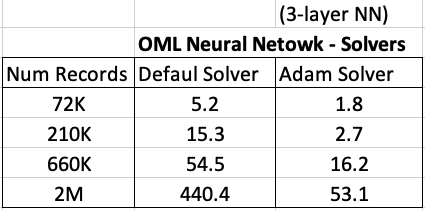
For me on my Oracle 20c Preview Database, this takes 1.8 seconds to run and create the neural network model ob a data set of 72,000 records.
Using the default solver, the model is created in 5.2 seconds. With using a small data set of 72,000 records, we can see the impact of using an Adam Solver for creating a neural network model.
These timings and the timings shown below (in seconds) are based on the Oracle 20c Preview Database, using a minimum VM sizing and specification available.
Creating OML Models in Parallel
In a previous post I showed how to use the partition option in Oracle Data Mining to create many sub-models. This gives one overall driving model with each sub-model created on a different subset or partition of the training data set.
That blog post also showed the timing for creating the models and how this compares to creating one overall model for your data set, while achieving greater accuracy with model predictions.
This is all good. But can it scale more. What if I have significantly more data! How does this scale and how?
My previous blog post showed how the you can quickly partition the data into different subsets and some care is needed on choosing the attributes carefully for the partition key.
What if I want to run these different sub-models on the different data partitions in parallel on different slaves.
This is simple to do and can be achieved by adding one additional parameter to the Model Settings table. This parameter is called ODMS_PARTITION_BUILD_TYPE. This parameter has three possible values:
ODMS_PARTITION_BUILD_INTRA — Each partition is built in parallel using all slaves.
ODMS_PARTITION_BUILD_INTER — Each partition is built entirely in a single slave, but multiple partitions may be built at the same time since multiple slaves are active.
ODMS_PARTITION_BUILD_HYBRID — It is a combination of the other two types and is recommended for most situations to adapt to dynamic environments.
The default mode is ODMS_PARTITION_BUILD_HYBRID.
Although by default the model will try to run in parallel, I’ve found this is not necessarily the case. In my previous post I showed the timing to create a model on 72K records using different models. These timings are
One over all Model = 5.23 seconds
Partitioned Model (4 partitions/models) = 8.3 seconds
Partitioned Model (48 partitions/models) = 37 seconds
Now let’s change/set the ODMS_PARTITION_BUILD_TYPE parameter. The following code is the complete code to set the parameters and build upon those shown in the previous blog post.
BEGIN
    DELETE FROM BANKING_RF_SETTINGS;

    INSERT INTO banking_RF_settings (setting_name, setting_value)
    VALUES (dbms_data_mining.algo_name, dbms_data_mining.algo_random_forest);

    INSERT INTO banking_RF_settings (setting_name, setting_value)
    VALUES (dbms_data_mining.prep_auto, dbms_data_mining.prep_auto_on);

    INSERT INTO banking_RF_settings (setting_name, setting_value)
    VALUES (dbms_data_mining.odms_partition_columns, 'MARITAL, JOB’);

    INSERT INTO banking_RF_settings (setting_name, setting_value)
    VALUES (dbms_data_mining.odms_partition_build_type, 'ODMS_PARTITION_BUILD_INTER');

   COMMIT;
END;
The code to create the Model using CREATE_MODEL does not change.
So, how long this this take to run? In my DBaaS preview 20c database (basic setup) it too 6.6 seconds.
Remember that was for an input data set consisting of 72K records and the partition key creates 48 partitions and in-turn creates 48 different machine learning models.
This 6.6 seconds compares to 37 seconds when this parameter was not set or using the default.
No that is fast and available to everyone to use 🙂
Partitioned Models – Oracle Machine Learning (OML)
Building machine learning models can be a relatively trivial task. But getting to that point and understanding what to do next can be challenging. Yes the task of creating a model is simple and usually takes a few line of code. This is what is shown in most examples. But when you try to apply to real world problems we are faced with other challenges. Some of which include volume of data is larger, building efficient ML pipelines is challenging, time to create models gets longer, applying models to new data in real-time takes longer (not possible in real-time), etc. Yes these are typically challenges and most of these can be easily overcome.
When building ML solutions for real-world problem you will be faced with building (and deploying) many 10s or 100s of ML models. Why are so many models needed? Almost every example we see for ML takes the entire data set and build a model on that data. When you think about it, not everyone in the data set can be considered in the same grouping (similar characteristics). If we were to build a model on the data set and apply it to new data, we will get a generic prediction. A prediction comparing the new data item (new customer, purchase, etc) with everyone else in the data population. Maybe this is why so many ML project fail as they are building generic solution that performs badly when run on new (and evolving) data.
To overcome this we start to look at the different groups of data in the data set. Can the data set be divided into a number of different parts based on some characteristics. If we could do this and build a separate model on each group (or cluster), then we would have ML models that would be more accurate with their predictions. This is where we will end up creating 10s or 100s of models. As you can imagine the work involved in doing this with be LOTs. Then think about all the coding needed to manage all of this. What about the complexity of all the code needed for making the predictions on new data.
Yes all of this gets complex very, very quickly!
Ideally we want a separate model for each group
But how can you do that efficiently? is it possible?
When working with Oracle Machine Learning, you can use a feature called partitioned models. Partitioned Models are designed to handle this type of problem. They are designed to:
- make the building of models simple
- scales as the data and number of partitions increase
- includes all the steps part of the ML pipeline (all the data prep, transformations, etc)
- make predicting new data using the ML model simple
- make the deployment of the ML model easy
- make the MLOps process simple
- make the use of ML model easy to use by all developers no matter the programming language
- make the ML model build and ML model scoring quick and with better, more accurate predictions.

Let us work through an example. In this example lets start by creating a Random Forest ML model using the entire data set. The following code shows setting up the Parameters settings table. The second code segment creates the Random Forest ML model. The training data set being used in this example contains 72,000 records.
BEGIN
  DELETE FROM BANKING_RF_SETTINGS;

  INSERT INTO banking_RF_settings (setting_name, setting_value)
  VALUES (dbms_data_mining.algo_name, dbms_data_mining.algo_random_forest);

  INSERT INTO banking_RF_settings (setting_name, setting_value)
  VALUES (dbms_data_mining.prep_auto, dbms_data_mining.prep_auto_on);

 COMMIT;
END;
/

-- Create the ML model
DECLARE
   v_start_time  TIMESTAMP;
BEGIN
   DBMS_DATA_MINING.DROP_MODEL('BANKING_RF_72K_1');

   v_start_time := current_timestamp;

   DBMS_DATA_MINING.CREATE_MODEL(
      model_name          => 'BANKING_RF_72K_1',
      mining_function     => dbms_data_mining.classification,
      data_table_name     => 'BANKING_72K',
      case_id_column_name => 'ID',
      target_column_name  => 'TARGET',
      settings_table_name => 'BANKING_RF_SETTINGS');

   dbms_output.put_line('Time take to create model = ' || to_char(extract(second from (current_timestamp-v_start_time))) || ' seconds.');
END;
/
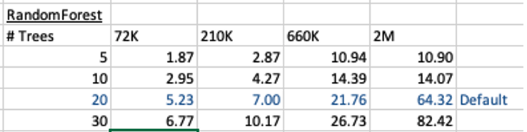
This is the basic setup and the following table illustrates how long the CREATE_MODEL function takes to run for different sizes of training datasets and with different number of trees per model. The default number of trees is 20.
To run this model against new data we could use something like the following SQL query.
SELECT cust_id, target,
       prediction(BANKING_RF_72K_1 USING *)  predicted_value,
       prediction_probability(BANKING_RF_72K_1 USING *) probability
FROM   bank_test_v;
This is simple and straight forward to use.
For the 72,000 records it takes just approx 5.23 seconds to create the model, which includes creating 20 Decision Trees. As mentioned earlier, this will be a generic model covering the entire data set.
To create a partitioned model, we can add new parameter which lists the attributes to use to partition the data set. For example, if the partition attribute is MARITAL, we see it has four different values. This means when this attribute is used as the partition attribute, Oracle Machine Learning will create four separate sub Random Forest models all until the one umbrella model. This means the above SQL query to run the model, does not change and the correct sub model will be selected to run on the data based on the value of MARITAL attribute.
To create this partitioned model you need to add the following to the settings table.
BEGIN
  DELETE FROM BANKING_RF_SETTINGS;

  INSERT INTO banking_RF_settings (setting_name, setting_value)
  VALUES (dbms_data_mining.algo_name, dbms_data_mining.algo_random_forest);

  INSERT INTO banking_RF_settings (setting_name, setting_value)
  VALUES (dbms_data_mining.prep_auto, dbms_data_mining.prep_auto_on);

  INSERT INTO banking_RF_settings (setting_name, setting_value)
  VALUES (dbms_data_mining.odms_partition_columns, 'MARITAL’);

COMMIT;
END;
/
The code to create the model remains the same!
The code to call and use the model remains the same!
This keeps everything very simple and very easy to use.
When I ran the CREATE_MODEL code for the partitioned model, it took approx 8.3 seconds to run. Yes it took slightly longer than the previous example, but this time it is creating four models instead of one. This is still very quick!
What if I wanted to add more attributes to the partition key? Yes you can do that. The more attributes you add, the more sub-models will be be created.
For example, if I was to add JOB attribute to the partition key list. I will now get 48 sub-models (with 20 Decision Trees each) being created. The JOB attribute has 12 distinct values, multiplied by the 4 values for MARITAL, gives us 48 models.
INSERT INTO banking_RF_settings (setting_name, setting_value)
VALUES (dbms_data_mining.odms_partition_columns, 'MARITAL,JOB');
How long does this take the CREATE_MODEL code to run? approx 37 seconds!
Again that is quick!
Again remember the code to create the model and to run the model to predict on new data does not change. This means our applications using this ML model does not change. This shows us we can very easily increase the predictive accuracy of our models with only adding one additional model, and by improving this accuracy by adding more attributes to the partition key.
But you do need to be careful with what attributes to include in the partition key. If the attributes have a very high number of distinct values, will result in 100s, or 1000s of sub models being created.
An important benefit of using partitioned models is when a new distinct value occurs in one of the partition key attributes. You code to create the parameters and models does not change. OML will automatically will pick this up and do all the work under the hood.
RandomForest Machine Learning – Oracle Machine Learning (OML)
Oracle Machine Learning has 30+ different machine learning algorithms built into the database. This means you can use SQL to create machine learning models and then use these models to score or label new data stored in the database or as the data is being created dynamically in the applications.
One of the most commonly used machine learning algorithms, over the past few years, is can RandomForest. This post will take a closer look at this algorithm and how you can build & use a RandomForest model.
Random Forest is known as an ensemble machine learning technique that involves the creation of hundreds of decision tree models. These hundreds of models are used to label or score new data by evaluating each of the decision trees and then determining the outcome based on the majority result from all the decision trees. Just like in the game show. The combining of a number of different ways of making a decision can result in a more accurate result or prediction.
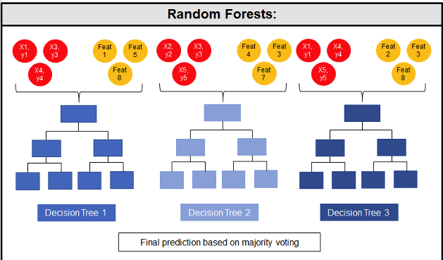
Random Forest models can be used for classification and regression types of problems, which form the majority of machine learning systems and solutions. For classification problems, this is where the target variable has either a binary value or a small number of defined values. For classification problems the Random Forest model will evaluate the predicted value for each of the decision trees in the model. The final predicted outcome will be the majority vote for all the decision trees. For regression problems the predicted value is numeric and on some range or scale. For example, we might want to predict a customer’s lifetime value (LTV), or the potential value of an insurance claim, etc. With Random Forest, each decision tree will make a prediction of this numeric value. The algorithm will then average these values for the final predicted outcome.
Under the hood, Random Forest is a collection of decision trees. Although decision trees are a popular algorithm for machine learning, they can have a tendency to over fit the model. This can lead higher than expected errors when predicting unseen data. It also gives just one possible way of representing the data and being able to derive a possible predicted outcome.
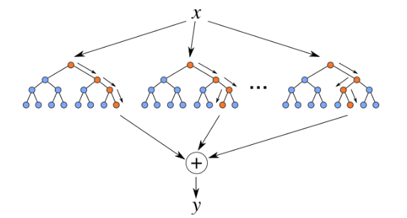 Random Forest on the other hand relies of the predicted outcomes from many different decision trees, each of which is built in a slightly different way. It is an ensemble technique that combines the predicted outcomes from each decision tree to give one answer. Typically, the number of trees created by the Random Forest algorithm is defined by a parameter setting, and in most languages this can default to 100+ or 200+ trees.
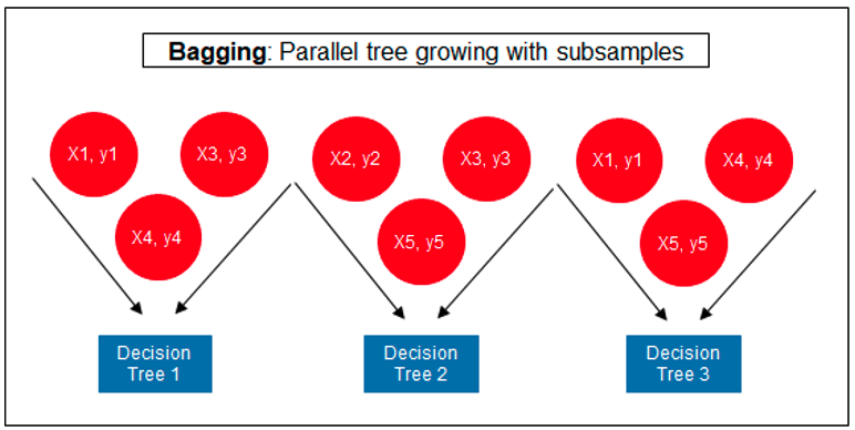
The Random Forest algorithm has three main features:
- It uses a method called bagging to create different subsets of the original training data
- It will randomly section different subsets of the features/attributes and build the decision tree based on this subset
- By creating many different decision trees, based on different subsets of the training data and different subsets of the features, it will increase the probability of capturing all possible ways of modeling the data
For each decision tree produced, the algorithm will use a measure, such as the Gini Index, to select the attributes to split on at each node of the decision tree.
To create a RandomForest model using Oracle Data Mining, you will follow the same process as with any of the other algorithms, the core of these are:
- define the parameter settings
- create the model
- score/label new data
Let’s start with the first step, defining the parameters. As with all the classification algorithms the same or similar parameters are set. With RandomForest we can set an additional parameter which tells the algorithm how many decision trees to create as part of the model. By default, 20 decision trees will be created. But if you want to change this number you can use the RFOR_NUM_TREES parameter. Remember the larger the value the longer it will take to create the model. But will have better accuracy. On the other hand with a small number of trees the quicker the model build will be, but might night be as accurate. This is something you will need to explore and determine. In the following example I change the number of trees to created to ten.
CREATE TABLE BANKING_RF_SETTINGS (
    SETTING_NAME VARCHAR2(50),
    SETTING_VALUE VARCHAR2(50)
);

BEGIN
  DELETE FROM BANKING_RF_SETTINGS;

  INSERT INTO banking_RF_settings (setting_name, setting_value)
  VALUES (dbms_data_mining.algo_name, dbms_data_mining.algo_random_forest);

  INSERT INTO banking_RF_settings (setting_name, setting_value)
  VALUES (dbms_data_mining.prep_auto, dbms_data_mining.prep_auto_on);

  INSERT INTO banking_RF_settings (setting_name, setting_value)
  VALUES (dbms_data_mining.RFOR_NUM_TREES, 10);

  COMMIT;
END;
Other default parameters used include, for creating each decision tree, use random 50% selection of columns and 50% sample of training data.
Now for step 2, create the model.
DECLARE
   v_start_time  TIMESTAMP;
BEGIN
   DBMS_DATA_MINING.DROP_MODEL('BANKING_RF_72K_1');

   v_start_time := current_timestamp;

   DBMS_DATA_MINING.CREATE_MODEL(
      model_name          => 'BANKING_RF_72K_1',
      mining_function     => dbms_data_mining.classification,
      data_table_name     => 'BANKING_72K',
      case_id_column_name => 'ID',
      target_column_name  => 'TARGET',
      settings_table_name => 'BANKING_RF_SETTINGS');

   dbms_output.put_line('Time take to create model = ' || to_char(extract(second from (current_timestamp-v_start_time))) || ' seconds.');
END;
The above code measures how long it takes to create the model.
I’ve run this same parameters and create models for different training data set sizes. I’ve also changed the number of decision trees to create. The following table shows the timings.
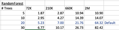
You can see it took 5.23 seconds to create a RandomForest model using the default settings for a data set of 72K records. This increase to just over one minute for a data set of 2 million records. Yo can also see the effect of reducing the number of decision trees on how long it takes the create model to run.
For step 3, on using the model on new data, this is just the same as with any of the classification models. Here is an example:
SELECT cust_id, target,
       prediction(BANKING_RF_72K_1 USING *)  predicted_value,
       prediction_probability(BANKING_RF_72K_1 USING *) probability
FROM   bank_test_v;
That’s it. That’s all there is to creating a RandomForest machine learning model using Oracle Machine Learning.
It’s quick and easy 🙂
GoLang – Consuming Oracle REST API from an Oracle Cloud Database)
Does anyone write code to access data in a database anymore, and by code I mean SQL? The answer to this question is ‘It Depends’, just like everything in IT.
Using REST APIs is very common for accessing processing data with a Database. From using an API to retrieve data, to using a slightly different API to insert data, and using other typical REST functions to perform your typical CRUD operations. Using REST APIs allows developers to focus on write efficient applications in a particular application, instead of having to swap between their programming language and SQL. In later cases most developers are not expert SQL developer or know how to work efficiently with the data. Therefore leave the SQL and procedural coding to those who are good at that, and then expose the data and their code via REST APIs. The end result is efficient SQL and Database coding, and efficient application coding. This is a win-win for everyone.
I’ve written before about creating REST APIs in an Oracle Cloud Database (DBaaS and Autonomous). In these writings I’ve shown how to use the in-database machine learning features and to use REST APIs to create an interface to the Machine Learning models. These models can be used to to score new data, making a machine learning prediction. The data being used for the prediction doesn’t have to exist in the database, instead the database is being used as a machine learning scoring engine, accessed using a REST API.
In that article I showed how easy it was to use the in-database machine model using Python.
Python has a huge fan and user base, but some of the challenges with Python is with performance, as it is an interrupted language. Don’t get be wrong on this, as lots of work has gone into making Python more efficient. But in some scenarios it just isn’t fast enough. In does scenarios people will switch into using other quicker to execute languages such as C, C++, Java and GoLang.
Here is the GoLang code to call the in-database machine learning model and process the returned data.
import (
    "bytes"
    "encoding/json"
    "fmt"
    "io/ioutil"
    "net/http"
    "os"
)

func main() {
    fmt.Println("---------------------------------------------------")
    fmt.Println("Starting Demo - Calling Oracle in-database ML Model")
    fmt.Println("")

    // Define variables for REST API and parameter for first prediction
    rest_api = "<full REST API>"

    // This wine is Bad
    a_country := "Portugal"
    a_province := "Douro"
    a_variety := "Portuguese Red"
    a_price := "30"

    // call the REST API adding in the parameters
    response, err := http.Get(rest_api +"/"+ a_country +"/"+ a_province +"/"+ a_variety +"/"+ a_price)
    if err != nil {
        // an error has occurred. Exit
        fmt.Printf("The HTTP request failed with error :: %s\n", err)
        os.Exit(1)
    } else {
        // we got data! Now extract it and print to screen
        responseData, _ := ioutil.ReadAll(response.Body)
        fmt.Println(string(responseData))
    }
    response.Body.Close()

    // Lets do call it again with a different set of parameters

    // This wine is Good - same details except the price is different
    a_price := "31"

    // call the REST API adding in the parameters
    response, err := http.Get(rest_api +"/"+ a_country +"/"+ a_province +"/"+ a_variety +"/"+ a_price)
    if err != nil {
        // an error has occurred. Exit
        fmt.Printf("The HTTP request failed with error :: %s\n", err)
        os.Exit(1)
    } else {
        responseData, _ := ioutil.ReadAll(response.Body)
        fmt.Println(string(responseData))
    }
    defer response.Body.Close()

    // All done!
    fmt.Println("")
    fmt.Println("...Finished Demo ...")
    fmt.Println("---------------------------------------------------")
}
XGBoost in Oracle 20c
 Updated: Changed 20c to Oracle 21c, as Oracle 20c Database never really existed 🙂
Another of the new machine learning algorithms in Oracle 21c Database is called XGBoost. Most people will have come across this algorithm due to its recent popularity with winners of Kaggle competitions and other similar events.
XGBoost is an open source software library providing a gradient boosting framework in most of the commonly used data science, machine learning and software development languages. It has it’s origins back in 2014, but the first official academic publication on the algorithm was published in 2016 by Tianqi Chen and Carlos Guestrin, from the University of Washington.
The algorithm builds upon the previous work on Decision Trees, Bagging, Random Forest, Boosting and Gradient Boosting. The benefits of using these various approaches are well know, researched, developed and proven over many years. XGBoost can be used for the typical use cases of Classification including classification, regression and ranking problems. Check out the original research paper for more details of the inner workings of the algorithm.
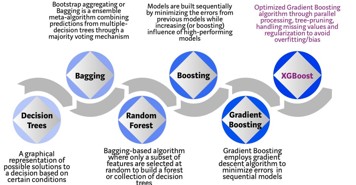
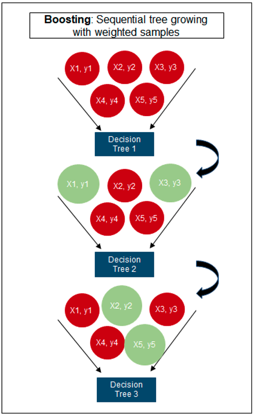
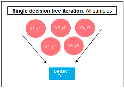
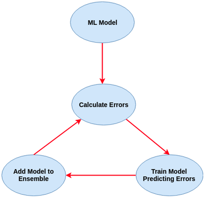 Regular machine learning models, like Decision Trees, simply train a single model using a training data set, and only this model is used for predictions. Although a Decision Tree is very simple to create (and very very quick to do so) its predictive power may not be as good as most other algorithms, despite providing model explainability. To overcome this limitation ensemble approaches can be used to create multiple Decision Trees and combines these for predictive purposes. Bagging is an approach where the predictions from multiple DT models are combined using majority voting. Building upon the bagging approach Random Forest uses different subsets of features and subsets of the training data, combining these in different ways to create a collection of DT models and presented as one model to the user. Boosting takes a more iterative approach to refining the models by building sequential models with each subsequent model is focused on minimizing the errors of the previous model. Gradient Boosting uses gradient descent algorithm to minimize errors in subsequent models. Finally with XGBoost builds upon these previous steps enabling parallel processing, tree pruning, missing data treatment, regularization and better cache, memory and hardware optimization. It’s commonly referred to as gradient boosting on steroids.
The following three images illustrates the differences between Decision Trees, Random Forest and XGBoost.
The XGBoost algorithm in Oracle 20c has over 40 different parameter settings, and with most scenarios the default settings with be fine for most scenarios. Only after creating a baseline model with the details will you look to explore making changes to these. Some of the typical settings include:
- Booster = gbtree
- #rounds for boosting = 10
- max_depth = 6
- num_parallel_tree = 1
- eval_metric = Classification error rate or RMSE for regression
As with most of the Oracle in-database machine learning algorithms, the setup and defining the parameters is really simple. Here is an example of minimum of parameter settings that needs to be defined.
BEGIN
   -- delete previous setttings
   DELETE FROM banking_xgb_settings;

   INSERT INTO BANKING_XGB_SETTINGS (setting_name, setting_value)
   VALUES (dbms_data_mining.algo_name, dbms_data_mining.algo_xgboost);

   -- For 0/1 target, choose binary:logistic as the objective.
   INSERT INTO BANKING_XGB_SETTINGS (setting_name, setting_value)
   VALUES (dbms_data_mining.xgboost_objective, 'binary:logistic’);

   commit;
END;
To create an XGBoost model run the following.


BEGIN
   DBMS_DATA_MINING.CREATE_MODEL (
      model_name          => 'BANKING_XGB_MODEL',
      mining_function     => dbms_data_mining.classification,
      data_table_name     => 'BANKING_72K',
      case_id_column_name => 'ID',
      target_column_name  => 'TARGET',
      settings_table_name => 'BANKING_XGB_SETTINGS');
END;
That’s all nice and simple, as it should be, and the new model can be called in the same manner as any of the other in-database machine learning models using functions like PREDICTION, PREDICTION_PROBABILITY, etc.
One of the interesting things I found when experimenting with XGBoost was the time it took to create the completed model. Using the default settings the following table gives the time taken, in seconds to create the model.
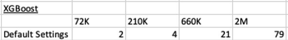
As you can see it is VERY quick even for large data sets and gives greater predictive accuracy.
- ← Previous
- 1
- 2
- 3
- 4
- Next →

You must be logged in to post a comment.