
oracle cloud
Oracle Object Storage – Setup and Explore
This blog post will walk you through how to access Oracle OCI Object Storage and explore what buckets and files you have there, using Python and the OCI Python library. There will be additional posts which will walk through some of the other typical tasks you’ll need to perform with moving files into and out of OCI Object Storage.
- Oracle Object Storage – Buckets & Loading files
- Oracle Object Storage – Downloading and Deleting
- Oracle Object Storage – Parallel Uploading
The first thing you’ll need to do is to install the OCI Python library. You can do this by running pip command or if using Anaconda using their GUI for doing this. For example,
pip3 install ociCheck out the OCI Python documentation for more details.
Next, you’ll need to get and setup the configuration settings and download the pem file.
We need to create the config file that will contain the required credentials and information for working with OCI. By default, this file is stored in : ~/.oci/config
mkdir ~/oci
cd oci
Now create the config file, using vi or something similar.
vi config
Edit the file to contain the following, but look out for the parts that need to be changed/updated to match your OCI account details.
[ADMIN_USER]user=ocid1.user.oc1..<unique_ID>
fingerprint=<your_fingerprint>
tenancy = ocid1.tenancy.oc1..<unique_ID>
region = us-phoenix-1key_file=
<path to key .pem file>
The above details can be generated by creating an API key for your OCI user. Copy and paste the default details to the config file.
- [ADMIN_USER] > you can name this anything you want, but it will referenced in Python.
- user > enter the user ocid. OCID is the unique resource identifier that OCI provides for each resource.
- fingerprint > refers to the fingerprint of the public key you configured for the user.
- tenancy > your tenancy OCID.
- region > the region that you are subscribed to.
- key_file > the path to the .pem file you generated.

Just download the .pem file and the config file details. Add them to the config file, and give the full path to the .epm file, including its name.
You are now ready to use the OCI Python library to access and use your OCI cloud environment. Let’s run some tests to see if everything works and connects ok.
#import libraries
import oci
import json
import os
import io

#load the config file
config = oci.config.from_file("~/.oci/config")
config

#only part of the output is displayed due to security reasons
{'log_requests': False, 'additional_user_agent': '', 'pass_phrase': None, 'user': 'oci...........
We can now define some core variables.
#My Compartment ID
COMPARTMENT_ID = "ocid1.tenancy.oc1..............

#Object storage Namespace
object_storage_client = oci.object_storage.ObjectStorageClient(config)
NAMESPACE = object_storage_client.get_namespace().data

#Name of Bucket for this demo
BUCKET_NAME = 'DEMO_Bucket'
We can now define some functions to:
- List the Buckets in my OCI account
- List the number of files in each Bucket
- Number of files in a particular Bucket
- Check for Bucket Existence
def list_buckets():
    l_buckets = object_storage_client.list_buckets(NAMESPACE, COMPARTMENT_ID).data
    # Get the data from response
    for bucket in l_buckets:
        print(bucket.name)

def list_bucket_counts():
    l_buckets = object_storage_client.list_buckets(NAMESPACE, COMPARTMENT_ID).data
    for bucket in l_buckets:
        print("Bucket name: ",bucket.name)
        buck_name = bucket.name
        objects = object_storage_client.list_objects(NAMESPACE, buck_name).data
        count = 0
        for i in objects.objects:
            count+=1

        print('... num of objects :', count)

def check_bucket_exists(b_name):
    #check if Bucket exists
    is_there = False
    l_b = object_storage_client.list_buckets(NAMESPACE, COMPARTMENT_ID).data
    for bucket in l_b:
        if bucket.name == b_name:
            is_there = True

    if is_there == True:
        print(f'Bucket {b_name} exists.')
    else:
        print(f'Bucket {b_name} does not exist.')

    return is_there

def list_bucket_details(b):
    bucket_exists = check_bucket_exists(b)
    if bucket_exists == True:
        objects = object_storage_client.list_objects(NAMESPACE, b).data
        count = 0
        for i in objects.objects:
            count+=1

        print(f'Bucket {b} has objects :', count)
Now we can run these functions to test them. Before running these make sure you can create a connection to OCI.

Python for OCI installation and configuration
Having set up your Oracle Cloud account and perhaps initiated some services, such as an Autonomous Database or an AI Service, you have some options with how you’ll interact with those services. The first is to use the online interfaces and tools for them. Another is to access these OCI services from your local PC or laptop. This latter method gives you greater flexibility for accessing these services, automating various tasks and building out some applications. This post will step through how to install the necessary Python library, how to configure for connecting to OCI and will demo some of the simpler APIs for accessing the OCI services. This will help you verify your connection is working correctly.
The simple part of this is installing the OCI library!
pip3 install oci
Like I said that’s the simple part.
The next step involves the configuration of a connection to your OCI tenancy. But before you can do this you need to have an account on OCI. If you don’t have one already, the easiest and FREE way to do this is to set up an account on the Oracle Free Tier. There is some Free stuff you can use, plus getting a few hundred dollars to spend on some of the other non-Free cloud services. When you’ve completed this you can move on to the next step.
We need to create the config file that will contain the required credentials and information for working with OCI. By default, this file is stored in : ~/.oci/config
mkdir ~/oci
cd oci
Now create the config file, using vi or something similar.
vi config
Edit the file to contain the following, but look out for the parts that need to be changed/updated to match your OCI account details.
[ADMIN_USER]
user=ocid1.user.oc1..<unique_ID>
fingerprint=<your_fingerprint>
tenancy = ocid1.tenancy.oc1..<unique_ID>
region = us-phoenix-1
key_file=<path to key .pem file>
The above details can be generated by creating an API key for your OCI user. Copy and Pate the default details to the config file.
- [ADMIN_USER] > you can name this anything you want, but it will referenced in Python.
- user > enter the user ocid. OCID is the unique resource identifier that OCI provides for each resource.
- fingerprint > refers to the fingerprint of the public key you configured for the user.
- tenancy > your tenancy OCID.
- region > the region that you are subscribed to.
- key_file > the path to the .pem file you generated.
Just download the .epm file and the config file details. Add them to the config file, and give the full path to the .epm file, including it’s name.
You are now ready to use the OCI Python library to access and use your OCI cloud environment. Let’s run some tests to see if everything works and connects ok.
config = oci.config.from_file(
     "~/.oci/config")
identity = oci.identity.IdentityClient(config)
user = identity.get_user(config["user"]).data
print(user)
The above connects to OCI using the config file we’ve just created and will print the following details about the connect.

The following lists all the available shapes available to me in the us-ashburn-1 region.
database_client = oci.database.DatabaseClient(config)

# Send the request to service, some parameters are not required, see API
# doc for more info
list_db_system_shapes_response = database_client.list_db_system_shapes(
    compartment_id=compart_id,
    availability_domain="us-ashburn-1")

# Get the data from response
print(list_db_system_shapes_response.data)
The listing for the above is very long, so I’ll leave that for you to explore.
For more details of the APIs available check out the Documentation and the GitHub Respository for more examples.
OCI Data Labeling for Machine Learning
OCI Data Labeling is a service that enables developers and data scientists to construct labelled datasets for training AI and machine learning models. By utilizing OCI Data Labeling, users can easily gather data, generate datasets, and assign labels to individual data records through user-friendly interfaces and public APIs. The labelled datasets can then be utilised to facilitate model development across a wide range of Oracle’s AI and data science services, ensuring a seamless and efficient model-building experience.
OCI Data Labeling allows developers and data scientists to label different types of data for training AI and machine learning models. Here are some examples of how OCI Data Labeling can be used for different types of data:
- Document Labeling
- Image Labeling
- Text Labeling
Typically the labelling of data is a manual task but there are also options to programmicly do this if the necessary label data is available.

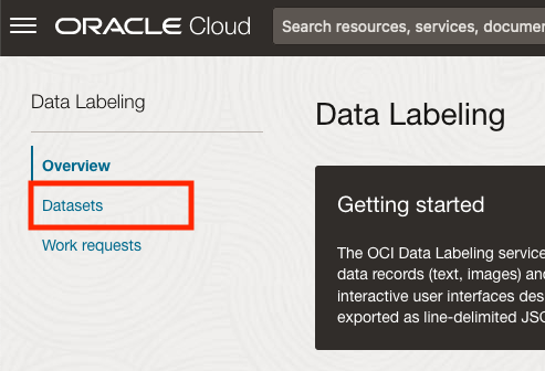
The OCI Data Labeling service can be located under the Analytics & AI menu. See the image.
As we want to label a dataset, we need to first define the Dataset we want to use.
Select Datasets from the menu.
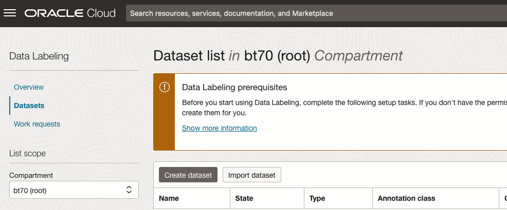
There are two options for creating the data set for labeling. The first is to use the Create Dataset option and the second is to Import Dataset.
If you already have your data in a Bucket, you can use both approaches. If you have a new dataset to import then use the Create Dataset option.
In this post, I’ll use the Create Dataset option and step through it.
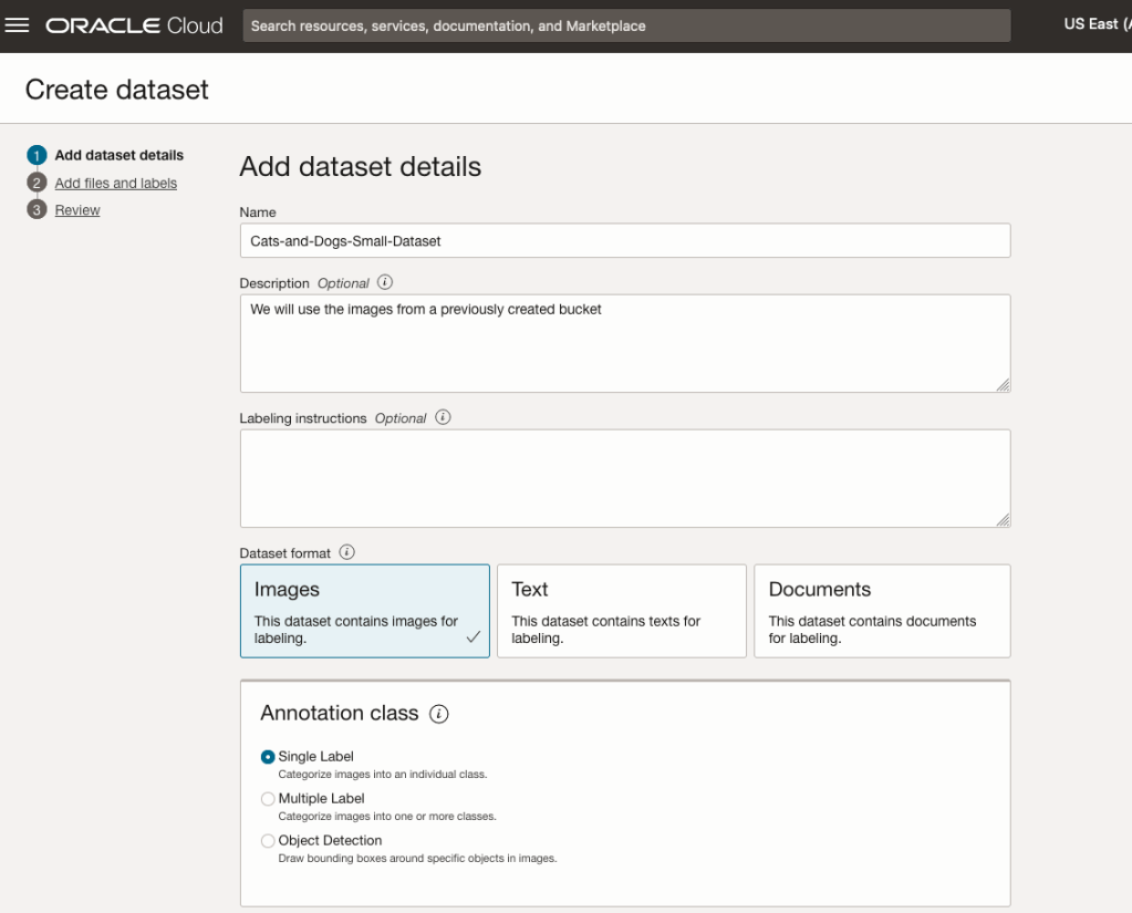
Start by giving a name to the Dataset, then specify the type of data (Images, Text or Documents). In this example, we will work with image data.
Then select if the dataset (or each image) has one or multiple labels, or if you are going to draw bounding boxes for Object Detection.
For our example, select Single Label.
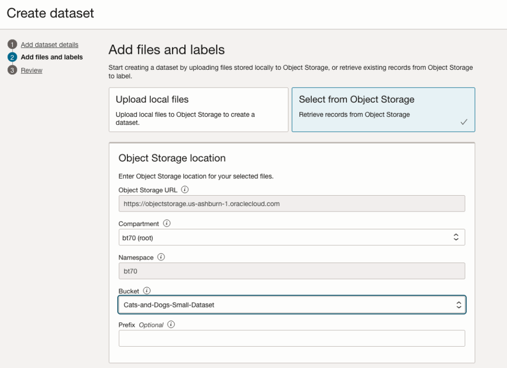
You can upload files from your computer or use files in an Object Bucket. As the dataset has already been loaded into a Bucket, we’ll select that option.
The Object Storage URL, Compartment and Namespace will be automatically populated for you.
Select the Bucket you want to use from the drop-down list. This dataset has 50 images each of Cats and Dogs.
The page will display the first eight or so, of the images in the Bucket. You can scroll through the others and this gives you a visual opportunity to make sure you are using the correct dataset.
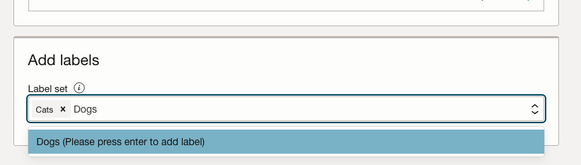
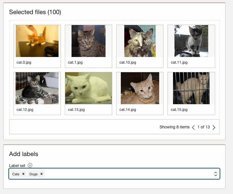
Now you can define the Labels to use for the dataset. In our sample dataset we only have two possible labels. If your dataset has more than this just enter the name and present enter. The Lable will be created.
You can add and remove labels.
When finished click the Next button at the bottom of the screen.
The final part of this initial setup is to create the dataset by clicking on the Create button
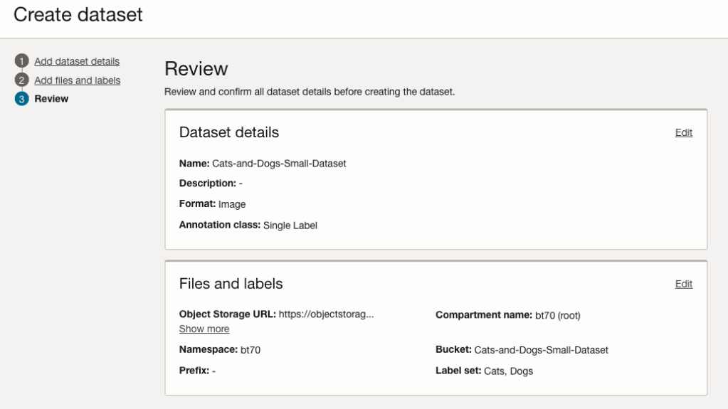
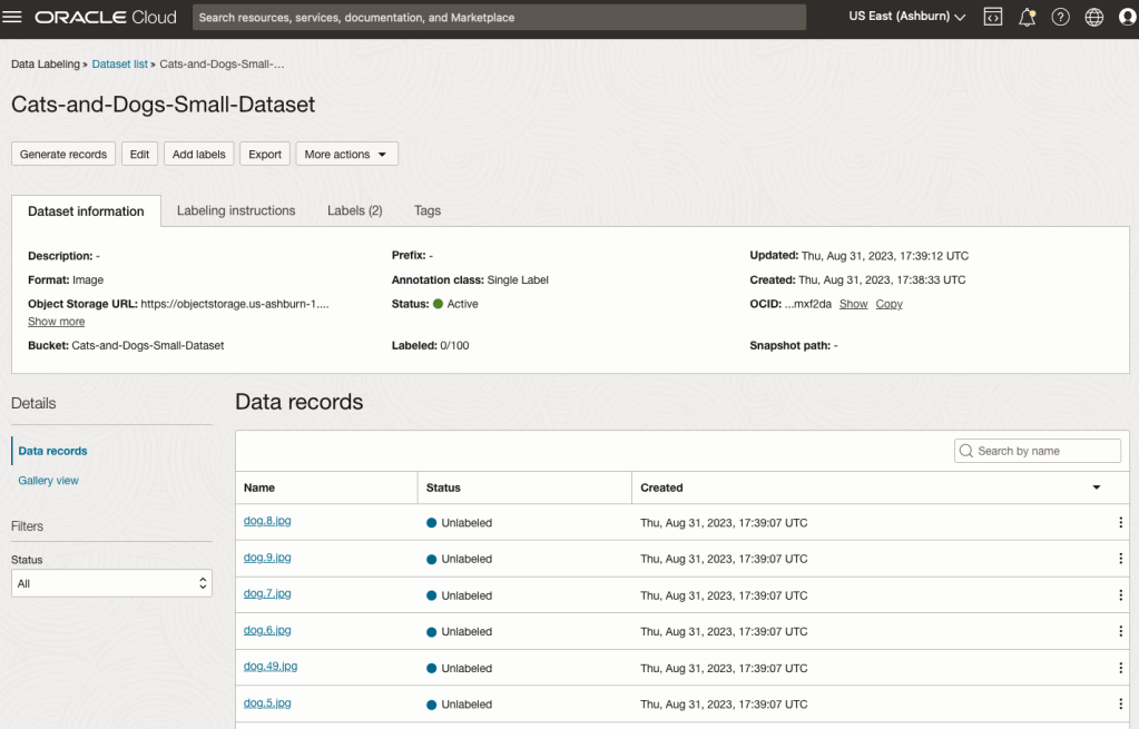
When everything has been processed you will get a screen that looks like this.
You are now ready to move on to labelling the dataset.
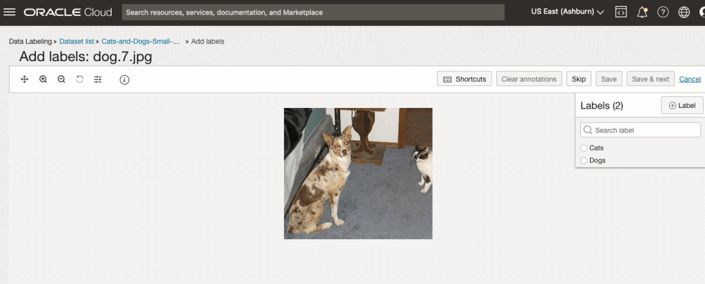
To label each image, start by clicking on the first image. This will open a screen like what is shown (to the right).
Click on the radio group item for the label that best represents the image. In some scenarios maybe both labels are suitable, and in such cases just pick the most suitable one. In this example, I’ve selected Dog. An alternative approach is to use the bounding box labelling. I’ll have a different post illustrating that.
Select the most suitable label and then click ‘Save & next’ button.
Yes, you’ll need to do this for all the images in the dataset. Yes, this can take a lot of time, particularly if you have 100s, or 1000s of images. The Datasets screen has details of how many images have been labelled and or not, and you can easily search for unlabelled files and continue labelling, if you need to take a break.
OCI Object Storage Buckets
We can upload and store data in Object Storage on OCI. This allows us to load and store data in a variety of different formats and sizes. With this data/files in object storage, it can be easily accessed from an Oracle Database (e.g. Autonomous Database) and any other service on OCI. This allows building more complete business solutions in a more integrated way.
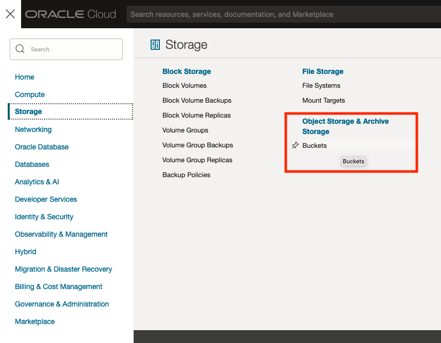
The Buckets feature can be found under the Storage option in the main Menu. From the popup screen look under Object Storage & Archive Storage and click on Buckets.
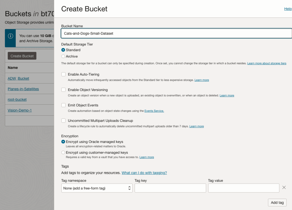
In the Objects Storage screen click on Create Bucket button.
In the Create Bucket screen, change the name of the Bucket. In this example, I’ve called it ‘Cats-and-Dogs-Small-Dataset’. No spaces are allowed. You can leave the defaults for the other settings. Then click the Create button.
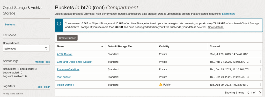
It will then be displayed along with any other buckets you have. I’ve a few other buckets.
Click on the Bucket name to open the bucket and add files to it.
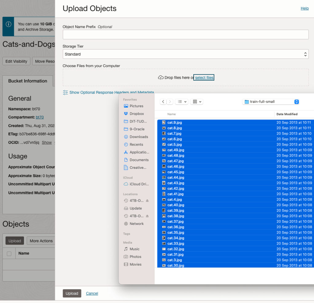
Click on the Upload button. Locate the files on your computer, select the files you want to upload.
The files will be listed in the Upload Object window. Click the Upload button to start transferring them to OCI.
If you wish you can set a prefix for all the files being uploaded.
When the files have been uploaded, click the Close button.
Note: The larger the dateset, in files and file size, it can take some time (depending on interest connection speed) for all the files to load into the Bucket.
To view the details of an image, click on the three dots to the right of the image files. This will open a menu for the image, where you can select to view image Details, download, copy, rename, delete, etc. the image.
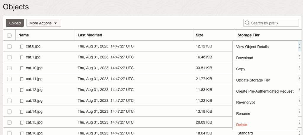

Click on View Object Details to get the details of the image.
This will display details about the object and the URI for the image.
Machine Learning App Migration to Oracle Cloud VM
Over the past few years, I’ve been developing a Stock Market prediction algorithm and made some critical refinements to it earlier this year. As with all analytics, data science, machine learning and AI projects, testing is vital to ensure its performance, accuracy and sustainability. Taking such a project out of a lab environment and putting it into a production setting introduces all sorts of different challenges. Some of these challenges include being able to self-manage its own process, logging, traceability, error and event management, etc. Automation is key and implementing all of these extra requirements tasks way more code and time than developing the actual algorithm. Typically, the machine learning and algorithms code only accounts for less than five percent of the actual code, and in some cases, it can be less than one percent!
I’ve come to the stage of deploying my App to a production-type environment, as I’ve been running it from my laptop and then a desktop for over a year now. It’s now 100% self-managing so it’s time to deploy. The environment I’ve chosen is using one of the Virtual Machines (VM) available on the Oracle Free Tier. This means it won’t cost me a cent (dollar or more) to run my App 24×7.
My App has three different components which use a core underlying machine learning predictions engine. Each is focused on a different set of stock markets. These marks operate in the different timezone of US markets, European Markets and Asian Markets. Each will run on a slightly different schedule than the rest.
The steps outlined below take you through what I had to do to get my App up and running the VM (Oracle Free Tier). It took about 20 minutes to complete everything
The first thing you need to do is create a ssh key file. There are a number of ways of doing this and the following is an example.
ssh-keygen -t rsa -N "" -b 2048 -C "myOracleCloudkey" -f myOracleCloudkey
This key file will be used during the creation of the VM and for logging into the VM.
Log into your Oracle Cloud account and you’ll find the Create Instances Compute i.e. create a virtual machine/

Complete the Create Instance form and upload the ssh file you created earlier. Then click the Create button. This assumes you have networking already created.

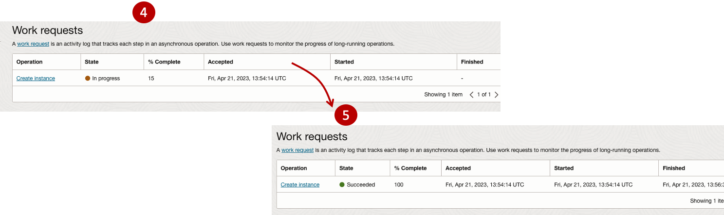
It will take a minute or two for the VM to be created and you can monitor the progress.
After it has been created you need to click on the start button to start the VM.
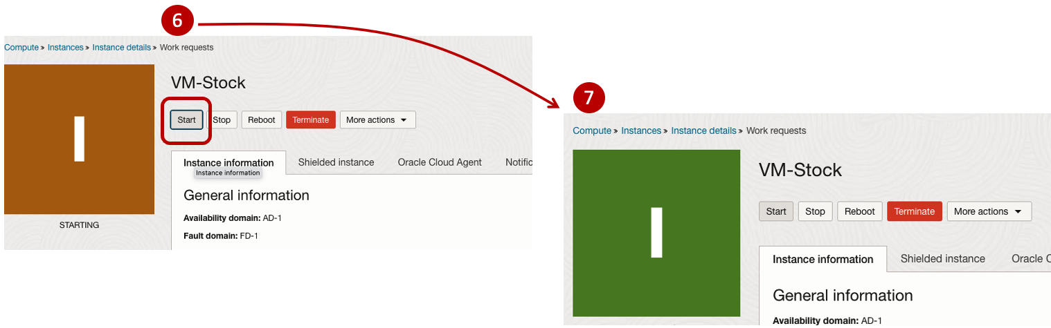
After it has started you can now log into the VM from a terminal window, using the public IP address
ssh -i myOracleCloudKey opc@xxx.xxx.xxx.xxxAfter you’ve logged into the VM it’s a good idea to run an update.
[opc@vm-stocks ~]$ sudo yum -y update
Last metadata expiration check: 0:13:53 ago on Fri 21 Apr 2023 14:39:59 GMT.
Dependencies resolved.
========================================================================================================================
 Package                         Arch       Version                                          Repository            Size
========================================================================================================================
Installing:
 kernel-uek                      aarch64    5.15.0-100.96.32.el8uek                          ol8_UEKR7            1.4 M
 kernel-uek-core                 aarch64    5.15.0-100.96.32.el8uek                          ol8_UEKR7             47 M
 kernel-uek-devel                aarch64    5.15.0-100.96.32.el8uek                          ol8_UEKR7             19 M
 kernel-uek-modules              aarch64    5.15.0-100.96.32.el8uek                          ol8_UEKR7             59 M
Upgrading:
 NetworkManager                  aarch64    1:1.40.0-6.0.1.el8_7                             ol8_baseos_latest    2.1 M
 NetworkManager-config-server    noarch     1:1.40.0-6.0.1.el8_7                             ol8_baseos_latest    141 k
 NetworkManager-libnm            aarch64    1:1.40.0-6.0.1.el8_7                             ol8_baseos_latest    1.9 M
 NetworkManager-team             aarch64    1:1.40.0-6.0.1.el8_7                             ol8_baseos_latest    156 k
 NetworkManager-tui              aarch64    1:1.40.0-6.0.1.el8_7                             ol8_baseos_latest    339 k
...
...
The VM is now ready to setup and install my App. The first step is to install Python, as all my code is written in Python.
[opc@vm-stocks ~]$ sudo yum install -y python39
Last metadata expiration check: 0:20:35 ago on Fri 21 Apr 2023 14:39:59 GMT.
Dependencies resolved.
========================================================================================================================
 Package                         Architecture  Version                                        Repository           Size
========================================================================================================================
Installing:
 python39                        aarch64       3.9.13-2.module+el8.7.0+20879+a85b87b0         ol8_appstream        33 k
Installing dependencies:
 python39-libs                   aarch64       3.9.13-2.module+el8.7.0+20879+a85b87b0         ol8_appstream       8.1 M
 python39-pip-wheel              noarch        20.2.4-7.module+el8.6.0+20625+ee813db2         ol8_appstream       1.1 M
 python39-setuptools-wheel       noarch        50.3.2-4.module+el8.5.0+20364+c7fe1181         ol8_appstream       497 k
Installing weak dependencies:
 python39-pip                    noarch        20.2.4-7.module+el8.6.0+20625+ee813db2         ol8_appstream       1.9 M
 python39-setuptools             noarch        50.3.2-4.module+el8.5.0+20364+c7fe1181         ol8_appstream       871 k
Enabling module streams:
 python39                                      3.9

Transaction Summary
========================================================================================================================
Install  6 Packages

Total download size: 12 M
Installed size: 47 M
Downloading Packages:
(1/6): python39-pip-20.2.4-7.module+el8.6.0+20625+ee813db2.noarch.rpm                    23 MB/s | 1.9 MB     00:00
(2/6): python39-pip-wheel-20.2.4-7.module+el8.6.0+20625+ee813db2.noarch.rpm             5.5 MB/s | 1.1 MB     00:00
...
...
Next copy the code to the VM, setup the environment variables and create any necessary directories required for logging. The final part of this is to download the connection Wallett for the Database. I’m using the Python library oracledb, as this requires no additional setup.
Then install all the necessary Python libraries used in the code, for example, pandas, matplotlib, tabulate, seaborn, telegram, etc (this is just a subset of what I needed). For example here is the command to install pandas.
pip3.9 install pandasAfter all of that, it’s time to test the setup to make sure everything runs correctly.
The final step is to schedule the App/Code to run. Before setting the schedule just do a quick test to see what timezone the VM is running with. Run the date command and you can see what it is. In my case, the VM is running GMT which based on the current time locally, the VM was showing to be one hour off. Allowing for this adjustment and for day-light saving time, the time +/- markets openings can be set. The following example illustrates setting up crontab to run the App, Monday-Friday, between 13:00-22:00 and at 5-minute intervals. Open crontab and edit the schedule and command. The following is an example
> contab -e

*/5 13-22 * * 1-5 python3.9 /home/opc/Stocks.py >Stocks.txt
For some stock market trading apps, you might want it to run more frequently (than every 5 minutes) or less frequently depending on your strategy.
After scheduling the components for each of the Geographic Stock Market areas, the instant messaging of trades started to appear within a couple of minutes. After a little monitoring and validation checking, it was clear everything was running as expected. It was time to sit back and relax and see how this adventure unfolds.
For anyone interested, the App does automated trading with different brokers across the markets, while logging all events and trades to an Oracle Autonomous Database (Free Tier = no cost), and sends instant messages to me notifying me of the automated trades. All I have to do is Nothing, yes Nothing, only to monitor the trade notifications. I mentioned earlier the importance of testing, and with back-testing of the recent changes/improvements (as of the date of post), the App has given a minimum of 84% annual return each year for the past 15 years. Most years the return has been a lot more!
How many Data Center Regions by Vendor?
There has been some discussions over the past weeks, months, years on which Cloud provider is the best, or the biggest, or provides the most services, or [insert some other topic]? The old answer to everything related to IT is ‘It Depends’. A recent article by CloudWars (and updated numbers by them) and some of the comments to it, and elsewhere prompted me to have a look at ‘How Many Data Center Regions do each Cloud Vendor have?’ I didn’t go looking at all possible cloud vendors, but instead kept to the main vendors consisting of Microsoft Azure, Google Cloud Platform (GCP), Oracle Cloud and Amazon Web Services (AWS). We know AWS has been around for a long long time, and seems to gather most of the attention and focus within the developer community, etc, you’d expect them to be the biggest. Well, the results from my investigation does not support this.
Now, it is important to remember when reading the results presented below that these are from a particular point in time, and that is the date of this blog post. If you are reading this some time later, the actual number of data centers will be different and will be larger.
When looking at the data, as presented on each vendors website (see link to each vendor below), most list some locations coming in the future. It’s really impressive to see the number of “coming soon” locations. These “coming soon” locations are not included below (as of blog post date).
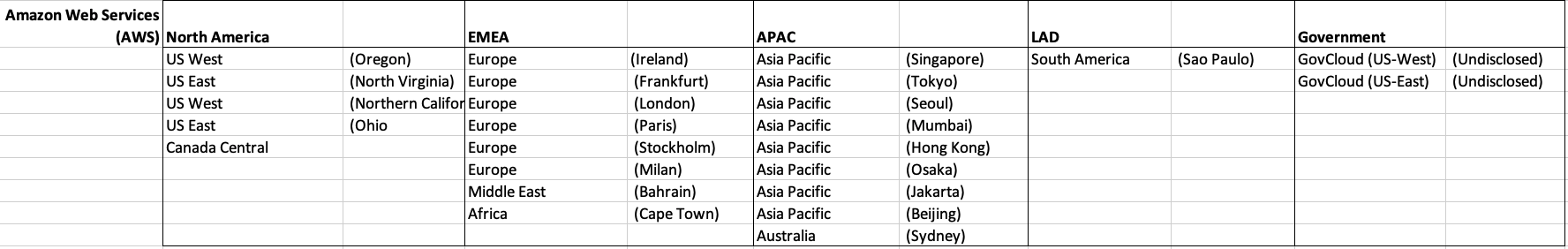
Before showing a breakdown for each vendor the following table gives the total number of data center regions for each vendor.
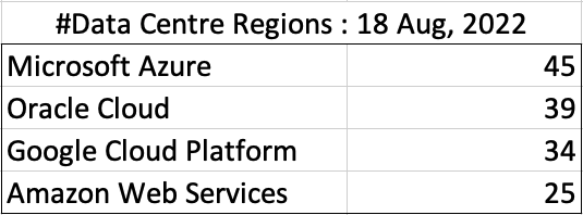
The numbers presented in the above table are different to does presented in the original CloudWars article or their updated numbers. If you look at the comments on that article and the comments on LinkedIn, you will see there was some disagreement of on their numbers. The problem is a data quality one, and vendors presenting their list of data centers in different parts of their website and documentation. Data quality and consistency is always a challenge, and particularly so when publishing data on vendor blogs, documentation and various websites. Indeed, the data I present in this post will be out of date within a few days/weeks. I’ve also excluded locations marked as ‘coming soon’ (see Azure listing).
Looking at the numbers in the above table can be a little surprising, particularly if you look at AWS, and then look at the difference in numbers between AWS and Azure and even Oracle. Very soon Azure will have double the number of data center regions when compared to AWS.
What do these numbers tell you? Based on just these numbers it would appear that Azure and Oracle Cloud are BIG cloud providers, and are much bigger than AWS. But maybe AWS has data centers that are way way bigger than those two vendors. It can be a little challenging to know the size and scale of each data center. Maybe they are going after different types of customers? With the roll out of Cloud over the past few years, there has been numerous challenges from legal and sovereign related issues requiring data to be geographically located within a country or geographic region. Most of these restrictions apply to larger organizations in the financial, insurance, and government related, etc. Given the historical customer base of Microsoft and Oracle, maybe this is driving their number of data center regions.
In more recent times there has been a growing interest, and in some sectors a growing need for organizations to be multi-cloud. Given the number of data center regions, for Azure and Oracle, and commonality in their geographic locations, it isn’t surprising to see the recent announcement from Azure and Oracle of their interconnect agreement and making the Oracle Database Service available (via interconnect) from Azure. I’m sure we will see more services being shared between these two vendors, and other might join in doing something similar.
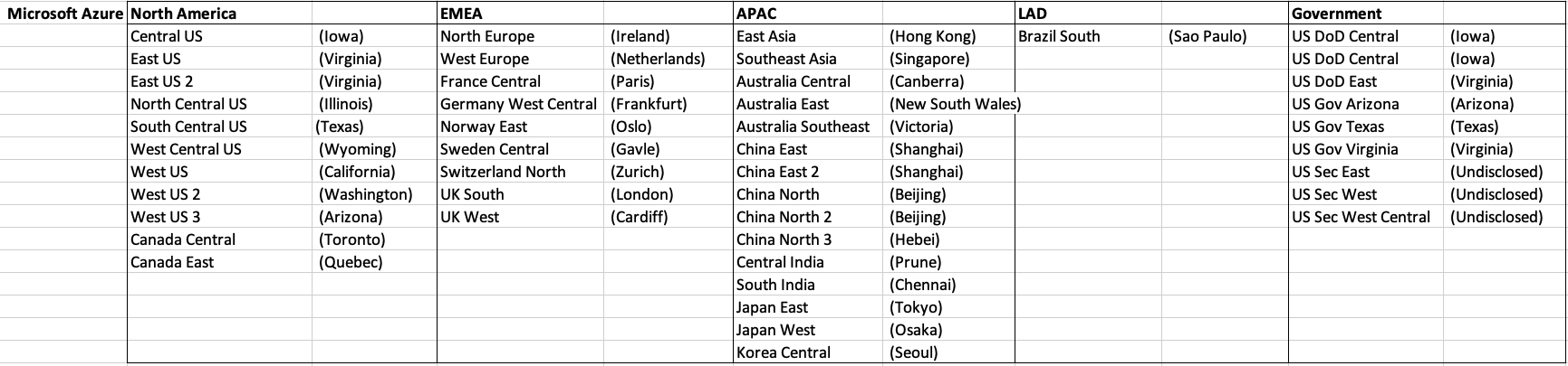
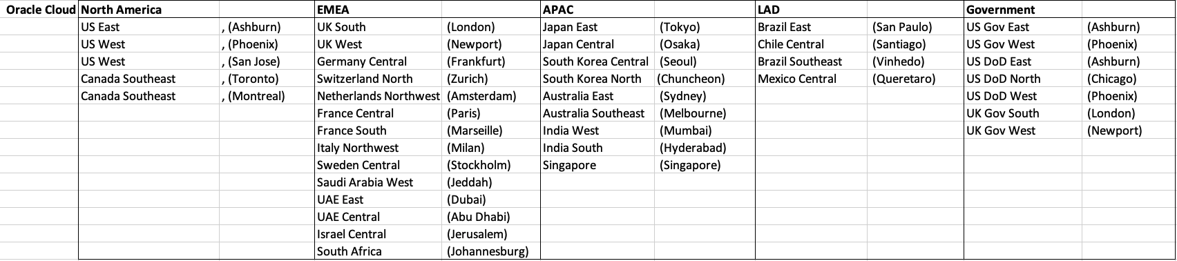
Let’s get back to the numbers and data for each Vendor. I’ve also included a link to the Vendor website where these data was obtained. (just remember these are based on date of blog post)
When you look at the Azure website listing the location, at first look it might appear they have many more locations. When you look closer at these, some/many of them are listed as ‘coming soon’. These ‘coming soon’ locations are not included in the above and below tables.
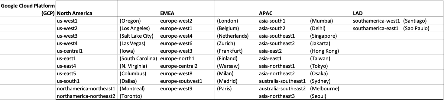
GCP doesn’t list and Government data center regions.
OCI Data Science – Create a Project & Notebook, and Explore the Interface
In my previous blog post I went through the steps of setting up OCI to allow you to access OCI Data Science. Those steps showed the setup and configuration for your Data Science Team.
In this post I will walk through the steps necessary to create an OCI Data Science Project and Notebook, and will then Explore the basic Notebook environment.
1 – Create a Project
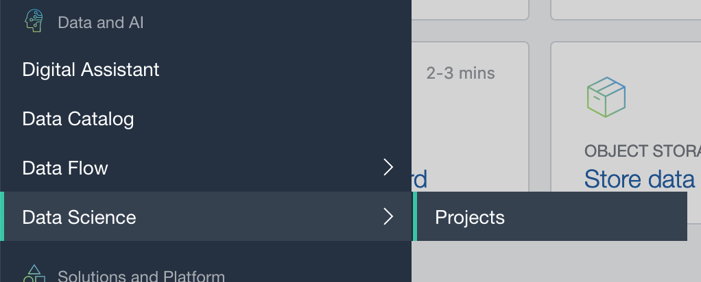
From the main menu on the Oracle Cloud home page select Data Science -> Projects from the menu.
Select the appropriate Compartment in the drop-down list on the left hand side of the screen. In my previous blog post I created a separate Compartment for my Data Science work and team. Then click on the Create Projects button.
 Enter a name for your project. I called this project, ‘DS-Demo-Project’. Click Create button.
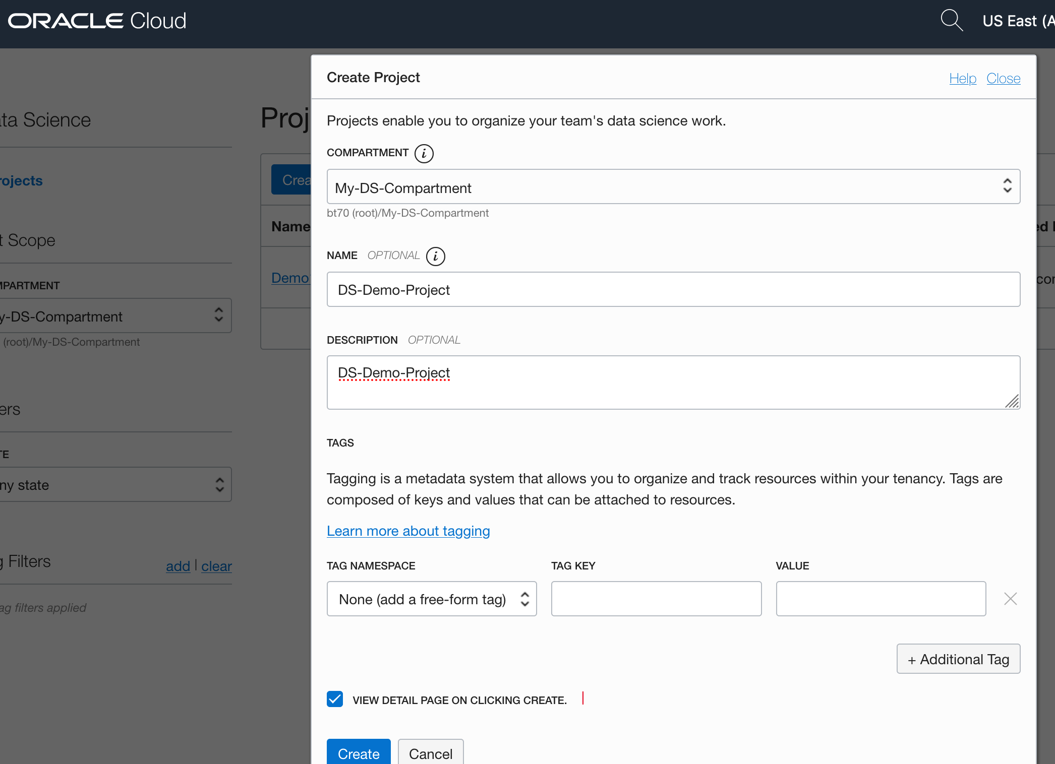

That’s the Project created.
2 – Create a Notebook
After creating a project (see above) you can not create one or many Notebook Sessions.
To create a Notebook Session click on the Create Notebook Session button (see the above image). This will create a VM to contain your notebook and associated work. Just like all VM in Oracle Cloud, they come in various different shapes. These can be adjusted at a later time to scale up and then back down based on the work you will be performing.
The following example creates a Notebook Session using the basic VM shape. I call the Notebook ‘DS-Demo-Notebook’. I also set the Block Storage size to 50G, which is the minimum value. The VNC details have been defaulted to those assigned to the Compartment. Click Create button at the bottom of the page.

The Notebook Session VM will be created. This might take a few minutes. When created you will see a screen like the following.

3 – Open the Notebook
After completing the above steps you can now open the Notebook Session in your browser. Either click on the Open button (see above image), or copy the link and share with your data science team.
Important: There are a few important considerations when using the Notebooks. While the session is running you will be paying for it, even if the session got terminated at the browser or you lost connect. To manage costs, you may need to stop the Notebook session. More details on this in a later post.
After clicking on the Open button, a new browser tab will open and will ask you to log-in.

After logging in you will see your Notebook.
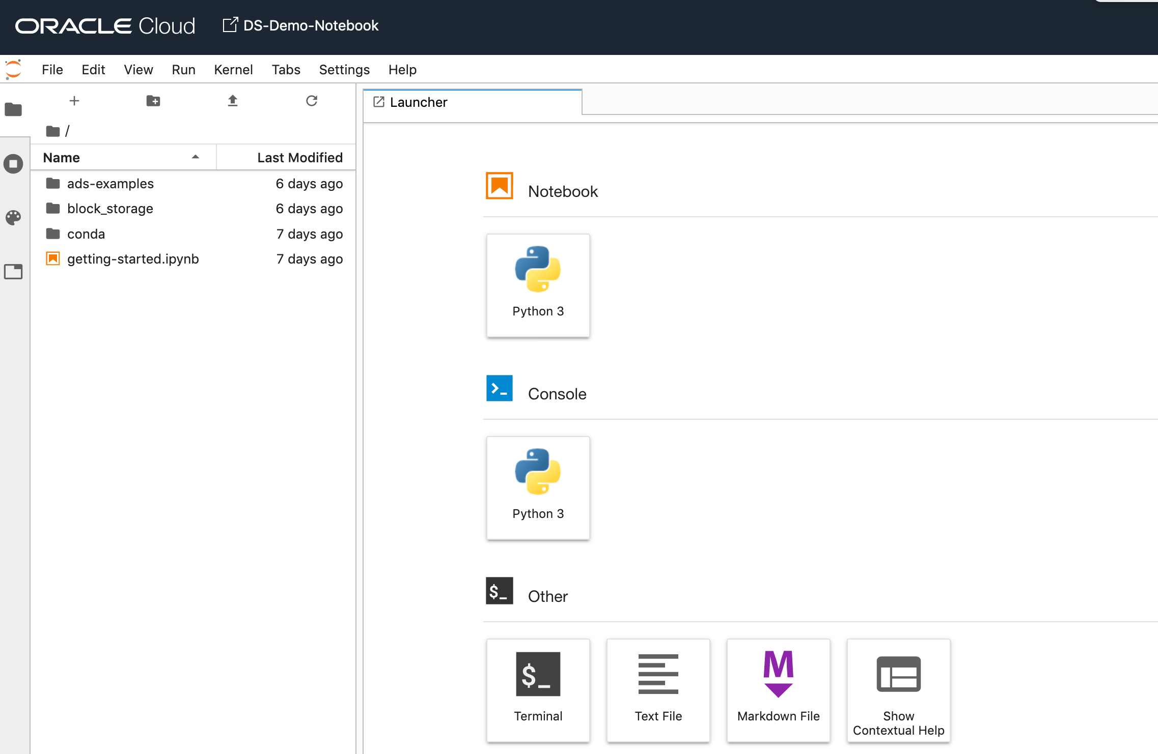
4 – Explore the Notebook Environment
The Notebook comes pre-loaded with lots of goodies.
The menu on the left-hand side provides a directory with lots of sample Notebooks, access to the block storage and a sample getting started Notebook.

When you are ready to create your own Notebook you can click on the icon for that.

Or if you already have a Notebook, created elsewhere, you can load that into your OCI Data Science environment.

The uploaded Notebook will appear in the list on the left-hand side of the screen.
Creating a VM on Oracle Always Free
I’m going to create a new Cloud VM to host some of my machine learning work. The first step is to create the VM before installing the machine learning software.
That’s what I’m going to do in this blog post and the next blog post. In this blog post I’ll step through how to setup the VM using the Oracle Always Free cloud offering. In the next I’ll go through the machine learning software install and setup.
Step 1 – Create a ssh key/file
Whatever your preferred platform for your day to day computer there will be software available for you to generate a ssh key file. You will need this when creating the VM and for when you want to login in to VM on the command line. My day-to-day workhorse is a Mac, and I used the following command to create the ssh key file.
ssh-keygen -t rsa -N "" -b 2048 -C "myOracleCloudkey" -f myOracleCloudkey
Step 2 – Login and Select create VM
Log into your Oracle Cloud Always Free account.

Select Create a VM Instance.

Step 3 – Configure the VM
Give the instance a name. I called mine ‘b01-vm-1‘
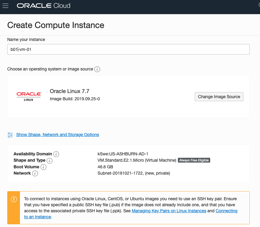
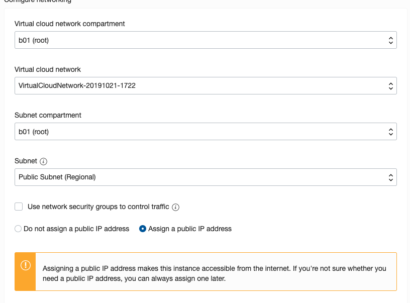
Expand the networks section by clicking on Show Shape, Network and Storage Options. Set the IP address to be public.
Scroll down to the ssh section. Select the ssh file you created earlier.
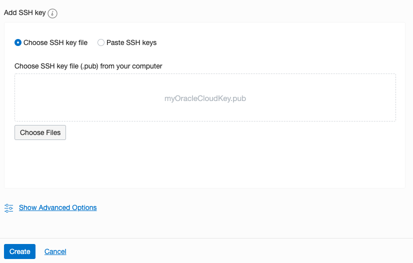
Click on the Create button.
That’s it, all done. Just wait for the VM to be created. This will takes a few seconds.
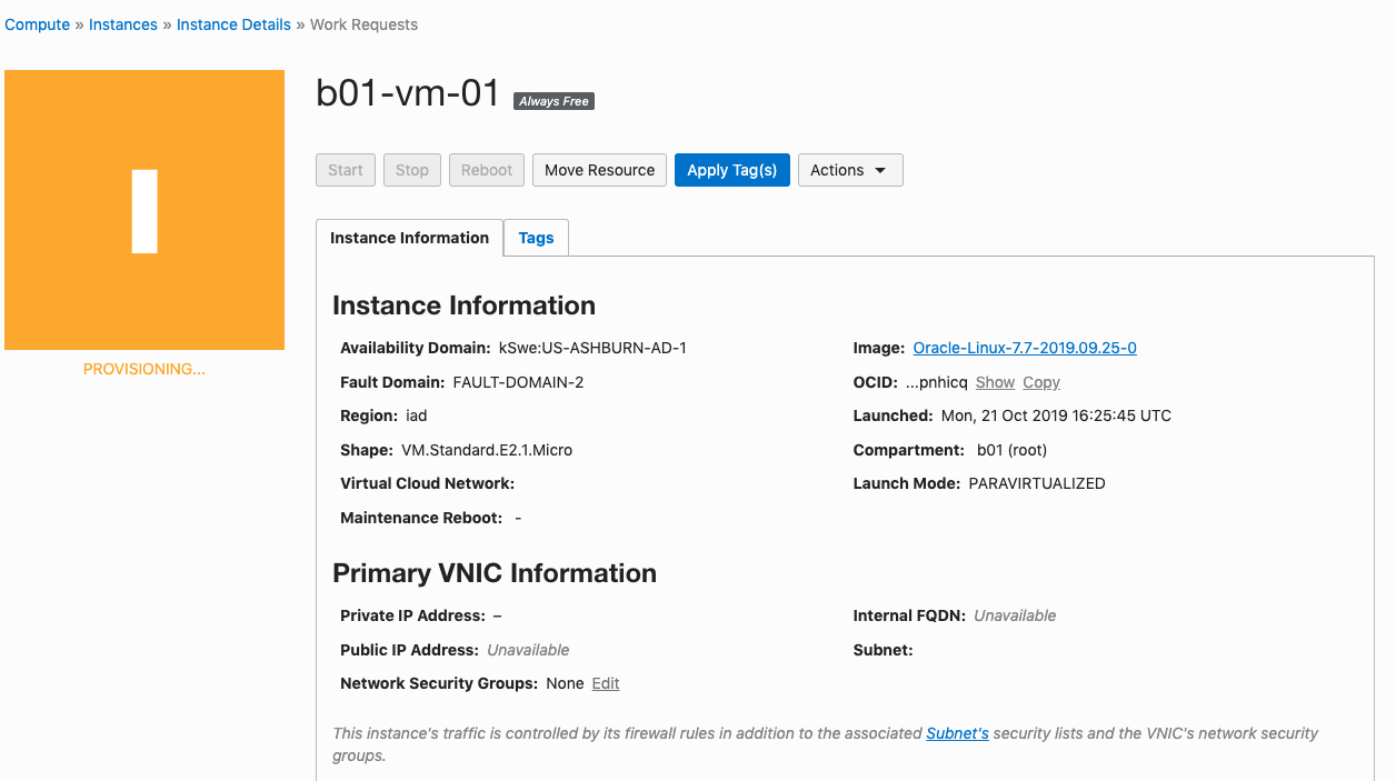
After the VM is created the IP address will be listed on this screen. Take note of it.
Step 4 – Connect and log into the VM
We can not log into the VM using ssh, to prove that it exists, using the command
ssh -i <name of ssh file> opc@<ip address of VM>
When I use this command I get the following:
ssh -i XXXXXXXXXX opc@XXX.XXX.XXX.XXX
The authenticity of host 'XXX.XXX.XXX.XXX (XXX.XXX.XXX.XXX)' can't be established.
ECDSA key fingerprint is SHA256:fX417Z1yFoQufm7SYfxNi/RnMH5BvpvlOb2gOgnlSCs.
Are you sure you want to continue connecting (yes/no)? yes
Warning: Permanently added 'XXX.XXX.XXX.XXX' (ECDSA) to the list of known hosts.
Enter passphrase for key 'XXXXXXXXXX':
[opc@b1-vm-01 ~]$ pwd
/home/opc

[opc@b1-vm-01 ~]$ df
Filesystem   1K-blocks     Used Available Use%  Mounted on
devtmpfs        469092        0    469092   0%  /dev
tmpfs           497256        0    497256   0%  /dev/shm
tmpfs           497256     6784    490472   2%  /run
tmpfs           497256        0    497256   0%  /sys/fs/cgroup
/dev/sda3     40223552  1959816  38263736   5%  /
/dev/sda1       204580     9864    194716   5%  /boot/efi
tmpfs            99452        0     99452   0%  /run/user/1000
And there we have it. A VM setup on Oracle Always Free.
Next step is to install some Machine Learning software.
ADW – Loading data using Object Storage
There are a number of different ways to load data into your Autonomous Data Warehouse (ADW) environment. I’ll have posts about these alternatives.
In this blog post I’ll go through the steps needed to load data using Object Storage. This might appear to have a large-ish number of steps, but once you have gone through it and have some of the parts already setup and configuration from your first time, then the second and subsequent times will be easier.
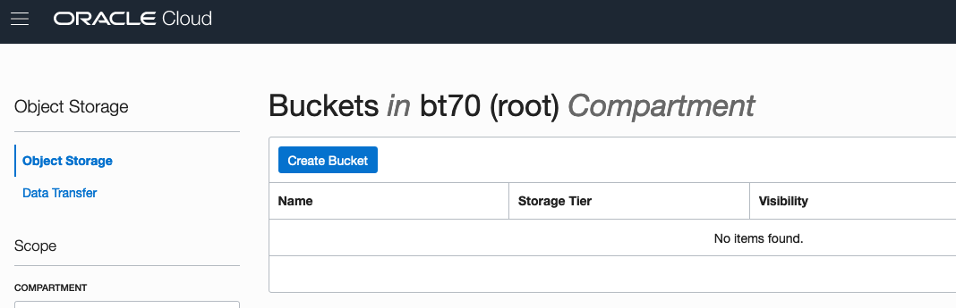
After logging into your Oracle Cloud dashboard, select Object Storage from the side menu.

Then click on the Create Bucket button.
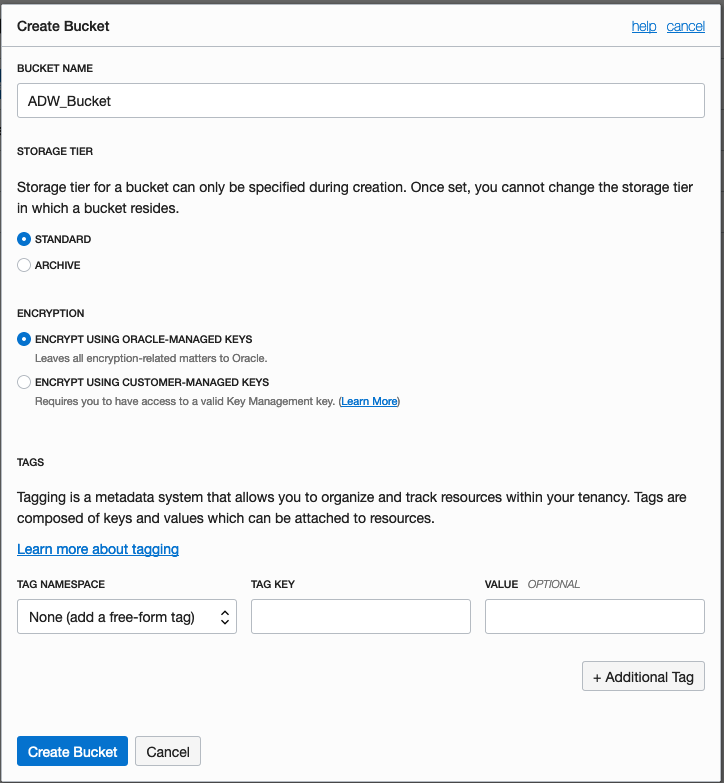
Enter a name for the Object Storage bucket, take the defaults for the for the rest, and click on the Create Bucket button at the bottom. In my example, I’ve called the bucket ‘ADW_Bucket’.
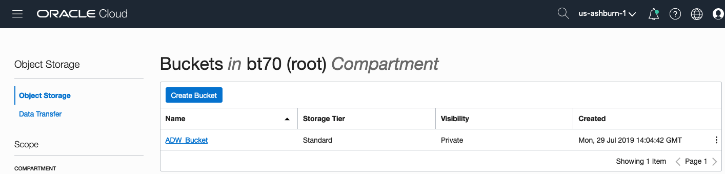
Click on the name of the bucket in the list.
And then click Upload Objects button.

In the Upload Objects window, browse for the file(s) you want to upload.


Then click on the Upload Objects button on the Upload Objects window. After a few moments you will see a message saying the file(s) have been uploaded. Click on the Close window.

Click into the Object details and take a note/copy of the URL Path. You will need this later
To load data from the Oracle Cloud Infrastructure(OCI) Object Storage you will need an OCI user with the appropriate privileges to read data (or upload) data to the Object Store. The communication between the database and the object store relies on the Swift protocol and the OCI user Auth Token. Go back to the menu in the upper left and select users.


Then click on the user name to view the details. This is probably your OCI username.
On the left hand side of the page click Auth Tokens, and then click on Generate Token button. Give a name for the token e.g ADW_TOKEN, and then generate token.

Save the generated token to use later.

Open SQL Developer and setup a connection to your OML User/schema. When connected the next steps is to authenticate with the Object storage using your OCI username and the Auth Token, generated above.
BEGIN
  DBMS_CLOUD.CREATE_CREDENTIAL(
    credential_name => 'ADW_TOKEN',
    username => '<your cloud username>',
    password => '<generated auth token>'
  );
END;
If successful you should get the following message. If not then you probably entered something incorrectly. Go back and review the previous steps
PL/SQL procedure successfully completed.
Next, create a table to store the data you want to import. For my table the create table is the following. [It is one of the sample data sets for OML, and I’ve made the create table statement compact to save space in this post]
create table credit_scoring_100k
( customer_id number(38,0), age number(4,0), income number(38,0), marital_status varchar2(26 byte),
number_of_liables number(3,0), wealth varchar2(4000 byte), education_level varchar2(26 byte),
tenure number(4,0), loan_type varchar2(26 byte), loan_amount number(38,0),
loan_length number(5,0), gender varchar2(26 byte), region varchar2(26 byte),
current_address_duration number(5,0), residental_status varchar2(26 byte),
number_of_prior_loans number(3,0), number_of_current_accounts number(3,0),
number_of_saving_accounts number(3,0), occupation varchar2(26 byte),
has_checking_account varchar2(26 byte), credit_history varchar2(26 byte),
present_employment_since varchar2(26 byte), fixed_income_rate number(4,1),
debtor_guarantors varchar2(26 byte), has_own_phone_no varchar2(26 byte),
has_same_phone_no_since number(4,0), is_foreign_worker varchar2(26 byte),
number_of_open_accounts number(3,0), number_of_closed_accounts number(3,0),
number_of_inactive_accounts number(3,0), number_of_inquiries number(3,0),
highest_credit_card_limit number(7,0), credit_card_utilization_rate number(4,1),
delinquency_status varchar2(26 byte), new_bankruptcy varchar2(26 byte),
number_of_collections number(3,0), max_cc_spent_amount number(7,0),
max_cc_spent_amount_prev number(7,0), has_collateral varchar2(26 byte),
family_size number(3,0), city_size varchar2(26 byte), fathers_job varchar2(26 byte),
mothers_job varchar2(26 byte), most_spending_type varchar2(26 byte),
second_most_spending_type varchar2(26 byte), third_most_spending_type varchar2(26 byte),
school_friends_percentage number(3,1), job_friends_percentage number(3,1),
number_of_protestor_likes number(4,0), no_of_protestor_comments number(3,0),
no_of_linkedin_contacts number(5,0), average_job_changing_period number(4,0),
no_of_debtors_on_fb number(3,0), no_of_recruiters_on_linkedin number(4,0),
no_of_total_endorsements number(4,0), no_of_followers_on_twitter number(5,0),
mode_job_of_contacts varchar2(26 byte), average_no_of_retweets number(4,0),
facebook_influence_score number(3,1), percentage_phd_on_linkedin number(4,0),
percentage_masters number(4,0), percentage_ug number(4,0),
percentage_high_school number(4,0), percentage_other number(4,0),
is_posted_sth_within_a_month varchar2(26 byte), most_popular_post_category varchar2(26 byte),
interest_rate number(4,1), earnings number(4,1), unemployment_index number(5,1),
production_index number(6,1), housing_index number(7,2), consumer_confidence_index number(4,2),
inflation_rate number(5,2), customer_value_segment varchar2(26 byte),
customer_dmg_segment varchar2(26 byte), customer_lifetime_value number(8,0),
churn_rate_of_cc1 number(4,1), churn_rate_of_cc2 number(4,1),
churn_rate_of_ccn number(5,2), churn_rate_of_account_no1 number(4,1),
churn_rate__of_account_no2 number(4,1), churn_rate_of_account_non number(4,2),
health_score number(3,0), customer_depth number(3,0),
lifecycle_stage number(38,0), credit_score_bin varchar2(100 byte));
After creating the table, you are ready to import the data from Object storage. To do this you will need to use the DBMS_COULD PL/SQL package.
begin
   dbms_cloud.copy_data(
   table_name =>'credit_scoring_100k',
   credential_name =>'ADW_TOKEN',
   file_uri_list => '<url of file in your Object Store bucket, see comment earlier in post>',
   format => json_object('ignoremissingcolumns' value 'true', 'removequotes' value 'true', 'dateformat' value 'YYYY-MM-DD HH24:MI:SS', 'blankasnull' value 'true', 'delimiter' value ',', 'skipheaders' value '1')
);
end;
All done.
You can now query the data and use with Oracle Machine Learning, etc.
[I said at the top of the post there are other methods available. More on this in other posts]
GoLang: Inserting records into Oracle Database using goracle
In this blog post I’ll give some examples of how to process data for inserting into a table in an Oracle Database. I’ve had some previous blog posts on how to setup and connecting to an Oracle Database, and another on retrieving data from an Oracle Database and the importance of setting the Array Fetch Size.
When manipulating data the statements can be grouped (generally) into creating new data and updating existing data.
When working with this kind of processing we need to avoid the creation of the statements as a concatenation of strings. This opens the possibility of SQL injection, plus we are not allowing the optimizer in the database to do it’s thing. Prepared statements allows for the reuse of execution plans and this in turn can speed up our data processing and applications.
In a previous blog post I gave a simple example of a prepared statement for querying data and then using it to pass in different values as a parameter to this statement.
dbQuery, err := db.Prepare("select cust_first_name, cust_last_name, cust_city from sh.customers where cust_gender = :1")
if err != nil {
    fmt.Println(err)
    return
}
defer dbQuery.Close()

rows, err := dbQuery.Query('M')
if err != nil {
    fmt.Println(".....Error processing query")
    fmt.Println(err)
    return
}
defer rows.Close()

var CustFname, CustSname,CustCity string
for rows.Next() {
    rows.Scan(&CustFname, &CustSname, &CustCity)
    fmt.Println(CustFname, CustSname, CustCity)
}
For prepared statements for inserting data we can follow a similar structure. In the following example a table call LAST_CONTACT is used. This table has columns:
- CUST_ID
- CON_METHOD
- CON_MESSAGE
_, err := db.Exec("insert into LAST_CONTACT(cust_id, con_method, con_message) VALUES(:1, :2, :3)", 1, "Phone", "First contact with customer")
if err != nil {
    fmt.Println(".....Error Inserting data")
    fmt.Println(err)
    return
}
an alternative is the following and allows us to get some additional information about what was done and the result from it. In this example we can get the number records processed.
stmt, err := db.Prepare("insert into LAST_CONTACT(cust_id, con_method, con_message) VALUES(:1, :2, :3)")
if err != nil {
    fmt.Println(err)
    return
}

res, err := dbQuery.Query(1, "Phone", "First contact with customer")
if err != nil {
    fmt.Println(".....Error Inserting data")
    fmt.Println(err)
    return
}

rowCnt := res.RowsAffected()
fmt.Println(rowCnt, " rows inserted.")
A similar approach can be taken for updating and deleting records
Managing Transactions
With transaction, a number of statements needs to be processed as a unit. For example, in double entry book keeping we have two inserts. One Credit insert and one debit insert. To do this we can define the start of a transaction using db.Begin() and the end of the transaction with a Commit(). Here is an example were we insert two contact details.
// start the transaction
transx, err := db.Begin()
if err != nil {
    fmt.Println(err)
    return
}

// Insert first record
_, err := db.Exec("insert into LAST_CONTACT(cust_id, con_method, con_message) VALUES(:1, :2, :3)", 1, "Email", "First Email with customer")
if err != nil {
    fmt.Println(".....Error Inserting data - first statement")
    fmt.Println(err)
    return
}
// Insert second record
_, err := db.Exec("insert into LAST_CONTACT(cust_id, con_method, con_message) VALUES(:1, :2, :3)", 1, "In-Person", "First In-Person with customer")
if err != nil {
    fmt.Println(".....Error Inserting data - second statement")
    fmt.Println(err)
    return
}

// complete the transaction
err = transx.Commit()
if err != nil {
    fmt.Println(".....Error Committing Transaction")
    fmt.Println(err)
    return
}
GoLang: Querying records from Oracle Database using goracle
Continuing my series of blog posts on using Go Lang with Oracle, in this blog I’ll look at how to setup a query, run the query and parse the query results. I’ll give some examples that include setting up the query as a prepared statement and how to run a query and retrieve the first record returned. Another version of this last example is a query that returns one row.
Check out my previous post on how to create a connection to an Oracle Database.
Let’s start with a simple example. This is the same example from the blog I’ve linked to above, with the Database connection code omitted.
    dbQuery := "select table_name from user_tables where table_name not like 'DM$%' and table_name not like 'ODMR$%'"
    rows, err := db.Query(dbQuery)
    if err != nil {
        fmt.Println(".....Error processing query")
        fmt.Println(err)
        return
    }
    defer rows.Close()

    fmt.Println("... Parsing query results")
    var tableName string
    for rows.Next() {
        rows.Scan(&tableName)
        fmt.Println(tableName)
    }
Processing a query and it’s results involves a number of steps and these are:
- Using Query() function to send the query to the database. You could check for errors when processing each row
- Iterate over the rows using Next()
- Read the columns for each row into variables using Scan(). These need to be defined because Go is strongly typed.
- Close the query results using Close(). You might want to defer the use of this function but depends if the query will be reused. The result set will auto close the query after it reaches the last records (in the loop). The Close() is there just in case there is an error and cleanup is needed.
You should never use * as a wildcard in your queries. Always explicitly list the attributes you want returned and only list the attributes you want/need. Never list all attributes unless you are going to use all of them. There can be major query performance benefits with doing this.
Now let us have a look at using prepared statement. With these we can parameterize the query giving us greater flexibility and reuse of the statements. Additionally, these give use better query execution and performance when run the the database as the execution plans can be reused.
    dbQuery, err := db.Prepare("select cust_first_name, cust_last_name, cust_city from sh.customers where cust_gender = :1")
    if err != nil {
        fmt.Println(err)
        return
    }
    defer dbQuery.Close()

    rows, err := dbQuery.Query('M')
    if err != nil {
        fmt.Println(".....Error processing query")
        fmt.Println(err)
        return
    }
    defer rows.Close()

    var CustFname, CustSname,CustCity string
    for rows.Next() {
        rows.Scan(&CustFname, &CustSname, &CustCity)
        fmt.Println(CustFname, CustSname, CustCity)
    }
Sometimes you may have queries that return only one row or you only want the first row returned by the query. In cases like this you can reduce the code to something like the following.
var CustFname, CustSname,CustCity string
err := db.Prepare("select cust_first_name, cust_last_name, cust_city from sh.customers where cust_gender = ?").Scan(&CustFname, &CustSname, &CustCity)
if err != nil {
    fmt.Println(err)
    return
}
fmt.Println(CustFname, CustSname, CustCity)
or an alternative to using Quer(), use QueryRow()
dbQuery, err := db.Prepare("select cust_first_name, cust_last_name, cust_city from sh.customers where cust_gender = ?")
if err != nil {
    fmt.Println(err)
    return
}
defer dbQuery.Close()

var CustFname, CustSname,CustCity string
err := dbQuery.QueryRow('M').Scan(&CustFname, &CustSname, &CustCity)
if err != nil {
    fmt.Println(".....Error processing query")
    fmt.Println(err)
    return
}
fmt.Println(CustFname, CustSname, CustCity)
Importance of setting Fetched Rows size for Database Query using Golang
When issuing queries to the database one of the challenges every developer faces is how to get the results quickly. If your queries are only returning a small number of records, eg. < 5, then you don’t really have to worry about execution time. That is unless your query is performing some complex processing, joining lots of tables, etc.
Most of the time developers are working with one or a small number of records, using a simple query. Everything runs quickly.
But what if your query is returning several tens or thousands of records. Assuming we have a simple query and no query optimization is needed, the challenge facing the developer is how can you get all of those records quickly into your environment and process them. Typically the database gets blamed for the query result set being returned slowly. But what if this wasn’t the case? In most cases developers take the default parameter settings of the functions and libraries. For database connection libraries and their functions, you can change some of the parameters and affect how your code, your query, gets executed on the Database server and can affect how quickly the data is shipped from the database to your code.
One very important parameter to consider is the query array size. This is the number of records the database will send to your code in each batch. The database will keep sending batches until you tell it to stop. It makes sense to have the size of this batch set to a small value, as most queries return one or a small number of records. But when we get onto returning a larger number of records it can affect the response time significantly.
I tested the effect of changing the size of the returning buffer/array using Golang and querying data in an Oracle Database, hosted on Oracle Cloud, and using goracle library to connect to the database.
[ I did a similar test using Python. The results can be found here. You will notices that Golang is significantly quicker than Python, as you would expect. ]
The database table being queried contains 55,000 records and I just executed a SELECT * FROM … on this table. The results shown below contain the timing the query took to process this data for different buffer/array sizes by setting the FetchRowCount value.
rows, err := db.Query(dbQuery, goracle.FetchRowCount(arraySize))

As you can see, as the size of the buffer/array size increases the timing it takes to process the data drops. This is because the buffer/array is returning a larger number of records, and this results in a reduced number of round trips to/from the database i.e. fewer packets of records are sent across the network.
The challenge for the developer is to work out the optimal number to set for the buffer/array size. The default for the goracle libary, using Oracle client is 256 row/records.
When that above query is run, without the FetchRowCount setting, it will use this default 256 value. When this is used we get the following timings.
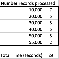
We can see, for the data set being used in this test case the optimal setting needs to be around 1,500.
What if we set the parameter to be very large? That would no necessarily make it quicker. You can see from the first table the timing starts to increase for the last two settings. There is an overhead in gathering and sending the data.
Here is a subset of the Golang code I used to perform the tests.
var currentTime = time.Now()

var i int

var custId int

arrayOne := [11] int{5, 10, 30, 50, 100, 200, 500, 1000, 1500, 2000, 2500}


currentTime = time.Now()


fmt.Println("Array Size = ", arraySize, " : ", currentTime.Format("03:04:05:06 PM"))


for index, arraySize := range arrayOne {

    currentTime = time.Now()

    fmt.Println(index, " Array Size = ", arraySize, " : ", currentTime.Format("03:04:05:06 PM"))


    db, err := sql.Open("goracle", username+"/"+password+"@"+host+"/"+database)

    if err != nil {

        fmt.Println("... DB Setup Failed")

        fmt.Println(err)

        return

    }

    defer db.Close()


    if err = db.Ping(); err != nil {

        fmt.Printf("Error connecting to the database: %s\n", err)

        return

    }


    currentTime = time.Now()

    fmt.Println("...Executing Query", currentTime.Format("03:04:05:06 PM"))

    dbQuery := "select cust_id from sh.customers"

    rows, err := db.Query(dbQuery, goracle.FetchRowCount(arraySize))

    if err != nil {

        fmt.Println(".....Error processing query")

        fmt.Println(err)

        return

    }

    defer rows.Close()


    i = 0

    currentTime = time.Now()

    fmt.Println("... Parsing query results", currentTime.Format("03:04:05:06 PM"))

   for rows.Next() {

        rows.Scan(&custId)

        i++

        if i% 10000 == 0 {

            currentTime = time.Now()

            fmt.Println("...... ",i, " customers processed", currentTime.Format("03:04:05:06 PM"))

        }

    }


    currentTime = time.Now()

    fmt.Println(i, " customers processed", currentTime.Format("03:04:05:06 PM"))


    fmt.Println("... Closing connection")

    finishTime := time.Now()

    fmt.Println("Finished at ", finishTime.Format("03:04:05:06 PM"))


}

You must be logged in to post a comment.