
Python
Oracle Object Storage – Buckets & Loading files
In a previous post, I showed what you need to do to setup your local PC/laptop to be able to connect to OCI. I also showed how to perform some simple queries on your Object Storage environment. Go check out that post before proceeding with the examples in this blog.
- Oracle Object Storage – Setup and Explore
- Oracle Object Storage – Buckets & Loading files
- Oracle Object Storage – Downloading and Deleting
- Oracle Object Storage – Parallel Uploading
In this post, I’ll build upon my previous post by giving some Python functions to:
- Check if Bucket exists
- Create a Buckets
- Delete a Bucket
- Upload an individual file
- Upload an entire directory
Let’s start with a function to see if a Bucket already exists.
def check_bucket_exists(b_name):
    #check if Bucket exists
    is_there = False
    l_b = object_storage_client.list_buckets(NAMESPACE, COMPARTMENT_ID).data
    for bucket in l_b:
        if bucket.name == b_name:
            is_there = True

    if is_there == True:
        print(f'Bucket {b_name} exists.')
    else:
        print(f'Bucket {b_name} does not exist.')

    return is_there
A simple test for a bucket called ‘DEMO_bucket’. This was defined in a variable previously (see previous post). I’ll use this ‘DEMO_bucket’ throughout these examples.
b_exists = check_bucket_exists(BUCKET_NAME)
print(b_exists)

---
Bucket DEMO_Bucket does not exist.
False
Next we can more onto a function for creating a Bucket.
def create_bucket(b):
    #create Bucket if it does not exist
    bucket_exists = check_bucket_exists(b)
    if bucket_exists == False:
        try:
            create_bucket_response = object_storage_client.create_bucket(
                NAMESPACE,
                oci.object_storage.models.CreateBucketDetails(
                    name=demo_bucket_name,
                    compartment_id=COMPARTMENT_ID
                )
            )
            bucket_exists = True
            # Get the data from response
            print(f'Created Bucket {create_bucket_response.data.name}')
        except Exception as e:
            print(e.message)
    else:
        bucket_exists = True
        print(f'... nothing to create.')

    return bucket_exists
A simple test for a bucket called ‘DEMO_bucket’. This was defined in a variable previously (see previous post).
b_exists = create_bucket(BUCKET_NAME)
---
Bucket DEMO_Bucket does not exist.
Created Bucket DEMO_Bucket
Next, let’s delete a Bucket and any files stored in it.
def delete_bucket(b_name):
    bucket_exists = check_bucket_exists(b_name)
    objects_exist = False
    if bucket_exists == True:
        print('Starting - Deleting Bucket '+b_name)
        print('... checking if objects exist in Bucket (bucket needs to be empty)')
        try:
            object_list = object_storage_client.list_objects(NAMESPACE, b_name).data
            objects_exist = True
        except Exception as e:
            objects_exist = False

        if objects_exist == True:
            print('... ... Objects exists in Bucket. Deleting these objects.')
            count = 0
            for o in object_list.objects:
                count+=1
                object_storage_client.delete_object(NAMESPACE, b_name, o.name)

            if count > 0:
                print(f'... ... Deleted {count} objects in {b_name}')
            else:
                print(f'... ... Bucket is empty. No objects to delete.')

        else:
            print(f'... No objects to delete, Bucket {b_name} is empty')


        print(f'... Deleting bucket {b_name}')
        response = object_storage_client.delete_bucket(NAMESPACE, b_name)
        print(f'Deleted bucket {b_name}')
The example output below shows what happens when I’ve already loaded data into the Bucket (which I haven’t shown in the examples so far – but I will soon).
delete_bucket(BUCKET_NAME)

---
Bucket DEMO_Bucket exists.
Starting - Deleting Bucket DEMO_Bucket
... checking if objects exist in Bucket (bucket needs to be empty)
... ... Objects exists in Bucket. Deleting these objects.
... ... Bucket is empty. No objects to delete.
... Deleting bucket DEMO_Bucket
Deleted bucket DEMO_Bucket
Now that we have our functions for managing Buckets, we can now have a function for uploading a file to a bucket.
def upload_file(b, f):
    file_exists = os.path.isfile(f)
    if file_exists == True:
        #check to see if Bucket exists
        b_exists = check_bucket_exists(b)
        if b_exists == True:
            print(f'... uploading {f}')
            try:
                object_storage_client.put_object(NAMESPACE, b, os.path.basename(f), io.open(f,'rb'))
                print(f'. finished uploading {f}')
            except Exception as e:
                print(f'Error uploading file. Try again.')
                print(e)
        else:
            print('... Create Bucket before uploading file.')

    else:
        print(f'... File {f} does not exist or cannot be found. Check file name and full path')
Just select a file from your computer and give the full path to that file and the Bucket name.
up_file = '/Users/brendan.tierney/Dropbox/bill.xls'
upload_file(BUCKET_NAME, up_file)

---
Bucket DEMO_Bucket does not exist.
... Create Bucket before uploading file.
Our final function is an extended version of the previous one. This function takes a Directory path and uploads all the files to the Bucket.
def upload_directory(b, d):
    count = 0

    #check to see if Bucket exists
    b_exists = check_bucket_exists(b)
    if b_exists == True:
        #loop files
        for filename in os.listdir(d):
            print(f'... uploading {filename}')
            try:
                object_storage_client.put_object(NAMESPACE, b, filename, io.open(os.path.join(d,filename),'rb'))
                count += 1
            except Exception as e:
                print(f'... ... Error uploading file. Try again.')
                print(e)

    else:
        print('... Create Bucket before uploading files.')

    if count == 0:
        print('... Empty directory. No files uploaded.')
    else:
        print(f'Finished uploading Directory : {count} files into {b} bucket')
and to call it …
up_directory = '/Users/brendan.tierney/Dropbox/OCI-Vision-Images/Blue-Peter/'
upload_directory(BUCKET_NAME, up_directory)

---
Bucket DEMO_Bucket exists.
... uploading thumbnail_IMG_2336.jpg
... uploading .DS_Store
... uploading 2017-08-31 19.46.42.jpg
... uploading thumbnail_IMG_2333.jpg
... uploading 347397087_620984963239631_2131524631626484429_n.jpg
... uploading thumbnail_IMG_1712.jpg
... uploading thumbnail_IMG_1711.jpg
... uploading 2017-11-22 20.18.58.jpg
... uploading thumbnail_IMG_1710.jpg
... uploading 2018-12-03 11.04.57.jpg
... uploading IMG_6779.jpg
... uploading oug_ire18_1.jpg
... uploading 2017-10-16 13.13.20.jpg
... uploading IMG_2347.jpg
Finished uploading Directory : 14 files into DEMO_Bucket bucket
Oracle Object Storage – Setup and Explore
This blog post will walk you through how to access Oracle OCI Object Storage and explore what buckets and files you have there, using Python and the OCI Python library. There will be additional posts which will walk through some of the other typical tasks you’ll need to perform with moving files into and out of OCI Object Storage.
- Oracle Object Storage – Buckets & Loading files
- Oracle Object Storage – Downloading and Deleting
- Oracle Object Storage – Parallel Uploading
The first thing you’ll need to do is to install the OCI Python library. You can do this by running pip command or if using Anaconda using their GUI for doing this. For example,
pip3 install ociCheck out the OCI Python documentation for more details.
Next, you’ll need to get and setup the configuration settings and download the pem file.
We need to create the config file that will contain the required credentials and information for working with OCI. By default, this file is stored in : ~/.oci/config
mkdir ~/oci
cd oci
Now create the config file, using vi or something similar.
vi config
Edit the file to contain the following, but look out for the parts that need to be changed/updated to match your OCI account details.
[ADMIN_USER]user=ocid1.user.oc1..<unique_ID>
fingerprint=<your_fingerprint>
tenancy = ocid1.tenancy.oc1..<unique_ID>
region = us-phoenix-1key_file=
<path to key .pem file>
The above details can be generated by creating an API key for your OCI user. Copy and paste the default details to the config file.
- [ADMIN_USER] > you can name this anything you want, but it will referenced in Python.
- user > enter the user ocid. OCID is the unique resource identifier that OCI provides for each resource.
- fingerprint > refers to the fingerprint of the public key you configured for the user.
- tenancy > your tenancy OCID.
- region > the region that you are subscribed to.
- key_file > the path to the .pem file you generated.

Just download the .pem file and the config file details. Add them to the config file, and give the full path to the .epm file, including its name.
You are now ready to use the OCI Python library to access and use your OCI cloud environment. Let’s run some tests to see if everything works and connects ok.
#import libraries
import oci
import json
import os
import io

#load the config file
config = oci.config.from_file("~/.oci/config")
config

#only part of the output is displayed due to security reasons
{'log_requests': False, 'additional_user_agent': '', 'pass_phrase': None, 'user': 'oci...........
We can now define some core variables.
#My Compartment ID
COMPARTMENT_ID = "ocid1.tenancy.oc1..............

#Object storage Namespace
object_storage_client = oci.object_storage.ObjectStorageClient(config)
NAMESPACE = object_storage_client.get_namespace().data

#Name of Bucket for this demo
BUCKET_NAME = 'DEMO_Bucket'
We can now define some functions to:
- List the Buckets in my OCI account
- List the number of files in each Bucket
- Number of files in a particular Bucket
- Check for Bucket Existence
def list_buckets():
    l_buckets = object_storage_client.list_buckets(NAMESPACE, COMPARTMENT_ID).data
    # Get the data from response
    for bucket in l_buckets:
        print(bucket.name)

def list_bucket_counts():
    l_buckets = object_storage_client.list_buckets(NAMESPACE, COMPARTMENT_ID).data
    for bucket in l_buckets:
        print("Bucket name: ",bucket.name)
        buck_name = bucket.name
        objects = object_storage_client.list_objects(NAMESPACE, buck_name).data
        count = 0
        for i in objects.objects:
            count+=1

        print('... num of objects :', count)

def check_bucket_exists(b_name):
    #check if Bucket exists
    is_there = False
    l_b = object_storage_client.list_buckets(NAMESPACE, COMPARTMENT_ID).data
    for bucket in l_b:
        if bucket.name == b_name:
            is_there = True

    if is_there == True:
        print(f'Bucket {b_name} exists.')
    else:
        print(f'Bucket {b_name} does not exist.')

    return is_there

def list_bucket_details(b):
    bucket_exists = check_bucket_exists(b)
    if bucket_exists == True:
        objects = object_storage_client.list_objects(NAMESPACE, b).data
        count = 0
        for i in objects.objects:
            count+=1

        print(f'Bucket {b} has objects :', count)
Now we can run these functions to test them. Before running these make sure you can create a connection to OCI.

Changing/Increasing Cell Width in Juypter Notebook
When working with Jupyter Notebook you might notice the cell width can vary from time to time, and mostly when you use different screens, with different resolutions.
This can make your code appear slightly odd on the screen with only a certain amount being used. You can of into the default settings to change the sizing, but this might not suit in most cases.
It would be good to be able to adjust this dynamically. In such a situation, you can use one of the following options.
The first option is to use the IPython option to change the display settings. This first example adjusts everything (menu, toolbar and cells) to 50% of the screen width.
from IPython.display import display, HTML
display(HTML("<style>.container { width:50% !important; }</style>"))
This might not give you the result you want, but it helps to illustrate how to use this command. By changing the percentage, you can get a better outcome. For example, by changing the percentage to 100%.
from IPython.display import display, HTML
display(HTML("<style>.container { width:100% !important; }</style>"))
Keep a careful eye on making these changes, as I’ve found Jupyter stops responding to these changes. A quick refresh of the page will reset everything back to the default settings. Then just run the command you want.
An alternative is to make the changes to the CSS.
from IPython.display import display, HTML

display(HTML(data="""
<style>
    div#notebook-container    { width: 95%; }
    div#menubar-container     { width: 65%; }
    div#maintoolbar-container { width: 99%; }
</style>
"""))
You might want to change those percentages to 100%.
If we need to make the changes permanent we can locate the CSS file: custom.css. Depending on your system it will be located in different places.
For Linux and virtual environments have a look at the following directories.
~/.jupyter/custom/custom.css
Machine Learning App Migration to Oracle Cloud VM
Over the past few years, I’ve been developing a Stock Market prediction algorithm and made some critical refinements to it earlier this year. As with all analytics, data science, machine learning and AI projects, testing is vital to ensure its performance, accuracy and sustainability. Taking such a project out of a lab environment and putting it into a production setting introduces all sorts of different challenges. Some of these challenges include being able to self-manage its own process, logging, traceability, error and event management, etc. Automation is key and implementing all of these extra requirements tasks way more code and time than developing the actual algorithm. Typically, the machine learning and algorithms code only accounts for less than five percent of the actual code, and in some cases, it can be less than one percent!
I’ve come to the stage of deploying my App to a production-type environment, as I’ve been running it from my laptop and then a desktop for over a year now. It’s now 100% self-managing so it’s time to deploy. The environment I’ve chosen is using one of the Virtual Machines (VM) available on the Oracle Free Tier. This means it won’t cost me a cent (dollar or more) to run my App 24×7.
My App has three different components which use a core underlying machine learning predictions engine. Each is focused on a different set of stock markets. These marks operate in the different timezone of US markets, European Markets and Asian Markets. Each will run on a slightly different schedule than the rest.
The steps outlined below take you through what I had to do to get my App up and running the VM (Oracle Free Tier). It took about 20 minutes to complete everything
The first thing you need to do is create a ssh key file. There are a number of ways of doing this and the following is an example.
ssh-keygen -t rsa -N "" -b 2048 -C "myOracleCloudkey" -f myOracleCloudkey
This key file will be used during the creation of the VM and for logging into the VM.
Log into your Oracle Cloud account and you’ll find the Create Instances Compute i.e. create a virtual machine/

Complete the Create Instance form and upload the ssh file you created earlier. Then click the Create button. This assumes you have networking already created.

It will take a minute or two for the VM to be created and you can monitor the progress.
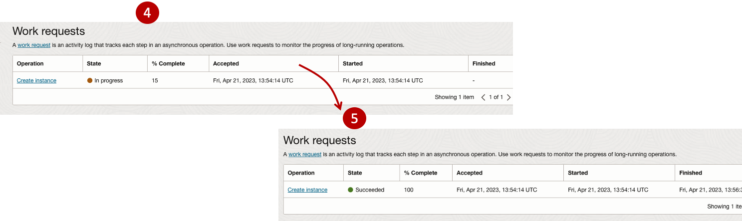
After it has been created you need to click on the start button to start the VM.
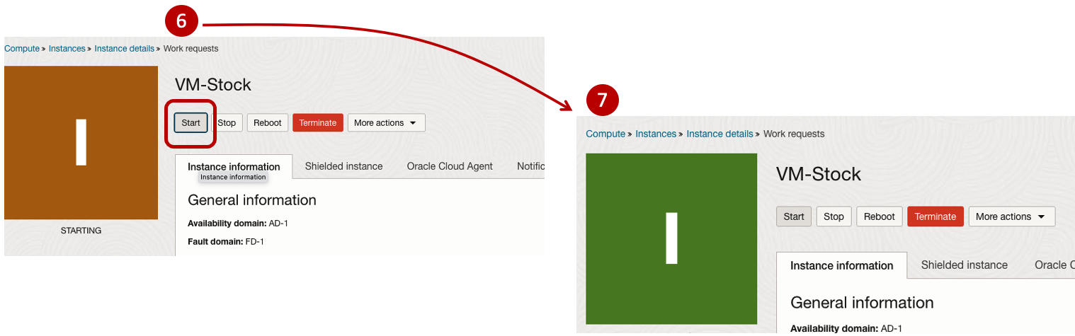
After it has started you can now log into the VM from a terminal window, using the public IP address
ssh -i myOracleCloudKey opc@xxx.xxx.xxx.xxxAfter you’ve logged into the VM it’s a good idea to run an update.
[opc@vm-stocks ~]$ sudo yum -y update
Last metadata expiration check: 0:13:53 ago on Fri 21 Apr 2023 14:39:59 GMT.
Dependencies resolved.
========================================================================================================================
 Package                         Arch       Version                                          Repository            Size
========================================================================================================================
Installing:
 kernel-uek                      aarch64    5.15.0-100.96.32.el8uek                          ol8_UEKR7            1.4 M
 kernel-uek-core                 aarch64    5.15.0-100.96.32.el8uek                          ol8_UEKR7             47 M
 kernel-uek-devel                aarch64    5.15.0-100.96.32.el8uek                          ol8_UEKR7             19 M
 kernel-uek-modules              aarch64    5.15.0-100.96.32.el8uek                          ol8_UEKR7             59 M
Upgrading:
 NetworkManager                  aarch64    1:1.40.0-6.0.1.el8_7                             ol8_baseos_latest    2.1 M
 NetworkManager-config-server    noarch     1:1.40.0-6.0.1.el8_7                             ol8_baseos_latest    141 k
 NetworkManager-libnm            aarch64    1:1.40.0-6.0.1.el8_7                             ol8_baseos_latest    1.9 M
 NetworkManager-team             aarch64    1:1.40.0-6.0.1.el8_7                             ol8_baseos_latest    156 k
 NetworkManager-tui              aarch64    1:1.40.0-6.0.1.el8_7                             ol8_baseos_latest    339 k
...
...
The VM is now ready to setup and install my App. The first step is to install Python, as all my code is written in Python.
[opc@vm-stocks ~]$ sudo yum install -y python39
Last metadata expiration check: 0:20:35 ago on Fri 21 Apr 2023 14:39:59 GMT.
Dependencies resolved.
========================================================================================================================
 Package                         Architecture  Version                                        Repository           Size
========================================================================================================================
Installing:
 python39                        aarch64       3.9.13-2.module+el8.7.0+20879+a85b87b0         ol8_appstream        33 k
Installing dependencies:
 python39-libs                   aarch64       3.9.13-2.module+el8.7.0+20879+a85b87b0         ol8_appstream       8.1 M
 python39-pip-wheel              noarch        20.2.4-7.module+el8.6.0+20625+ee813db2         ol8_appstream       1.1 M
 python39-setuptools-wheel       noarch        50.3.2-4.module+el8.5.0+20364+c7fe1181         ol8_appstream       497 k
Installing weak dependencies:
 python39-pip                    noarch        20.2.4-7.module+el8.6.0+20625+ee813db2         ol8_appstream       1.9 M
 python39-setuptools             noarch        50.3.2-4.module+el8.5.0+20364+c7fe1181         ol8_appstream       871 k
Enabling module streams:
 python39                                      3.9

Transaction Summary
========================================================================================================================
Install  6 Packages

Total download size: 12 M
Installed size: 47 M
Downloading Packages:
(1/6): python39-pip-20.2.4-7.module+el8.6.0+20625+ee813db2.noarch.rpm                    23 MB/s | 1.9 MB     00:00
(2/6): python39-pip-wheel-20.2.4-7.module+el8.6.0+20625+ee813db2.noarch.rpm             5.5 MB/s | 1.1 MB     00:00
...
...
Next copy the code to the VM, setup the environment variables and create any necessary directories required for logging. The final part of this is to download the connection Wallett for the Database. I’m using the Python library oracledb, as this requires no additional setup.
Then install all the necessary Python libraries used in the code, for example, pandas, matplotlib, tabulate, seaborn, telegram, etc (this is just a subset of what I needed). For example here is the command to install pandas.
pip3.9 install pandasAfter all of that, it’s time to test the setup to make sure everything runs correctly.
The final step is to schedule the App/Code to run. Before setting the schedule just do a quick test to see what timezone the VM is running with. Run the date command and you can see what it is. In my case, the VM is running GMT which based on the current time locally, the VM was showing to be one hour off. Allowing for this adjustment and for day-light saving time, the time +/- markets openings can be set. The following example illustrates setting up crontab to run the App, Monday-Friday, between 13:00-22:00 and at 5-minute intervals. Open crontab and edit the schedule and command. The following is an example
> contab -e

*/5 13-22 * * 1-5 python3.9 /home/opc/Stocks.py >Stocks.txt
For some stock market trading apps, you might want it to run more frequently (than every 5 minutes) or less frequently depending on your strategy.
After scheduling the components for each of the Geographic Stock Market areas, the instant messaging of trades started to appear within a couple of minutes. After a little monitoring and validation checking, it was clear everything was running as expected. It was time to sit back and relax and see how this adventure unfolds.
For anyone interested, the App does automated trading with different brokers across the markets, while logging all events and trades to an Oracle Autonomous Database (Free Tier = no cost), and sends instant messages to me notifying me of the automated trades. All I have to do is Nothing, yes Nothing, only to monitor the trade notifications. I mentioned earlier the importance of testing, and with back-testing of the recent changes/improvements (as of the date of post), the App has given a minimum of 84% annual return each year for the past 15 years. Most years the return has been a lot more!
Image Augmentation (Pencil & Cartoon) with OpenCV #SYM42
OpenCV has been with us for over two decades and provides us with a rich open-source library for performing image processing.
In this post I’m going to illustrate how you can use it to convert images (of people) into pencil sketches and cartoon images. As with most examples you find on such technologies there are things it is good at and some things this isn’t good at. Using the typical IT phrase, “It Depends” comes into play with image processing. What might work with one set of images, might not work as well with others.
The example images below consist of the Board of a group called SYM42, or Symposium42. Yes, they said I could use their images and show the output from using OpenCV 🙂 This group was formed by a community to support the community, was born out of an Oracle Community but is now supporting other technologies. They are completely independent of any Vendor which means they can be 100% honest about which aspects of any product do or do not work and are not influenced by the current sales or marketing direction of any company. Check out their About page.
Let’s get started. After downloading the images to process, let’s view them.
import cv2
import matplotlib.pyplot as plt
import numpy as np

dir = '/Users/brendan.tierney/Dropbox/6-Screen-Background/'
file = 'SYM42-Board-Martin.jpg'

image = cv2.imread(dir+file)
img_name = 'Original Image'
#Show the image with matplotlib
#plt.imshow(image)

#OpenCV uses BGR color scheme whereas matplotlib uses RGB colors scheme
#convert BGR image to RGB by using the following
plt.imshow(cv2.cvtColor(image, cv2.COLOR_BGR2RGB))
plt.axis(False)
plt.show()

I’m using Jupyter Notebooks for this work. In the above code, you’ll see I’ve commented out the line [#plt.imshow(image)]. This comment doesn’t really work in Jupyter Notebooks and instead you need to swap to using Matplotlib to display the images
To convert to a pencil sketch, we need to convert to pencil sketch, apply a Gaussian Blur, invert the image and perform bit-wise division to get the final pencil sketch.
#convert to grey scale
#cvtColor function
grey_image = cv2.cvtColor(image, cv2.COLOR_BGR2GRAY)
#invert the image
invert_image = cv2.bitwise_not(grey_image)

#apply Gaussian Blue : adjust values until you get pencilling effect required
blur_image=cv2.GaussianBlur(invert_image, (21,21),0)  #111,111

#Invert Blurred Image
#Repeat previous step
invblur_image=cv2.bitwise_not(blur_image)

#The sketch can be obtained by performing bit-wise division between
# the grayscale image and the inverted-blurred image.
sketch_image=cv2.divide(grey_image, invblur_image, scale=256.0)

#display the pencil sketch
plt.imshow(cv2.cvtColor(sketch_image, cv2.COLOR_BGR2RGB))
plt.axis(False)
plt.show()
The following code listing contains the same as above and also includes the code to convert to a cartoon style.
import os
import glob
import cv2
import matplotlib.pyplot as plt
import numpy as np

def edge_mask(img, line_size, blur_value):
  gray = cv2.cvtColor(img, cv2.COLOR_BGR2GRAY)
  gray_blur = cv2.medianBlur(gray, blur_value)
  edges = cv2.adaptiveThreshold(gray_blur, 255, cv2.ADAPTIVE_THRESH_MEAN_C, cv2.THRESH_BINARY, line_size, blur_value)
  return edges

def cartoon_image(img_cartoon):
    img=img_cartoon

    line_size = 7
    blur_value = 7
    edges = edge_mask(img, line_size, blur_value)

    #Clustering - (K-MEANS)
    imgf=np.float32(img).reshape(-1,3)
    criteria=(cv2.TERM_CRITERIA_EPS+cv2.TERM_CRITERIA_MAX_ITER,20,1.0)
    compactness,label,center=cv2.kmeans(imgf,5,None,criteria,10,cv2.KMEANS_RANDOM_CENTERS)
    center=np.uint8(center)
    final_img=center[label.flatten()]
    final_img=final_img.reshape(img.shape)

    cartoon=cv2.bitwise_and(final_img,final_img,mask=edges)

    return cartoon

def sketch_image(image_file, blur):
    import_image = cv2.imread(image_file)

    #cvtColor function
    grey_image = cv2.cvtColor(import_image, cv2.COLOR_BGR2GRAY)
    #invert the image
    invert_image = cv2.bitwise_not(grey_image)

    blur_image=cv2.GaussianBlur(invert_image, (blur,blur),0)   #111,111

    #Invert Blurred Image
    #Repeat previous step
    invblur_image=cv2.bitwise_not(blur_image)

    sketch_image=cv2.divide(grey_image, invblur_image, scale=256.0)
    cartoon_img=cartoon_image(import_image)

    #plot images
#    plt.figure(figsize=(9,6))
    plt.rcParams["figure.figsize"] = (12,8)

    #plot cartoon
    plt.subplot(1,3,3)
    plt.imshow(cv2.cvtColor(cartoon_img, cv2.COLOR_BGR2RGB))
    plt.title('Cartoon Image', size=12, color='red')
    plt.axis(False)

    #plot sketch
    plt.subplot(1,3,2)
    plt.imshow(cv2.cvtColor(sketch_image, cv2.COLOR_BGR2RGB))
    plt.title('Sketch Image', size=12, color='red')
    plt.axis(False)
    #plot original image
    plt.subplot(1,3,1)
    plt.imshow(cv2.cvtColor(import_image, cv2.COLOR_BGR2RGB))
    plt.title('Original Image', size=12, color='blue')
    plt.axis(False)

    #plot show
    plt.show()

for filepath in glob.iglob(dir+'SYM42-Board*.*'):
    #print(filepath)
    #import_image = cv2.imread(dir+file)
    sketch_image(filepath, 23)
For the SYM42 Board members, we get the following output.


As you can see from these images, some are converted in a way you would expect. While others seem to give little effect.
Thanks to the Board of SYM42 for allowing me to use their images.
Morse Code with Python
Morse code is a method used in telecommunication to encode text characters as standardized sequences of two different signal duration, called dots and dashes. Morse code is named after Samuel Morse, one of the inventors of the telegraph (wikipedia).
The example code below illustrates taking input from the terminal, converting it into Morse code, playing the Morse code sound signal, then converts the Morse code back into plain text and prints this to the screen. This is a base set of code you can use and can be easily extended to make it more interactive.
When working with sound and audio in Python there are lots of different libraries available for this. But some of the challenges is trying to pick a suitable one, and one that is still supported in more recent times. One of the most commonly referenced library is called Winsound, but that is for Windows based computers. Not everyone uses Windows machines, just like myself using a Mac. So Winsound wasn’t an option. I selected to use the playsound library, mainly based on how commonly referenced it is.
To play the dots and dashs, I needed some sound files and these were originally sources from Wikimedia. The sound files are available on wikimedia, but these come in ogg file formats. I’ve converted the dot and dash files to mp3 files and theses can be downloaded from here, dot download and dash download. I also included a Error sound file in my code for when an error occurs! Error download.
When you download the code and sound files, you might need to adjust the timing for playing the Morse code sound files, as this might be dependent on your computer
The Morse code mapping was setup as a dictionary and a reverse mapping of this dictionary was used to translate morse code into plain text.
import time
from playsound import playsound

toMorse = {'a': ".-",    'b': "-...",
           'c': "-.-.",  'd': "-..",
           'e': ".",     'f': "..-.",
           'g': "--.",   'h': "....",
           'i': "..",    'j': ".---",
           'k': "-.-",   'l': ".-..",
           'm': "--",    'n': "-.",
           'o': "---",   'p': ".--.",
           'q': "--.-",  'r': ".-.",
           's': "...",   't': "-",
           'u': "..-",   'v': "...-",
           'w': ".--",   'x': "-..-",
           'y': "-.--",  'z': "--..",
           '1': ".----", '2': "..---",
           '3': "...--", '4': "....-",
           '5': ".....", '6': "-....",
           '7': "--...", '8': "---..",
           '9': "----.", '0': "-----",
           ' ': " ",   '.': ".-.-.-",
           ',': "--..--", '?': "..--..",
           "'": ".----.", '@': ".--.-.",
           '-': "-....-", '"': ".-..-.",
           ':': "---...", ';': "---...",
           '=': "-...-",  '!': "-.-.--",
           '/': "-..-.",  '(': "-.--.",
           ')': "-.--.-", 'á': ".--.-",
           'é': "..-.."}

#sounds from https://commons.wikimedia.org/wiki/Morse_code
soundPath = "/Users/brendan.tierney/Dropbox/4-Datasets/morse_code_audio/"
#adjust this value to change time between dots/dashes
tBetween = 0.1

def play_morse_beep():
    playsound(soundPath + 'Dot_morse_code.mp3')
    time.sleep(1 * tBetween)

def play_morse_dash():
    playsound(soundPath + 'Dash_morse_code.mp3')
    time.sleep(2 * tBetween)

def play_morse_space():
    time.sleep(2 * tBetween)

def play_morse_error():
    playsound(soundPath + 'Error_invalid_char.mp3')
    time.sleep(2 * tBetween)

def text_to_morse(inStr):
    mStr = ""
    for c in [x for x in inStr]:
        m = toMorse[c]
        mStr += m + ' '

    print("morse=",mStr)
    return mStr

def play_morse(inMorse):
    for m in inMorse:
        if m == ".":
            play_morse_beep()
        elif m == "-":
            play_morse_dash()
        elif m == " ":
            play_morse_space()
        else:
            play_morse_error()

#Get Input Text
from colorama import Fore, Back, Style

print(Fore.RED + '')

inputStr = input("Enter text -> morse :").lower() #.strip()
print(Fore.BLACK + '' + inputStr)

mStr = text_to_morse(inputStr)
play_morse(mStr)

play_morse(mStr)
Then to reverse the Morse code.
#reverse the k,v
mToE = {}
for key, value in toMorse.items():
        mToE[value] = key

def morse_to_english(inStr):
    inStr = inStr.split(" ")
    engStr = []
    for c in inStr:
        if c in mToE:
            engStr.append(mToE[c])

    return "".join(engStr)

x=morse_to_english(mStr)
print(x)Automated Data Visualizations in Python
Creating data visualizations in Python can be a challenge. For some it an be easy, but for most (and particularly new people to the language) they always have to search for the commands in the documentation or using some search engine. Over the past few years we have seem more and more libraries coming available to assist with many of the routine and tedious steps in most data science and machine learning projects. I’ve written previously about some data profiling libraries in Python. These are good up to a point, but additional work/code is needed to explore the data to suit your needs. One of these Python libraries, designed to make your initial work on a new data set easier is called AutoViz. It’s good to see there is continued development work on this library, which can be really help for creating initial sets of charts for all the variables in your data set, plus it has some additional features which help to make it very useful and cuts down on some of the additional code you might need to write.
The outputs from AutoViz are very extensive, and are just too long to show in this post. The images below will give you an indication of what if typically generated. I’d encourage you to install the library and run it on one of your data sets to see the full extent of what it can do. For this post, I’ll concentrate on some of the commands/parameters/settings to get the most out of AutoViz.
Firstly there is the install via pip command or install using Anaconda.
pip3 install autovizFor comparison purposes I’m going to use the same data set as I’ve used in the data profiling post (see above). Here’s a quick snippet from that post to load the data and perform the data profiling (see post for output)
import pandas as pd
import pandas_profiling as pp

#load the data into a pandas dataframe
df = pd.read_csv("/Users/brendan.tierney/Downloads/Video_Games_Sales_as_at_22_Dec_2016.csv")
We can not skip to using AutoViz. It supports the loading and analzying of data sets direct from a file or from a pandas dataframe. In the following example I’m going to use the dataframe (df) created above.
from autoviz import AutoViz_Class

AV = AutoViz_Class()
df2 = AV.AutoViz(filename="", dfte=df)  #for a file, fill in the filename and remove dfte parameter
This will analyze the data and create lots and lots of charts for you. Some are should in the following image. One the helpful features is the ‘data cleaning improvements’ section where it has performed a data quality assessment and makes some suggestions to improve the data, maybe as part of the data preparation/cleaning step.

There is also an option for creating different types of out put with perhaps the Bokeh charts being particularly useful.
chart_format='bokeh': interactive Bokeh dashboards are plotted in Jupyter Notebooks.chart_format='server', dashboards will pop up for each kind of chart on your web browser.chart_format='html', interactive Bokeh charts will be silently saved as Dynamic HTML files underAutoViz_Plotsdirectory
df2 = AV.AutoViz(filename="", dfte=df, chart_format='bokeh')
The next example allows for the report and charts to be focused on a particular dependent or target variable, particular in scenarios where classification will be used.
df2 = AV.AutoViz(filename="", dfte=df, depVar="Platform")
A little warning when using this library. It can take a little bit of time for it to run and create all the different charts. On the flip side, it save you from having to write lots and lots of code!
Migrating SAS files to CSV and database
Many organizations have been using SAS Software to analyse their data for many decades. As with most technologies organisations will move to alternative technologies are some point. Recently I’ve experienced this kind of move. In doing so any data stored in one format for the older technology needed to be moved or migrated to the newer technology. SAS Software can process data in a variety of format, one of which is their own internal formats. Thankfully Pandas in Python as a function to read such SAS files into a pandas dataframe, from which it can be saved into some alternative format such as CSV. The following code illustrates this conversion, where it will migrate all the SAS files in a particular directory, converts them to CSV and saves the new file in a destination directory. It also copies any existing CSV files to the new destination, while ignore any other files. The following code is helpful for batch processing of files.
import os
import pandas as pd

#define the Source and Destination directories
source_dir='/Users/brendan.tierney/Dropbox/4-Datasets/SAS_Data_Sets'
dest_dir=source_dir+'/csv'

#What file extensions to read and convert
file_ext='.sas7bdat'

#Create output directory if it does not already exist
if not os.path.exists(dest_dir):
    os.mkdir(dest_dir)
else:  #If directory exists, delete all files
    for filename in os.listdir(source_dir):
        os.remove(filename)

#Process each file
for filename in os.listdir(source_dir):
    #Process the SAS file
    if filename.endswith(file_ext):
        print('.processing file :',filename)
        print('...converting file to csv')
        df=pd.read_sas(os.path.join(source_dir, filename))
        df.to_csv(os.path.join(dest_dir, filename))
        print('.....finished creating CSV file')
    elif filename.endswith('csv'):
        #Copy any CSV files to the Destination Directory
        print('.copying CSV file')
        cmd_copy='cp '+os.path.join(source_dir, filename)+' '+os.path.join(dest_dir, filename)
        os.system(cmd_copy)
        print('.....finished copying CSV file')
    else:
        #Ignore any other type of files
        print('.ignoring file :',filename)

print('--Finished--')
That’s it. All the files have now been converted and located in the destination directory.
For most, the above might be all you need, but sometimes you’ll need to move the the newer technology. In most cases the newer technology will easily use the CSV files. But in some instance your final destination might be a database. In my scenarios I use the CSV2DB app developed by Gerald Venzi. You can download the code from GitHub. You can use this to load CSV files into Oracle, MySQL, PostgreSQL, SQL Server and Db2 databases. Here’s and example of the command line to load into an Oracle Database.
csv2db load -f /Users/brendan.tierney/Dropbox/4-Datasets/SAS_Data_Sets/csv -t pva97nk -u analytics -p analytics -d PDB1
Preparing images for #DeepLearning by removing background
There are a number of methods available for preparing images for input to a variety of purposes. For example, for input to deep learning, other image processing models/applications/systems, etc. But sometimes you just need a quick tool to perform a certain task. An example of this is I regularly have to edit images to extract just a certain part of it, or to filter out all the background colors and/or objects etc. There are a a variety of tools available to help you with this kind of task. For me, I’m a Mac user, so I use the instant alpha feature available in some of the Mac products. But what if you are not a Mac user, what can you use.
I’ve recently come across a very useful Python library that takes all or most of the hard work out of doing such tasks, and has proved to be extremely useful for some demos and projects I’ve been working on. The Python library I’m using is remgb (Remove Background). It isn’t perfect, but it does a pretty good job and only in a small number of modified images, did I need to do some additional processing.
Let’s get started with setting things up to use remgb. I did encounter some minor issues installing it, and I’ve give the workarounds below, just in case you encounter the same.
pip3 install remgbThis will install lots of required libraries and will check for compatibility with what you have installed. The first time I ran the install it generated some errors. It also suggested I update my version of pip, which I did, then uninstalled the remgb library and installed again. No errors this time.
When I ran the code below, I got some errors about accessing a document on google drive or it had reached the maximum number of views/downloads. The file it is trying to access is an onix model. If you click on the link, you can download the file. Create a directory called .u2net (in your home directory) and put the onix file into it. Make sure the directory is readable. After doing that everything runs smoothly for me.
The code I’ve given below is typical of what I’ve been doing on some projects. I have a folder with lots of images where I want to remove the background and only keep the key foreground object. Then save the modified images to another directory. It is these image that can be used in products like Amazon Rekognition, Oracle AI Services, and lots of other similar offerings.
from rembg import remove
from PIL import Image
import os
from colorama import Fore, Back, Style

sourceDir = '/Users/brendan.tierney/Dropbox/4-Datasets/F1-Drivers/'
destDir = '/Users/brendan.tierney/Dropbox/4-Datasets/F1-Drivers-NewImages/'

print('Searching = ', sourceDir)

files = os.listdir(sourceDir)
for file in files:
    try:
        inputFile = sourceDir + file
        outputFile = destDir + file

        with open(inputFile, 'rb') as i:
            print(Fore.BLACK + '..reading file : ', file)
            input = i.read()
            print(Fore.CYAN + '...removing background...')
            output = remove(input)

        try:
            with open(outputFile, 'wb') as o:
                print(Fore.BLUE + '.....writing file : ', outputFile)
                o.write(output)
        except:
            print(Fore.RED + 'Error writing file :', outputFile)

except:
    print(Fore.RED + 'Error processing file :', file)

print(Fore.BLACK + '---')
print(Fore.BLACK + 'Finished processing all files')
print(Fore.BLACK + '---')
For this demonstration I’ve used images of the F1 drivers for 2022. I had collected five images of each driver with different backgrounds including, crowds, pit-lane, giving media interviews, indoor and outdoor images.
Generally the results were very good. Here are some results with the before and after.


As you can see from these image there are some where a shadow remains and the library wasn’t able to remove it. The following images gives some additional examples of this. The first is with Bottas and his car, where the car wasn’t removed. The second driver is Vettel where the library captures his long hair and keeps it in the filtered image.


CAO Points 2022 – Grade inflation, deflation or in-line
Last week I wrote a blog post analysing the Leaving Cert results over the past 3-8 years. Part of that post also looked at the claim from the Dept of Education saying the results in 2022 would be “in-line on aggregate” with the results from 2021. The outcome of the analysis was grade deflation was very evident in many subjects, but when analysed and profiled at a very high level, they did look similar.
I didn’t go into how that might impact on the CAO (Central Applications Office) Points. If there was deflation in some of the core and most popular subjects, then you might conclude there could be some changes in the profile of CAO Points being awarded, and that in turn would have a small change on the CAO Points needed for a lot of University courses. But not all of them, as we saw last week, the increased number of students who get grades in the H4-H7 range. This could mean a small decrease in points for courses in the 520+ range, and a small increase in points needed in the 300-500-ish range.
The CAO have published the number of students of each 10 point range. I’ve compared the 2022 data, with each year going back to 2015. The following table is a high level summary of the results in 50 point ranges.
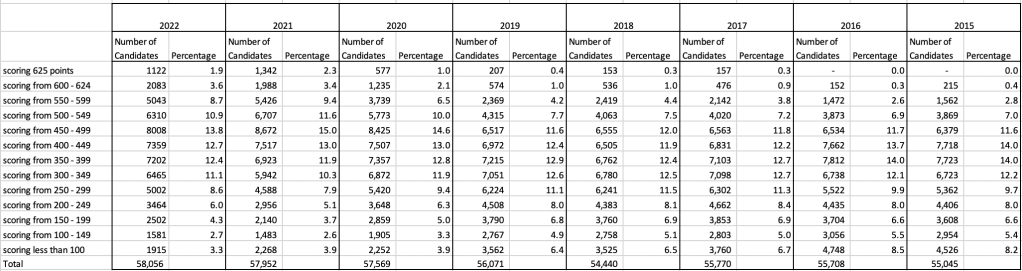
An initial look at these numbers and percentages might look like points are similar to last year and even 2020. But for 2015-2019 the similarity is closer. Again looking back at the previous blog post, we can see the results profiles for 20215-2019 are broadly similar and does indicate some normalisation might have been happening each year. The following chart illustrate the percentage of students who achieved points in each range.
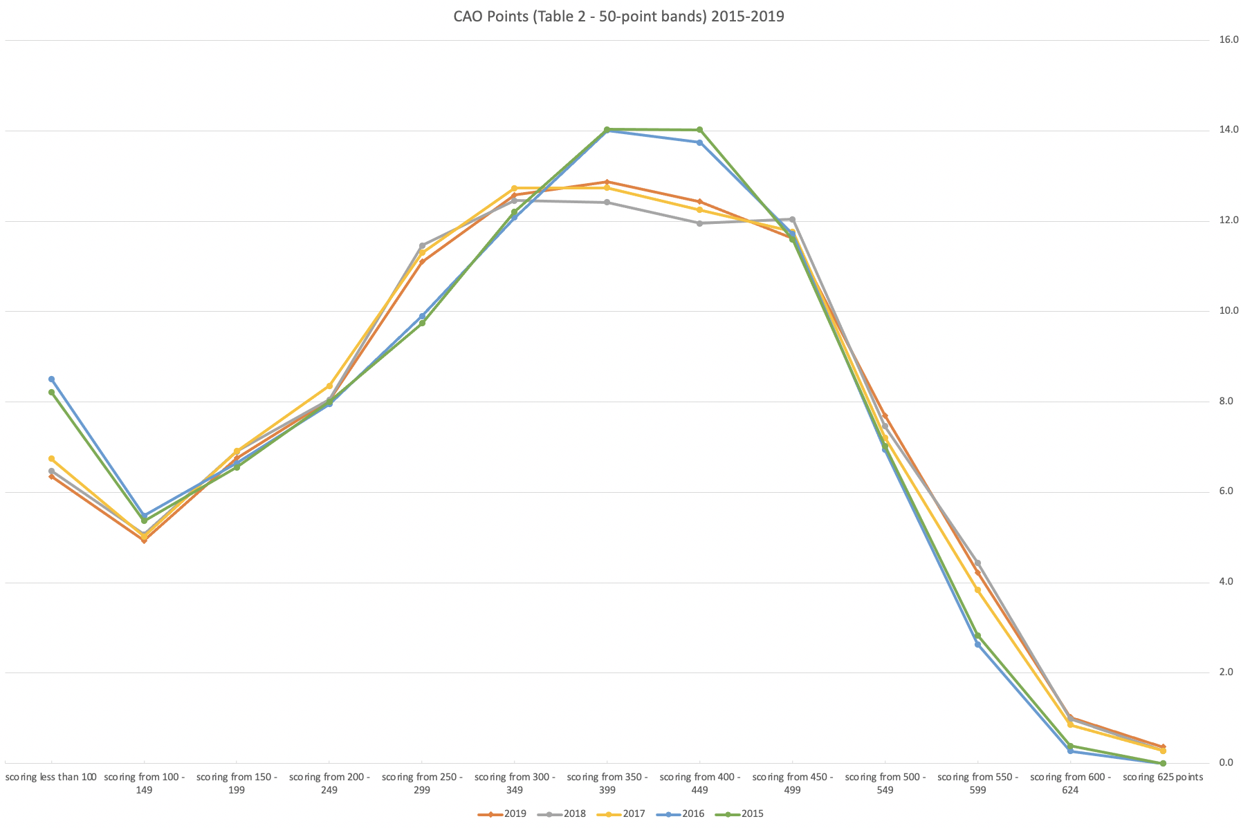
From the above we can see the profile is similar across 2015-2019, although there does seem to be a flattening of the curve between 2015-2016!
Let’s now have a look at 2019 (the last pre-coivd year), 2021 and 2022. This will allow use to compare the “inflated” years to the last “normal” year.
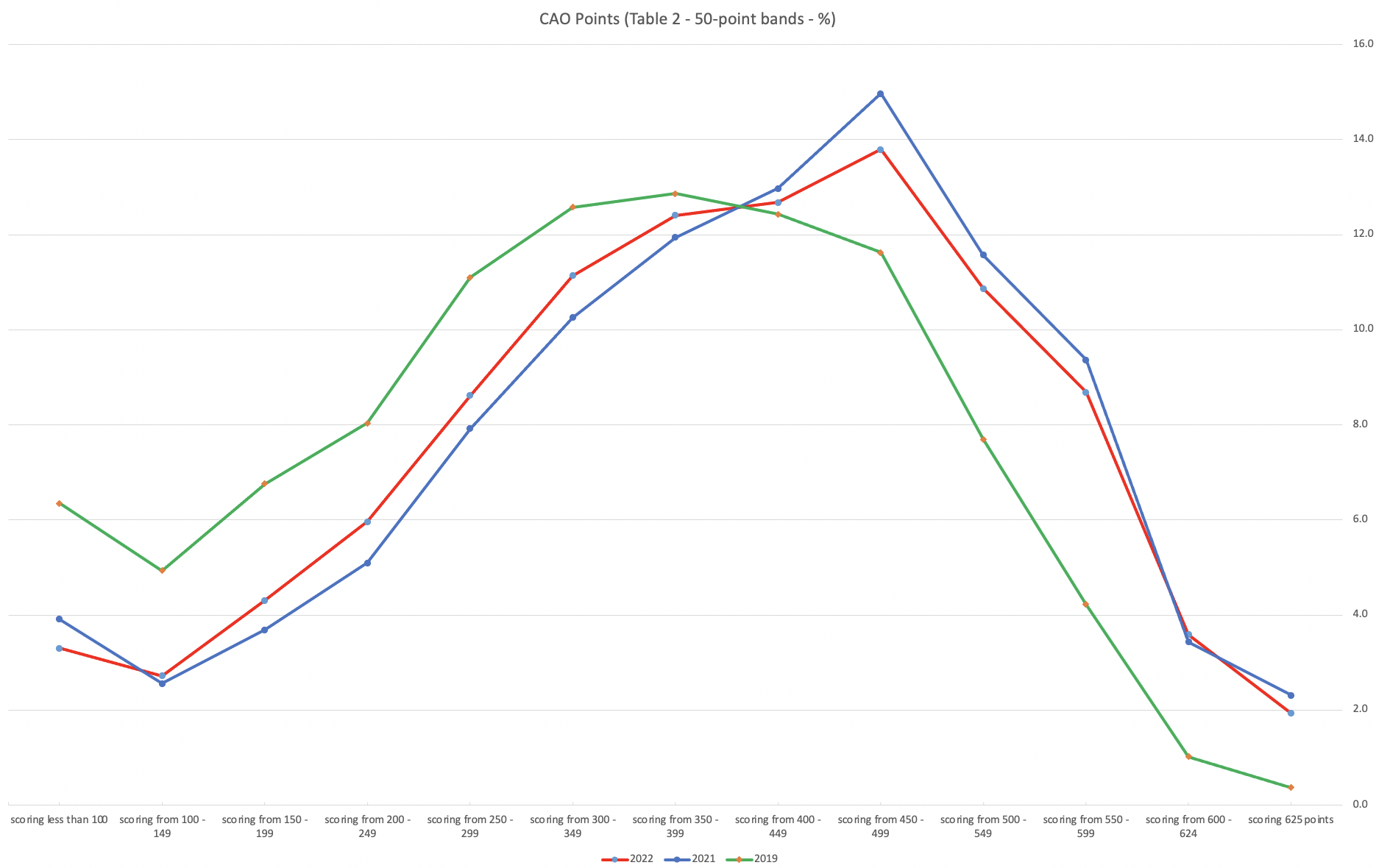
This chart clearly shows a shifting of the profile to the left for the red line which represents 2022. This also supports my blog post last week, and that the Dept of Education has started the process of deflating marks.
Based on this shifting/deflating of marks, we could see the grade/CAO Points profiles reverting back to almost 2019 profile by 2025. For students sitting the Leaving Cert in 2023, there will be another shift to the left, and with another similar shift in 2024. In 2024, the students will be the last group to sit the Leaving Cert who were badly affected during the Covid years. Many of them lost large chunks on school and many didn’t sit the Junior Cert. I’d predict 2025 will see the first time the marks/points profiles will match pre-covid years.
For this analysis I’ve used a variety of tools including Excel, Python and Oracle Analytics.
The Dataset used can be found under Dataset menu, and listed as ‘CAO Points Profiles 2015-2022’. Also, check out the Leaving Certificate 2015-2022 dataset.
Leaving Cert 2022 Results – Inflation, deflation or in-line!
The Leaving Certificate 2022 results are out. Up and down the country there are people who are delighted with their results, while others are disappointed, and lots of other emotions.
The Leaving Certificate is the terminal examination for secondary education in Ireland, with most students being examined in seven subjects, with their best six grades counting towards their “points”, which in turn determines what university course they might get. Check out this link for learn more about the Leaving Certificate.
The Dept of Education has been saying, for several months, this results this year (2022) will be “in-line on aggregate” with the results from 2021. There has been some concerns about grade inflation in 2021 and the impact it will have on the students in 2022 and future years. At some point the Dept of Education needs to address this grade inflation and look to revert back to the normal profile of grades pre-Covid.
Let’s have a look to see if this is true, and if it is true when we look a little deeper. Do the aggregate results hide grade deflation in some subjects.
For the analysis presented in this blog post, I’ve just looked at results at Higher Level across all subjects, and for the deeper dive I’ll look at some of the most popular subjects.
Firstly let’s have a quick look at the distribution of grades by subject for 2022 and 2021.


Remember the Dept of Education said the 2022 results should be in-line with the results of 2021. This required them to apply some adjustments, after marking the exam scripts, to give an updated profile. The following chart shows this comparison between the two years. On initial inspection we can see it is broadly similar. This is good, right? It kind of is and at a high level things look broadly in-line and maybe we can believe the Dept of Education. Looking a little closer we can see a small decrease in the H2-H4 range, and a slight increase in the H5-H8.

Let’s dive a little deeper. When we look at the grade profile of students in 2021 and 2022, How many subjects increased the number of students at each grade vs How many subjects decreased grades vs How many approximately stated the same. The table below shows the results and only counts a change if it is greater than 1% (to allow for minor variations between years).
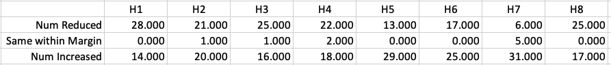
This table in very interesting in that more subjects decreased their H1s, with some variation for the H2-H4s, while for the lower range of H5-H7 we can see there has been an increase in grades. If I increased the margin to 3% we get a slightly different results, but only minor changes.
“in-line on aggregate” might be holding true, although it appears a slight increase on the numbers getting the lower grades. This might indicate either more of an adjustment to weaker students and/or a bit of a down shifting of grades from the H2-H4 range. But at the higher end, more subjects reduced than increase. The overall (aggregate) numbers are potentially masking movements in grade profiles.
Let’s now have a look at some of the core subjects of English, Irish and Mathematics.
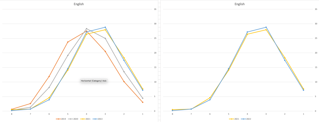
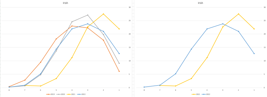

For English, it looks like they fitted to the curve perfectly! keeping grades in-line between the two years. Mathematics is a little different with a slight increase in grades. But when you look at Irish we can see there was definite grade deflation. For each of these subjects, the chart on the left contains four years of data including 2019 when the last “normal” leaving certificate occurred. With Irish the grade profile has been adjusted (deflated) significantly and is closer to 2019 profile than it is to 2021. There was been lots and lots of discussions nationally about how and when grades will revert to normal profile. The 2022 profile for Irish seems to show this has started to happen in this subject, which raises the question if this is occurring in any other subjects, and is hidden/masked by the “in-line on aggregate” figures.
This blog post would become just too long if I was to present the results profile for each of the 42+ subjects.
Let’s have a look as two of the most common foreign languages, French and Spanish.
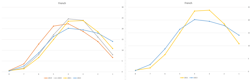
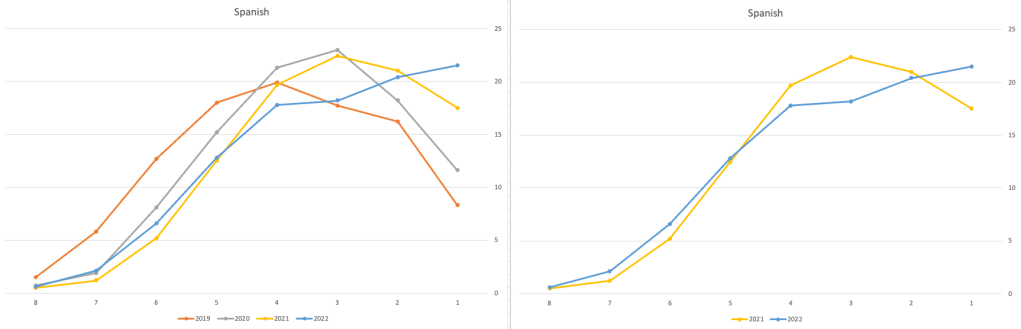
Again we can see some grade deflation, although not to be same extent as Irish. For both French and Spanish, we have reduced numbers for the H2-H4 range and a slight increase for H5-H7, and shift to the left in the profile. A slight exception is for those getting a H1 for both subjects. The adjustment in the results profile is more pronounced for French, and could indicate some deflation adjustments.
Next we’ll look at some of the science subjects of Physics, Chemistry and Biology.
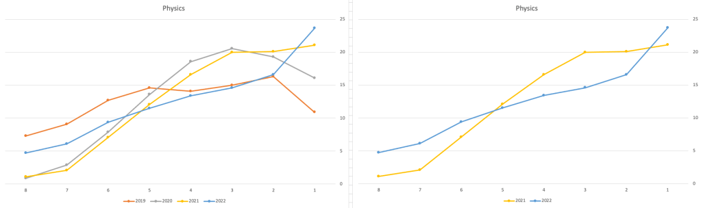
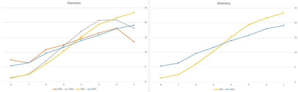
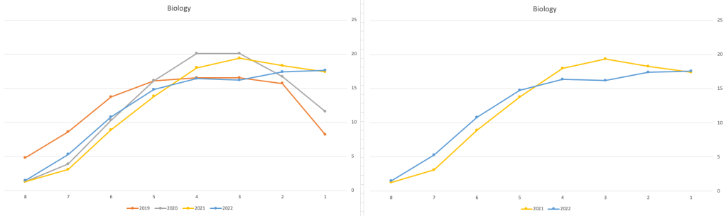
These three subjects also indicate some adjusts back towards the pre-Covid profile, with exception of H1 grades. We can see the 2022 profile almost reflect the 2019 profile (excluding H1s) and for Biology appears to be at a half way point between 2019 and 2022 (excluding H1s)
Just one more example of grade deflation, and this with Design, Communication and Graphics (or DCG)
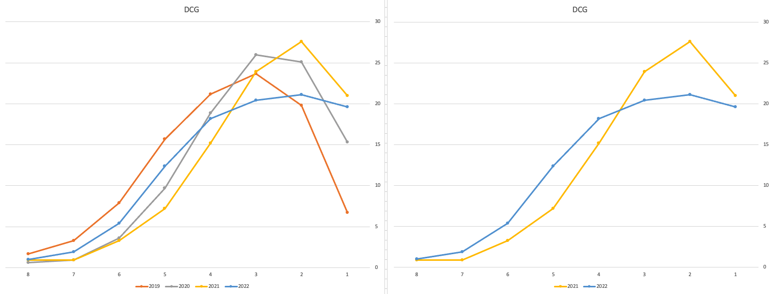
Yes there is obvious grade deflation and almost back to 2019 profile, with the exception of H1s again.
I’ve mentioned some possible grade deflation in various subjects, but there are also subjects where the profile very closely matches the 2021 profile. We have seen above English is one of those. Others include Technology, Art and Computer Science.
I’ve analyzed many more subjects and similar shifting of the profile is evident in those. Has the Dept of Education and State Examinations Commission taken steps to start deflating grades from the highs of 2021? I’d said the answer lies in the data, and the data I’ve looked at shows they have started the deflation process. This might take another couple of years to work out of the system and we will be back to “normal” pre-covid profiles. Which raises another interesting question, Was the grade profile for subjects, pre-covid, fitted to the curve? For the core set of subjects and for many of the more popular subjects, the data seems to indicate this. Maybe the “normal” distribution of marks is down to the “normal” distribution of abilities of the student population each year, or have grades been normalised in some way each year, for years, even decades?
For this analysis I’ve used a variety of tools including Excel, Python and Oracle Analytics.
The Dataset used can be found under Dataset menu, and listed as ‘Leaving Certificate 2015-2022’. An additional Dataset, I’ll be adding soon, will be for CAO Points Profiles 2015-2022.
oracledb Python Library – Connect to DB & a few other changes
Oracle have released a new Python library for connecting to Oracle Databases on-premises and on the Cloud. It’s called (very imaginatively, yet very clearly) oracledb. This new Python library replaces the previous library called cx_Oracle. Just consider cx_oracle as obsolete, and use oracledb going forward, as all development work on new features and enhancements will be done to oracledb.
cx_oracle has been around a long time, and it’s about time we have a new and enhanced library that is more flexible and will suit many different deployment scenarios. The previous library (cx_Oracle) was great, but it did require additional software installation with Oracle Client, and some OS environment settings, which at times took a bit of debugging. This makes it difficult/challenging to deploy in different environments, for example IOTs, CI/CD, containers, etc. Deployment environments have changed and the new oracledb library makes it simpler.
To check out the following links for a full list of new features and other details.
Home page: oracle.github.io/python-oracledb
Installation instructions: python-oracledb.readthedocs.io/en/latest/installation.html
Documentation: python-oracledb.readthedocs.io
One of the main differences between the two libraries is how you connect to the Database. With oracledb you need to use named the parameters, and the new library uses a thin connection. If you need the thick connection you can switch to that easily enough.
The following examples will illustrate how to connect to Oracle Database (local and cloud ADW/ATP) and how these are different to using the cx_Oracle library (which needed Oracle Client software installed). Remember the new oracledb library does not need Oracle Client.
To get started, install oracledb.
pip3 install oracledbLocal Database (running in Docker)
To test connection to a local Database I’m using a Docker image of 21c (hence localhost in this example, replace with IP address for your database). Using the previous library (cx_Oracle) you could concatenate the connection details to form a string and pass that to the connection. With oracledb, you need to use named parameters and specify each part of the connection separately.
This example illustrates this simple connection and prints out some useful information about the connection, do we have a healthy connection, are we using thing database connection and what version is the connection library.
p_username = "..."
p_password = "..."
p_dns = "localhost/XEPDB1"
p_port = "1521"

con = oracledb.connect(user=p_username, password=p_password, dsn=p_dns, port=p_port)

print(con.is_healthy())
print(con.thin)
print(con.version)
---

True
True
21.3.0.0.0
Having created the connection we can now query the Database and close the connection.
cur = con.cursor()
cur.execute('select table_name from user_tables')

for row in cur:
      print(row)

---
('WHISKIES_DATASET',)
('HOLIDAY',)
('STAGE',)
('DIRECTIONS',)
---

cur.close()
con.close()
The code I’ve given above is simple and straight forward. And if you are converting from cx_Oracle, you will probably have minimal changes as you probably had your parameter keywords defined in your code. If not, some simple editing is needed.
To simplify the above code even more, the following does all the same steps without the explicit open and close statements, as these are implicit in this example.
import oracledb

con = oracledb.connect(user=p_username, password=p_password, dsn=p_dns, port=p_port)
with con.cursor() as cursor:
  for row in cursor.execute('select table_name from user_tables'):
      print(row)
(Basic) Oracle Cloud – Autonomous Database, ATP/ADW
Everyone is using the Cloud, Right? If you believe the marketing they are, but in reality most will be working in some hybrid world using a mixture of on-premises and cloud storage. The example given in the previous section illustrated connecting to a local/on-premises database. Let’s now look at connecting to a database on Oracle Cloud (Autonomous Database, ATP/ADW).
With the oracledb library things have been simplified a little. In this section I’ll illustrate a simple connection to a ATP/ADW using a thin connection.
What you need is the location of the directory containing the unzipped wallet file. No Oracle client is needed. If you haven’t downloaded a Wallet file in a while, you should go download a new version of it. The Wallet will contain a pem file which is needed to securely connect to the DB. You’ll also need the password for the Wallet, so talk nicely with your DBA. When setting up the connection you need to provide the directory for the tnsnames.ora file and the ewallet.pem file. If you have downloaded and unzipped the Wallet, these will be in the same directory
import oracledb

p_username = "..."
p_password = "..."

p_walletpass = '...'

#This time we specify the location of the wallet
con = oracledb.connect(user=p_username, password=p_password, dsn="student_high",
                       config_dir="/Users/brendan.tierney/Dropbox/5-Database-Wallets/Wallet_student-Full",
                       wallet_location="/Users/brendan.tierney/Dropbox/5-Database-Wallets/Wallet_student-Full",
                       wallet_password=p_walletpass)

print(con)
con.close()
This method allows you to easily connect to any Oracle Cloud Database.
(Thick Connection) Oracle Cloud – Autonomous Database, ATP/ADW
If you have Oracle Client already installed and set up, and you want to use a thick connection, you will need to initialize the function init_oracle_client.
import oracledb

p_username = "..."
p_password = "..."

#point to directory containing tnsnames.ora
oracledb.init_oracle_client(config_dir="/Applications/instantclient_19_8/network/admin")

con = oracledb.connect(user=p_username, password=p_password, dsn="student_high")

print(con)

con.close()
Warning: Some care is needed with using init_oracle_client. If you use it once in your Python code or App then all connections will use it. You might need to do a code review to look at when this is needed and if not remove all occurrences of it from your Python code.
(Additional Security) Oracle Cloud – Autonomous Database, ATP/ADW
There are a few other additional ways of connecting to a database, but one of my favorite ways to connect involves some additional security, particularly when working with IOT devices, or in scenarios that additional security is needed. Two of these involve using One-way TLS and Mututal TLS connections. The following gives an example of setting up One-Way TLS. This involves setting up the Database to only received data and connections from one particular device via an IP address. This requires you to know the IP address of the device you are using and running the code to connect to the ATP/ADW Database.
To set this up, go to the ATP/ADW details in Oracle Cloud, edit the Access Control List, add the IP address of the client device, disable mutual TLS and download the DB Connection. The following code gives and example of setting up a connection
import oracledb

p_username = "..."
p_password = "..."

adw_dsn = '''(description= (retry_count=20)(retry_delay=3)(address=(protocol=tcps)(port=1522)
             (host=adb.us-ashburn-1.oraclecloud.com))(connect_data=(service_name=a8rk428ojzuffy_student_high.adb.oraclecloud.com))
             (security=(ssl_server_cert_dn="CN=adwc.uscom-east-1.oraclecloud.com,OU=Oracle BMCS US,O=Oracle Corporation,L=Redwood City,ST=California,C=US")))'''

con4 = oracledb.connect(user=p_username, password=p_password, dsn=adw_dsn)
This sets up a secure connection between the client device and the Database.
From my initial testing of existing code/applications (although no formal test cases) it does appear the new oracledb library is processing the queries and data quicker than cx_Oracle. This is good and hopefully we will see more improvements with speed in later releases.
Also don’t forget the impact of changing the buffer size for your database connection. This can have a dramatic effect on speeding up your database interactions. Check out this post which illustrates this.
- ← Previous
- 1
- 2
- 3
- 4
- Next →

You must be logged in to post a comment.