
Data Science
Setting up Julia to work with Oracle Database
For Data Science projects the top three languages every data scientist and machine learning practitioner knows are Python, R and SQL. The ranking or order of importance of these is of some debate and the reason answer is, ‘It Depends’. But one thing is for sure no matter what your environment, SQL skills will be needed, because that’s where the data lives, in the various databases of the organization. No matter what the database is SQL is the way to access and analyze it efficiently. But for Python and R, the popularity of these languages really depends on the project team and their background. Deciding between the two can come down to flipping a coin. But every has their favorite!
A (or not so) new language for data science and machine learning is Julia. Actually it has been around for a while now, and life began on it in 2009, whereas R (and S) and Python have their beginnings back in the 1980’s and early 1990’s. Does that make them legacy programming languages? or it just took a bit of time to mature and gain popularity?
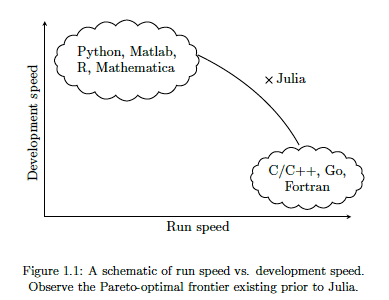
There are lots of advantages to Julia, just like there are lots of advantages with the other languages. The following diagram illustrates one of the core advantages of Julia, it isn’t an interpreted language like R and Python, which means Julia will be significantly faster, yet still allows interactive development using Notebooks, just like R and Python. Julia was designed and build for data science and machine learning, and is designed for scale which makes it a good fit for MLOps. The list of advantages and differences can go on a bit and those are not the point of this post.
The remainder of this post will step through what is needed to get Julia working with an Oracle Database, and you have setup an IDE. Check out the Julia website for excellent installation instructions and selecting an IDE. If you coming from an R and/or Python background, using Jupyter Notebooks is a good option, and as you become more experienced there are a number of more advanced IDEs available for you to use. I’m assuming you have installed Julia.
If you have done a new install of Julia, make sure to add the install directory to the search PATH.
First Download load and install Oracle Instant Client. This is needed by the Julia packages to communicate with Oracle Database. After installing make sure to setup the following in your environment (environment variables and Path)
- ORACLE_HOME : points to where you installed Oracle Instant Client
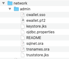
- TNS_ADMIN : points to the directory containing the wallet/tnsnames files. This will be a sub-directory in Oracle Instant Client directory, for example, it points to …/instantclient_19_8/network/admin
- PATH : include the Oracle Instant Client install directory in the PATH.
Next step is to setup the Oracle Client network files. As your DBA for the tnsnames.ora file or for the Wallet Zip file for your database. The Wallet Zip file is the most common approach. Unzip this Wallet file and copy the unzipped files to the TNS_ADMIN directory. See the second bullet point above to for this (…/instantclient_19_8/network/admin).
That’s all you need to do on the Oracle setup. I’m assuming you have a username and password for the Oracle Database you will be using.
Now we can setup Julia to use the Oracle Instant Client software. It is important you have setup those environment variables l’ve listed above.
There is an Oracle.jl package, developed by Felipe Noronha, which runs on top of Oracle Instant Client. To install this, load the Pkg package then then add the Oracle package. The following shows these commands and part of the output from the installation.
julia> using Pkg

julia> Pkg.add("Oracle")
Updating registry at `~/.julia/registries/General`
######################################################################## 100.0%
Resolving package versions...
Installed Reexport ──────────────────── v1.0.0
Installed libsodium_jll ─────────────── v1.0.18+1
Installed Compat ────────────────────── v3.25.0
Installed OrderedCollections ────────── v1.3.3
Installed WebSockets ────────────────── v1.5.9
Installed JuliaInterpreter ──────────── v0.8.8
Installed DataStructures ────────────── v0.18.9
Installed DataAPI ───────────────────── v1.5.1
Installed Requires ──────────────────── v1.1.2
Installed DataValueInterfaces ───────── v1.0.0
Installed Parsers ───────────────────── v1.0.15
Installed FlameGraphs ───────────────── v0.2.5
Installed URIs ──────────────────────── v1.2.0
Installed Colors ────────────────────── v0.12.6
Installed Oracle ────────────────────── v0.2.0
...
...
...
[7240a794] + Oracle v0.2.0
[bac558e1] ↑ OrderedCollections v1.3.2 ⇒ v1.3.3
[69de0a69] ↑ Parsers v1.0.12 ⇒ v1.0.15
[189a3867] ↑ Reexport v0.2.0 ⇒ v1.0.0
[ae029012] ↑ Requires v1.1.1 ⇒ v1.1.2
[3783bdb8] + TableTraits v1.0.0
[bd369af6] + Tables v1.3.2
[0796e94c] ↑ Tokenize v0.5.8 ⇒ v0.5.13
[5c2747f8] + URIs v1.2.0
[104b5d7c] ↑ WebSockets v1.5.2 ⇒ v1.5.9
[8f1865be] ↑ ZeroMQ_jll v4.3.2+5 ⇒ v4.3.2+6
[a9144af2] + libsodium_jll v1.0.18+1
Building Oracle → `~/.julia/packages/Oracle/CEOWz/deps/build.log`

julia>
You are now ready to load this Oracle package and use it to connect to an Oracle Database. Setting up a connection is really simple and in the following example I’m connecting to an ATP Database on Oracle Free Tier. The following sets up some variables, creates a connection, prints a statement and connection information and then closes the connection.
import Oracle

username="oml_user"
password="xxxxxxxxxxx"
dbname="yyyyyyyyyyyy"

conn = Oracle.Connection(username, password, dbname)

println("Connected")
println(conn)

Oracle.close(conn)
Job done 🙂
There is little additional connection information available. To test the connection a bit more let’s list what tables I have in my test/demo schema/user.
import Oracle

username="oml_user"
password="xxxxxxxxxxx"
dbname="yyyyyyyyyyyy"

conn = Oracle.Connection(username, password, dbname)

println("Tables")
println("--------------------")

Oracle.query(conn, "SELECT table_name FROM user_tables") do cursor
    for row in cursor
    # row values can be accessed using column name or position
        println( row["TABLE_NAME"] ) # same as row[1]
    end
end

println("")
println("...the end...")

Oracle.close(conn)
If you come from a Python background the syntax is familiar which makes the move other to Julia an easier task.
One other difference is, running the above code does seem to run a lot quicker in Julia. I haven’t measured it and the difference is less than a second but it is noticeable. For me, the above code generate the following output,
Tables
--------------------
WINE
BANK_ADDITIONAL_FULL
MINING_DATA_BUILD_V

...the end...
I’ll have additional posts looking are difference aspects and commands for working with and processing data in an Oracle Database.
2020 Books on Data Science and Machine Learning
2020 has been an interesting year. Not for the obvious topic, but for new books on Data Science and Machine Learning. The list below are some of my favorite books from 2020. Making the selection was difficult. Some months had a large number of releases and some were a bit quieter. The books below are listed based on their release date and are not ranked in any way. I’ve included links to these books on Amazon (.com, .uk and .de).
 |
 |
 |
|
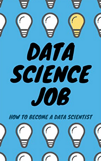
| January
Everyone wants to work in Data Science, but where and how do you start. Aimed at beginners with guidance without the technical. High level, not for everyone. |
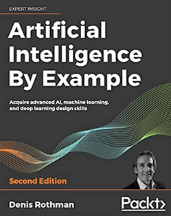
February
Taking ML to the next stage creating AI application. How to do it with examples across a number of areas. |
March
A guide for those wary of impact of technology’s and for those who are enthusiastic about where AI is taking us. |
|
 |
 |
 |
|
| April
AI Ethics was one of the topic topics for 2020. Covers the philosophical aspects along with the technical one.s |
May
Covering the life-cyle of building ML application, showing all that it entails and how ML plays a small part in the overall solution |
June
From covering the basics of NLP, it builds on this to include in application, how to use in different industries and within project teams. |
|
 |
 |
 |
|
| July
With by Thomas Davenport and others, and is a good addition to his other books. Consisting of interviews, research and analysis on how to win with ML & AI. |
August
I was invited to contribute a couple of chapters to this book, along with well known names in areas of DS, ML & AI |
September
Building upon the success of their 1st edition, the 2nd edition comes with more example and extra chapters. |
|
 |
 |
 |
|
| October
ML & AI is not perfect. Lots can go wrong. Not just with the project but also with the implementation of the applications. Lots to thing about and consider. |
November
No one really builds ML algorithms. We build ML solutions and applications. But whats the best way to do this, from technical, organizational and ethical aspects. |
December
It was difficult to pick a book for this month. Lots of new releases and I haven’t received all my orders, at time of this post. Here is a book from July, and is related to an Automated Trading App I’ve been working on (and earning) for a couple of years. |
And to finish off the list I’m including this additional book. It wasn’t released this year. It was released in April 2018. It was a best seller on Amazon in 2018 and 2019! This was really exciting for us and we still amazed at how it it is still selling in 2020. It is currently, as of December 2020, listed in 8th place on the MIT Press Best Sellers list. It won’t be making any best seller list in 2020, but is still proving popular with many readers. To all of you who have bought this book, I’d like to say Thank You and wishing you all the best with 2021 and beyond.
Adding Text Processing to Classification Machine Learning in Oracle Machine Learning
One of the typical machine learning functions is Classification. This is in widespread use across most domains and geographic regions. I’ve written several blog posts on this topic over many years (and going back many, many year) on how to do this using Oracle Machine Learning (OML) (formally known as Oracle Advanced Analytic and in the Oracle Data Miner tool in SQL Developer). Just do a quick search of my blog to find some of these posts.
When it comes to Classification problems, typically the data set will be contain your typical categorical and numerical variables/features. The Automatic Data Preparation (ADP) feature of OML where it automatically pre-processes and transforms these variable for input to the machine learning algorithm. This greatly reduces the boring work of the data scientist and increases their productivity.
But sometimes data sets come with text descriptions. These will contain production descriptions, free format text, and other descriptive data, for example product reviews. But how can this information be included as part of the input data set to the machine learning algorithms. Oracle allows this kind of input data, and a letting bit of setup is needed to tell Oracle how to process the data set. This uses the in-database feature of Oracle Text.
The following example walks through an example of the steps needed to pre-process and include the text processing as part of the machine learning algorithm.
The data set: The data used to illustrate this and to show the steps needed, is a data set from Kaggle webiste. This data set contains 130K Wine Reviews. This data set contain descriptive information of the wine with attributes about each wine including country, region, number of points, price, etc as well as a text description contain a review of the wine.
The following are 2 files containing the DDL (to create the table) and then Import the data set (using sql script with insert statements). These can be run in your schema (in order listed below).
I’ll leave the Data Exploration to you to do and to discover some early insights.
The ML Question
I want to be able to predict if a wine is a good quality wine, based on the prices and different characteristics of the wine?
Data Preparation
To be able to answer this question the first thing needed is to define a target variable to identify good and bad wines. To do this create a new attribute/feature called POINTS_BIN and populate it based on the number of points a wine has. If it has >90 points it is a good wine, if <90 points it is a bad wine.
ALTER TABLE WineReviews130K_bin ADD POINTS_BIN VARCHAR2(15);

UPDATE WineReviews130K_bin
SET POINTS_BIN = 'GT_90_Points'
WHERE winereviews130k_bin.POINTS >= 90;

UPDATE WineReviews130K_bin
SET POINTS_BIN = 'LT_90_Points'
WHERE winereviews130k_bin.POINTS < 90;

alter table WineReviews130K_bin DROP COLUMN POINTS;
The DESCRIPTION column data type needs to be changed to CLOB. This is to allow the Text Mining feature to work correctly.
-- add a new column of data type CLOB
ALTER TABLE WineReviews130K_bin ADD (DESCRIPTION_NEW CLOB);

-- update new column with data from the DESCRIPTION attribute
UPDATE WineReviews130K_bin SET DESCRIPTION_NEW = DESCRIPTION;

-- drop the DESCRIPTION attribute from table
ALTER TABLE WineReviews130K_bin DROP COLUMN DESCRIPTION;

-- rename the new attribute to replace DESCRIPTION
ALTER TABLE WineReviews130K_bin RENAME COLUMN DESCRIPTION_NEW TO DESCRIPTION;
Text Mining Configuration
There are a number of things we need to define for the Text Mining to work, these include a Lexer, Stop Word list and preferences.
First define the Lexer to use. In this case we will use a basic one and basic settings
BEGIN
   ctx_ddl.create_preference('mylex', 'BASIC_LEXER');
   ctx_ddl.set_attribute('mylex', 'printjoins', '_-');
   ctx_ddl.set_attribute ( 'mylex', 'index_themes', 'NO');
   ctx_ddl.set_attribute ( 'mylex', 'index_text', 'YES');
END;
Next we can define a Stop Word List. Oracle Text comes with a predefined set of Stop Word lists for most of the common languages. You can add to one of those list or create your own. Depending on the domain you are working in it might be easier to create your own and it is very straight forward to do. For example:
DECLARE
   v_stoplist_name varchar2(100);
BEGIN
   v_stoplist_name := 'mystop';
   ctx_ddl.create_stoplist(v_stoplist_name, 'BASIC_STOPLIST');
   ctx_ddl.add_stopword(v_stoplist_name, 'nonetheless');
   ctx_ddl.add_stopword(v_stoplist_name, 'Mr');
   ctx_ddl.add_stopword(v_stoplist_name, 'Mrs');
   ctx_ddl.add_stopword(v_stoplist_name, 'Ms');
   ctx_ddl.add_stopword(v_stoplist_name, 'a');
   ctx_ddl.add_stopword(v_stoplist_name, 'all');
   ctx_ddl.add_stopword(v_stoplist_name, 'almost');
   ctx_ddl.add_stopword(v_stoplist_name, 'also');
   ctx_ddl.add_stopword(v_stoplist_name, 'although');
   ctx_ddl.add_stopword(v_stoplist_name, 'an');
   ctx_ddl.add_stopword(v_stoplist_name, 'and');
   ctx_ddl.add_stopword(v_stoplist_name, 'any');
   ctx_ddl.add_stopword(v_stoplist_name, 'are');
   ctx_ddl.add_stopword(v_stoplist_name, 'as');
   ctx_ddl.add_stopword(v_stoplist_name, 'at');
   ctx_ddl.add_stopword(v_stoplist_name, 'be');
   ctx_ddl.add_stopword(v_stoplist_name, 'because');
   ctx_ddl.add_stopword(v_stoplist_name, 'been');
   ctx_ddl.add_stopword(v_stoplist_name, 'both');
   ctx_ddl.add_stopword(v_stoplist_name, 'but');
   ctx_ddl.add_stopword(v_stoplist_name, 'by');
   ctx_ddl.add_stopword(v_stoplist_name, 'can');
   ctx_ddl.add_stopword(v_stoplist_name, 'could');
   ctx_ddl.add_stopword(v_stoplist_name, 'd');
   ctx_ddl.add_stopword(v_stoplist_name, 'did');
   ctx_ddl.add_stopword(v_stoplist_name, 'do');
   ctx_ddl.add_stopword(v_stoplist_name, 'does');
   ctx_ddl.add_stopword(v_stoplist_name, 'either');
   ctx_ddl.add_stopword(v_stoplist_name, 'for');
   ctx_ddl.add_stopword(v_stoplist_name, 'from');
   ctx_ddl.add_stopword(v_stoplist_name, 'had');
   ctx_ddl.add_stopword(v_stoplist_name, 'has');
   ctx_ddl.add_stopword(v_stoplist_name, 'have');
   ctx_ddl.add_stopword(v_stoplist_name, 'having');
   ctx_ddl.add_stopword(v_stoplist_name, 'he');
   ctx_ddl.add_stopword(v_stoplist_name, 'her');
   ctx_ddl.add_stopword(v_stoplist_name, 'here');
   ctx_ddl.add_stopword(v_stoplist_name, 'hers');
   ctx_ddl.add_stopword(v_stoplist_name, 'him');
   ctx_ddl.add_stopword(v_stoplist_name, 'his');
   ctx_ddl.add_stopword(v_stoplist_name, 'how');
   ctx_ddl.add_stopword(v_stoplist_name, 'however');
   ctx_ddl.add_stopword(v_stoplist_name, 'i');
   ctx_ddl.add_stopword(v_stoplist_name, 'if');
   ctx_ddl.add_stopword(v_stoplist_name, 'in');
   ctx_ddl.add_stopword(v_stoplist_name, 'into');
   ctx_ddl.add_stopword(v_stoplist_name, 'is');
   ctx_ddl.add_stopword(v_stoplist_name, 'it');
   ctx_ddl.add_stopword(v_stoplist_name, 'its');
   ctx_ddl.add_stopword(v_stoplist_name, 'just');
   ctx_ddl.add_stopword(v_stoplist_name, 'll');
   ctx_ddl.add_stopword(v_stoplist_name, 'me');
   ctx_ddl.add_stopword(v_stoplist_name, 'might');
   ctx_ddl.add_stopword(v_stoplist_name, 'my');
   ctx_ddl.add_stopword(v_stoplist_name, 'no');
   ctx_ddl.add_stopword(v_stoplist_name, 'non');
   ctx_ddl.add_stopword(v_stoplist_name, 'nor');
   ctx_ddl.add_stopword(v_stoplist_name, 'not');
   ctx_ddl.add_stopword(v_stoplist_name, 'of');
   ctx_ddl.add_stopword(v_stoplist_name, 'on');
   ctx_ddl.add_stopword(v_stoplist_name, 'one');
   ctx_ddl.add_stopword(v_stoplist_name, 'only');
   ctx_ddl.add_stopword(v_stoplist_name, 'onto');
   ctx_ddl.add_stopword(v_stoplist_name, 'or');
   ctx_ddl.add_stopword(v_stoplist_name, 'our');
   ctx_ddl.add_stopword(v_stoplist_name, 'ours');
   ctx_ddl.add_stopword(v_stoplist_name, 's');
   ctx_ddl.add_stopword(v_stoplist_name, 'shall');
   ctx_ddl.add_stopword(v_stoplist_name, 'she');
   ctx_ddl.add_stopword(v_stoplist_name, 'should');
   ctx_ddl.add_stopword(v_stoplist_name, 'since');
   ctx_ddl.add_stopword(v_stoplist_name, 'so');
   ctx_ddl.add_stopword(v_stoplist_name, 'some');
   ctx_ddl.add_stopword(v_stoplist_name, 'still');
   ctx_ddl.add_stopword(v_stoplist_name, 'such');
   ctx_ddl.add_stopword(v_stoplist_name, 't');
   ctx_ddl.add_stopword(v_stoplist_name, 'than');
   ctx_ddl.add_stopword(v_stoplist_name, 'that');
   ctx_ddl.add_stopword(v_stoplist_name, 'the');
   ctx_ddl.add_stopword(v_stoplist_name, 'their');
   ctx_ddl.add_stopword(v_stoplist_name, 'them');
   ctx_ddl.add_stopword(v_stoplist_name, 'then');
   ctx_ddl.add_stopword(v_stoplist_name, 'there');
   ctx_ddl.add_stopword(v_stoplist_name, 'therefore');
   ctx_ddl.add_stopword(v_stoplist_name, 'these');
   ctx_ddl.add_stopword(v_stoplist_name, 'they');
   ctx_ddl.add_stopword(v_stoplist_name, 'this');
   ctx_ddl.add_stopword(v_stoplist_name, 'those');
   ctx_ddl.add_stopword(v_stoplist_name, 'though');
   ctx_ddl.add_stopword(v_stoplist_name, 'through');
   ctx_ddl.add_stopword(v_stoplist_name, 'thus');
   ctx_ddl.add_stopword(v_stoplist_name, 'to');
   ctx_ddl.add_stopword(v_stoplist_name, 'too');
   ctx_ddl.add_stopword(v_stoplist_name, 'until');
   ctx_ddl.add_stopword(v_stoplist_name, 've');
   ctx_ddl.add_stopword(v_stoplist_name, 'very');
   ctx_ddl.add_stopword(v_stoplist_name, 'was');
   ctx_ddl.add_stopword(v_stoplist_name, 'we');
   ctx_ddl.add_stopword(v_stoplist_name, 'were');
   ctx_ddl.add_stopword(v_stoplist_name, 'what');
   ctx_ddl.add_stopword(v_stoplist_name, 'when');
   ctx_ddl.add_stopword(v_stoplist_name, 'where');
   ctx_ddl.add_stopword(v_stoplist_name, 'whether');
   ctx_ddl.add_stopword(v_stoplist_name, 'which');
   ctx_ddl.add_stopword(v_stoplist_name, 'while');
   ctx_ddl.add_stopword(v_stoplist_name, 'who');
   ctx_ddl.add_stopword(v_stoplist_name, 'whose');
   ctx_ddl.add_stopword(v_stoplist_name, 'why');
   ctx_ddl.add_stopword(v_stoplist_name, 'will');
   ctx_ddl.add_stopword(v_stoplist_name, 'with');
   ctx_ddl.add_stopword(v_stoplist_name, 'would');
   ctx_ddl.add_stopword(v_stoplist_name, 'yet');
   ctx_ddl.add_stopword(v_stoplist_name, 'you');
   ctx_ddl.add_stopword(v_stoplist_name, 'your');
   ctx_ddl.add_stopword(v_stoplist_name, 'yours');
   ctx_ddl.add_stopword(v_stoplist_name, 'drink');
   ctx_ddl.add_stopword(v_stoplist_name, 'flavors');
   ctx_ddl.add_stopword(v_stoplist_name, '2020');
   ctx_ddl.add_stopword(v_stoplist_name, 'now');
END;
Next define the preferences for processing the Text, for example what Stop Word list to use, if Fuzzy match is to be used and what language to use for this, number of tokens/words to process and if stemming is to be used.
BEGIN
   ctx_ddl.create_preference('mywordlist', 'BASIC_WORDLIST');
   ctx_ddl.set_attribute('mywordlist','FUZZY_MATCH','ENGLISH');
   ctx_ddl.set_attribute('mywordlist','FUZZY_SCORE','1');
   ctx_ddl.set_attribute('mywordlist','FUZZY_NUMRESULTS','5000');
   ctx_ddl.set_attribute('mywordlist','SUBSTRING_INDEX','TRUE');
   ctx_ddl.set_attribute('mywordlist','STEMMER','ENGLISH');
END;
And the final step is to piece it all together by defining a new Text policy
BEGIN
   ctx_ddl.create_policy('my_policy', NULL, NULL, 'mylex', 'mystop', 'mywordlist');
END;
Define Settings for OML Model
We will create two models. An Attribute Importance model and a Classification model. The following defines the model parameters for each of these.
CREATE TABLE att_import_model_settings (setting_name varchar2(30), setting_value varchar2(30));
INSERT INTO att_import_model_settings (setting_name, setting_value)
VALUES (''ALGO_NAME'', ''ALGO_AI_MDL'');
INSERT INTO att_import_model_settings (setting_name, setting_value)
VALUES (''PREP_AUTO'', ''ON'');
INSERT INTO att_import_model_settings (setting_name, setting_value)
VALUES (''ODMS_TEXT_POLICY_NAME'', ''my_policy'');
INSERT INTO att_import_model_settings (setting_name, setting_value)
VALUES (''ODMS_TEXT_MAX_FEATURES'', ''3000'')';
CREATE TABLE wine_model_settings (setting_name varchar2(30), setting_value varchar2(30));
INSERT INTO wine_model_settings (setting_name, setting_value)
VALUES (''ALGO_NAME'', ''ALGO_RANDOM_FOREST'');
INSERT INTO wine_model_settings (setting_name, setting_value)
VALUES (''PREP_AUTO'', ''ON'');
INSERT INTO wine_model_settings (setting_name, setting_value)
VALUES (''ODMS_TEXT_POLICY_NAME'', ''my_policy'');
INSERT INTO wine_model_settings (setting_name, setting_value)
VALUES (''ODMS_TEXT_MAX_FEATURES'', ''3000'')';
Create the Training and Test data sets.
CREATE TABLE wine_train_data
AS SELECT id, country, description, designation, points_bin, price, province, region_1, region_2, taster_name, variety, title
FROM winereviews130k_bin
SAMPLE (60) SEED (1);
CREATE TABLE wine_test_data
AS SELECT id, country, description, designation, points_bin, price, province, region_1, region_2, taster_name, variety, title
FROM winereviews130k_bin
WHERE id NOT IN (SELECT id FROM wine_train_data);
All the set up is done, we can move onto the creating the machine learning models.
Create the OML Model (Attribute Importance & Classification)
We are going to create two models. The first is an Attribute Important model. This will look at the data set and will determine what attributes contribute most towards determining the target variable. As we are incorporting Texting Mining we will see what words/tokens from the DESCRIPTION attribute also contribute towards the target variable.
BEGIN
   DBMS_DATA_MINING.CREATE_MODEL(
      model_name          => 'GOOD_WINE_AI',
      mining_function     => DBMS_DATA_MINING.ATTRIBUTE_IMPORTANCE,
      data_table_name     => 'winereviews130k_bin',
      case_id_column_name => 'ID',
      target_column_name  => 'POINTS_BIN',
      settings_table_name => 'att_import_mode_settings');
END;
We can query the system views for Oracle ML to find out what are the important variables.
SELECT * FROM dm$vagood_wine_ai
ORDER BY attribute_rank;
Here is the listing of the top 15 most important attributes. We can see from the first 15 rows and looking under column ATTRIBUTE_SUBNAME, the words from the DESCRIPTION attribute that seem to be important and contribute towards determining the value in the target attribute.

At this point you might determine, based on domain knowledge, some of these words should be excluded as they are generic for the domain. In this case, go back to the Stop Word List and recreate it with any additional words. This can be repeated until you are happy with the list. In this example, WINE could be excluded by including it in the Stop Word List.
Run the following to create the Classification model. It is very similar to what we ran above with minor changes to the name of the model, the data mining function and the name of the settings table.
BEGIN
   DBMS_DATA_MINING.CREATE_MODEL(
      model_name          => 'GOOD_WINE_MODEL',
      mining_function     => DBMS_DATA_MINING.CLASSIFICATION,
      data_table_name     => 'winereviews130k_bin',
      case_id_column_name => 'ID',
      target_column_name  => 'POINTS_BIN',
      settings_table_name => 'wine_model_settings');
END;
Apply OML Model
The model can be applied in similar ways to any other ML model created using OML. For example the following displays the wine details along with the predicted points bin values (good or bad) and the probability score (<=1) of the prediction.
SELECT id, price, country, designation, province, variety, points_bin,
       PREDICTION(good_wine_mode USING *) pred_points_bin,
       PREDICTION_PROBABILITY(good_wine_mode USING *) prob_points_bin
FROM wine_test_data;
Exploring Database trends using Python pytrends (Google Trends)
A little word of warning before you read the rest of this post. The examples shown below are just examples of what is possible. It isn’t very scientific or rigorous, so don’t come complaining if what is shown doesn’t match your knowledge and other insights. This is just a little fun to see what is possible. Yes a more rigorous scientific study is needed, and some attempts at this can be seen at DB-Engines.com. Less scientific are examples shown at TOPDB Top Database index and that isn’t meant to be very scientific.
After all of that, here we go 🙂
pytrends is a library providing an API to Google Trends using Python. The following examples show some ways you can use this library and the focus area I’ll be using is Databases. Many of you are already familiar with using Google Trends, and if this isn’t something you have looked at before then I’d encourage you to go have a look at their website and to give it a try. You don’t need to run Python to use it. For example, here is a quick example taken from the Google Trends website. Here are a couple of screen shots from Google Trends, comparing Relational Database to NoSQL Database. The information presented is based on what searches have been performed over the past 12 months. Some of the information is kind of interesting when you look at the related queries and also the distribution of countries.


To install pytrends use the pip command
pip3 install pytrends
As usual it will change the various pendent libraries and will update where necessary. In my particular case, the only library it updated was the version of pandas.
You do need to be careful of how many searches you perform as you may be limited due to Google rate limits. You can get around this by using a proxy and there is an example on the pytrends PyPi website on how to get around this.
The following code illustrates how to import and setup an initial request. The pandas library is also loaded as the data returned by pytrends API into a pandas dataframe. This will make it ease to format and explore the data.
import pandas as pd
from pytrends.request import TrendReq

pytrends = TrendReq()
The pytrends API has about nine methods. For my example I’ll be using the following:
- Interest Over Time: returns historical, indexed data for when the keyword was searched most as shown on Google Trends’ Interest Over Time section.
- Interest by Region: returns data for where the keyword is most searched as shown on Google Trends’ Interest by Region section.
- Related Queries: returns data for the related keywords to a provided keyword shown on Google Trends’ Related Queries section.
- Suggestions: returns a list of additional suggested keywords that can be used to refine a trend search.
Let’s now explore these APIs using the Databases as the main topic of investigation and examining some of the different products. I’ve used the db-engines.com website to select the top 5 databases (as per date of this blog post). These were:
- Oracle
- MySQL
- SQL Server
- PostgreSQL
- MongoDB
I will use this list to look for number of searches and other related information. First thing is to import the necessary libraries and create the connection to Google Trends.
import pandas as pd
from pytrends.request import TrendReq

pytrends = TrendReq()
Next setup the payload and keep the timeframe for searches to the past 12 months only.
search_list = ["Oracle", "MySQL", "SQL Server", "PostgreSQL", "MongoDB"] #max of 5 values allowed
pytrends.build_payload(search_list, timeframe='today 12-m')
We can now look at the the interest over time method to see the number of searches, based on a ranking where 100 is the most popular.
df_ot = pd.DataFrame(pytrends.interest_over_time()).drop(columns='isPartial')
df_ot

and to see a breakdown of these number on an hourly bases you can use the get_historical_interest method.
pytrends.get_historical_interest(search_list)
Let’s move on to exploring the level of interest/searches by country. The following retrieves this information, ordered by Oracle (in decending order) and then select the top 20 countries. Here we can see the relative number of searches per country. Note these doe not necessarily related to the countries with the largest number of searches
df_ibr = pytrends.interest_by_region(resolution='COUNTRY') # CITY, COUNTRY or REGION
df_ibr.sort_values('Oracle', ascending=False).head(20)

Visualizing data is always a good thing to do as we can see a patterns and differences in the data in a clearer way. The following takes the above query and creates a stacked bar chart.
import matplotlib
from matplotlib import pyplot as plt

df2 = df_ibr.sort_values('Oracle', ascending=False).head(20)

df2.reset_index().plot(x='geoName', y=['Oracle', 'MySQL', 'SQL Server', 'PostgreSQL', 'MongoDB'], kind ='bar', stacked=True, title="Searches by Country")

plt.rcParams["figure.figsize"] = [20, 8]
plt.xlabel("Country")
plt.ylabel("Ranking")

We can delve into the data more, by focusing on one particular country and examine the google searches by city or region. The following looks at the data from USA and gives the rankings for the various states.
pytrends.build_payload(search_list, geo='US')
df_ibr = pytrends.interest_by_region(resolution='COUNTRY', inc_low_vol=True)
df_ibr.sort_values('Oracle', ascending=False).head(20)

df2.reset_index().plot(x='geoName', y=['Oracle', 'MySQL', 'SQL Server', 'PostgreSQL', 'MongoDB'], kind ='bar', stacked=True, title="test")
plt.rcParams["figure.figsize"] = [20, 8]

plt.title("Searches for USA")
plt.xlabel("State")
plt.ylabel("Ranking")


We can find the top related queries and and top queries including the names of each database.
search_list = ["Oracle", "MySQL", "SQL Server", "PostgreSQL", "MongoDB"] #max of 5 values allowed
pytrends.build_payload(search_list, timeframe='today 12-m')

rq = pytrends.related_queries()
rq.values()

#display rising terms
rq.get('Oracle').get('rising')
We can see the top related rising queries for Oracle are about tik tok. No real surprise there!

and the top queries for Oracle included:
rq.get('Oracle').get('top')

This was an interesting exercise to do. I didn’t show all the results, but when you explore the other databases in the list and see the results from those, and then compare them across the five databases you get to see some interesting patterns.
Principal Component Analysis (PCA) in Oracle
Principal Component Analysis (PCA), is a statistical process used for feature or dimensionality reduction in data science and machine learning projects. It summarizes the features of a large data set into a smaller set of features by projecting each data point onto only the first few principal components to obtain lower-dimensional data while preserving as much of the data’s variation as possible. There are lots of resources that goes into the mathematics behind this approach. I’m not going to go into that detail here and a quick internet search will get you what you need.
PCA can be used to discover important features from large data sets (large as in having a large number of features), while preserving as much information as possible.
Oracle has implemented PCA using Sigular Value Decomposition (SVD) on the covariance and correlations between variables, for feature extraction/reduction. PCA is closely related to SVD. PCA computes a set of orthonormal bases (principal components) that are ranked by their corresponding explained variance. The main difference between SVD and PCA is that the PCA projection is not scaled by the singular values. The extracted features are transformed features consisting of linear combinations of the original features.
When machine learning is performed on this reduced set of transformed features, it can completed with less resources and time, while still maintaining accuracy.
Algorithm Name in Oracle using
Mining Model Function = FEATURE_EXTRACTION
Algorithm = ALGO_SINGULAR_VALUE_DECOMP
(Hyper)-Parameters for algorithms
- SVDS_U_MATRIX_OUTPUT : SVDS_U_MATRIX_ENABLE or SVDS_U_MATRIX_DISABLE
- SVDS_SCORING_MODE : SVDS_SCORING_SVD or SVDS_SCORING_PCA
- SVDS_SOLVER : possible values include SVDS_SOLVER_TSSVD, SVDS_SOLVER_TSEIGEN, SVDS_SOLVER_SSVD, SVDS_SOLVER_STEIGEN
- SVDS_TOLERANCE : range of 0…1
- SVDS_RANDOM_SEED : range of 0…4294967296 (!)
- SVDS_OVER_SAMPLING : range of 1…5000
- SVDS_POWER_ITERATIONS : Default value 2, with possible range of 0…20
Let’s work through an example using the MINING_DATA_BUILD_V data set that comes with Oracle Data Miner.
First step is to define the parameter settings for the algorithm. No data preparation is needed as the algorithm takes care of this. This means you can disable the Automatic Data Preparation (ADP).
-- create the parameter table
CREATE TABLE svd_settings (
setting_name VARCHAR2(30),
setting_value VARCHAR2(4000));

-- define the settings for SVD algorithm
BEGIN
   INSERT INTO svd_settings (setting_name, setting_value)
   VALUES (dbms_data_mining.algo_name, dbms_data_mining.algo_singular_value_decomp);

   -- turn OFF ADP
   INSERT INTO svd_settings (setting_name, setting_value)
   VALUES (dbms_data_mining.prep_auto, dbms_data_mining.prep_auto_off);

   -- set PCA scoring mode
   INSERT INTO svd_settings (setting_name, setting_value)
   VALUES (dbms_data_mining.svds_scoring_mode, dbms_data_mining.svds_scoring_pca);

   INSERT INTO svd_settings (setting_name, setting_value)
   VALUES (dbms_data_mining.prep_shift_2dnum, dbms_data_mining.prep_shift_mean);

   INSERT INTO svd_settings (setting_name, setting_value)
   VALUES (dbms_data_mining.prep_scale_2dnum, dbms_data_mining.prep_scale_stddev);
END;
/
You are now ready to create the model.
BEGIN
   DBMS_DATA_MINING.CREATE_MODEL(
      model_name          => 'SVD_MODEL',
      mining_function     => dbms_data_mining.feature_extraction,
      data_table_name     => 'mining_data_build_v',
      case_id_column_name => 'CUST_ID',
      settings_table_name => 'svd_settings');
END;
When created you can use the mining model data dictionary views to explore the model and to explore the specifics of the model and the various MxN matrix created using the model specific views. These include:
- DM$VESVD_Model : Singular Value Decomposition S Matrix
- DM$VGSVD_Model : Global Name-Value Pairs
- DM$VNSVD_Model : Normalization and Missing Value Handling
- DM$VSSVD_Model : Computed Settings
- DM$VUSVD_Model : Singular Value Decomposition U Matrix
- DM$VVSVD_Model : Singular Value Decomposition V Matrix
- DM$VWSVD_Model : Model Build Alerts
Where the S, V and U matrix contain:
- U matrix : consists of a set of ‘left’ orthonormal bases
- S matrix : is a diagonal matrix
- V matrix : consists of set of ‘right’ orthonormal bases
These can be explored using the following
-- S matrix
select feature_id, VALUE, variance, pct_cum_variance
from DM$VESVD_MODEL;

-- V matrix
select feature_id, attribute_name, value
from DM$VVSVD_MODEL
order by feature_id, attribute_name;

-- U matrix
select feature_id, attribute_name, value
from DM$VVSVD_MODEL
order by feature_id, attribute_name;
To determine the projections to be used for visualizations we can use the FEATURE_VALUES function.
select FEATURE_VALUE(svd_sh_sample, 1 USING *) proj1,
       FEATURE_VALUE(svd_sh_sample, 2 USING *) proj2
from   mining_data_build_v
where  cust_id <= 101510
order by 1, 2;
Other algorithms available in Oracle for feature extraction and reduction include:
- Non-Negative Matrix Factorization (NMF)
- Explicit Semantic Analysis (ESA)
- Minimum Description Length (MDL) – this is really feature selection rather than feature extraction
OCI Data Science – Create a Project & Notebook, and Explore the Interface
In my previous blog post I went through the steps of setting up OCI to allow you to access OCI Data Science. Those steps showed the setup and configuration for your Data Science Team.

In this post I will walk through the steps necessary to create an OCI Data Science Project and Notebook, and will then Explore the basic Notebook environment.
1 – Create a Project
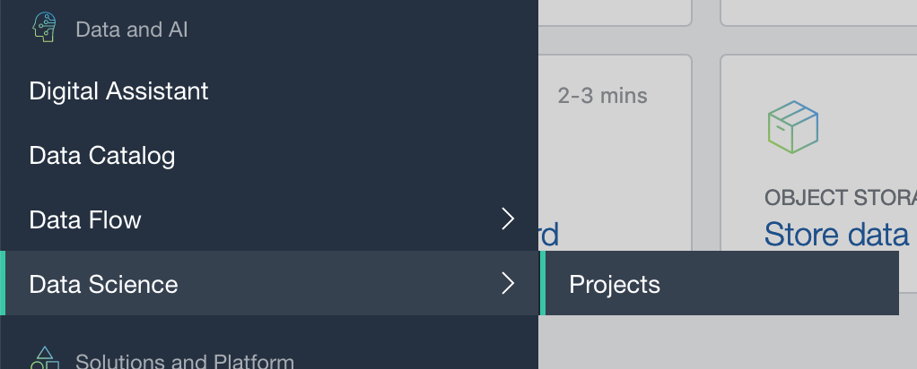
From the main menu on the Oracle Cloud home page select Data Science -> Projects from the menu.
Select the appropriate Compartment in the drop-down list on the left hand side of the screen. In my previous blog post I created a separate Compartment for my Data Science work and team. Then click on the Create Projects button.
 Enter a name for your project. I called this project, ‘DS-Demo-Project’. Click Create button.
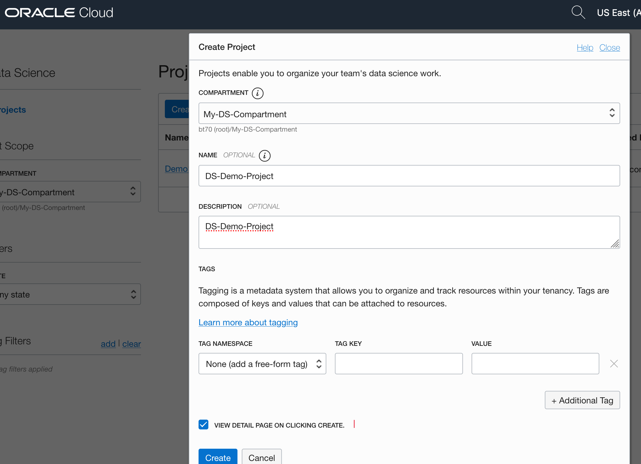

That’s the Project created.
2 – Create a Notebook
After creating a project (see above) you can not create one or many Notebook Sessions.
To create a Notebook Session click on the Create Notebook Session button (see the above image). This will create a VM to contain your notebook and associated work. Just like all VM in Oracle Cloud, they come in various different shapes. These can be adjusted at a later time to scale up and then back down based on the work you will be performing.
The following example creates a Notebook Session using the basic VM shape. I call the Notebook ‘DS-Demo-Notebook’. I also set the Block Storage size to 50G, which is the minimum value. The VNC details have been defaulted to those assigned to the Compartment. Click Create button at the bottom of the page.

The Notebook Session VM will be created. This might take a few minutes. When created you will see a screen like the following.

3 – Open the Notebook
After completing the above steps you can now open the Notebook Session in your browser. Either click on the Open button (see above image), or copy the link and share with your data science team.
Important: There are a few important considerations when using the Notebooks. While the session is running you will be paying for it, even if the session got terminated at the browser or you lost connect. To manage costs, you may need to stop the Notebook session. More details on this in a later post.
After clicking on the Open button, a new browser tab will open and will ask you to log-in.

After logging in you will see your Notebook.
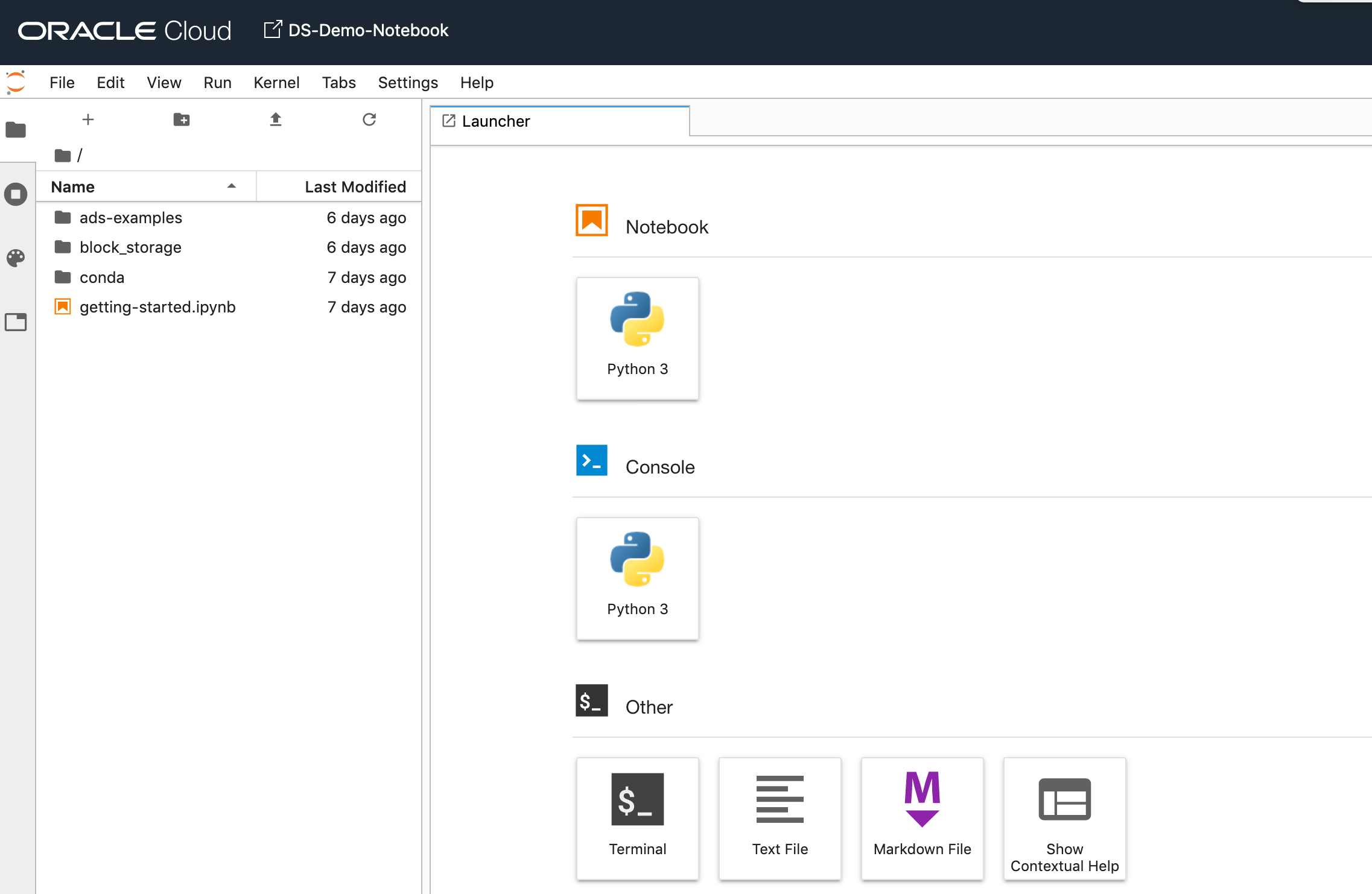
4 – Explore the Notebook Environment
The Notebook comes pre-loaded with lots of goodies.
The menu on the left-hand side provides a directory with lots of sample Notebooks, access to the block storage and a sample getting started Notebook.

When you are ready to create your own Notebook you can click on the icon for that.

Or if you already have a Notebook, created elsewhere, you can load that into your OCI Data Science environment.

The uploaded Notebook will appear in the list on the left-hand side of the screen.
Data Science (The MIT Press Essential Knowledge series) – available in English, Korean and Chinese
Back in the middle of 2018 MIT Press published my Data Science book, co-written with John Kelleher. It book was published as part of their Essentials Series.
During the few months it was available in 2018 it became a best seller on Amazon, and one of the top best selling books for MIT Press. This happened again in 2019. Yes, two years running it has been a best seller!
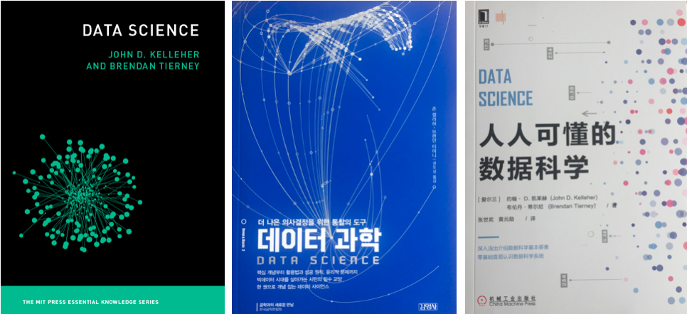
2020 kicks off with the book being translated into Korean and Chinese. Here are the covers of these translated books.


The Japanese and Turkish translations will be available in a few months!
Go get the English version of the book on Amazon in print, Kindle and Audio formats.
This book gives a concise introduction to the emerging field of data science, explaining its evolution, relation to machine learning, current uses, data infrastructure issues and ethical challenge the goal of data science is to improve decision making through the analysis of data. Today data science determines the ads we see online, the books and movies that are recommended to us online, which emails are filtered into our spam folders, even how much we pay for health insurance.
Go check it out.
Scottish Whisky Data Set – Updated
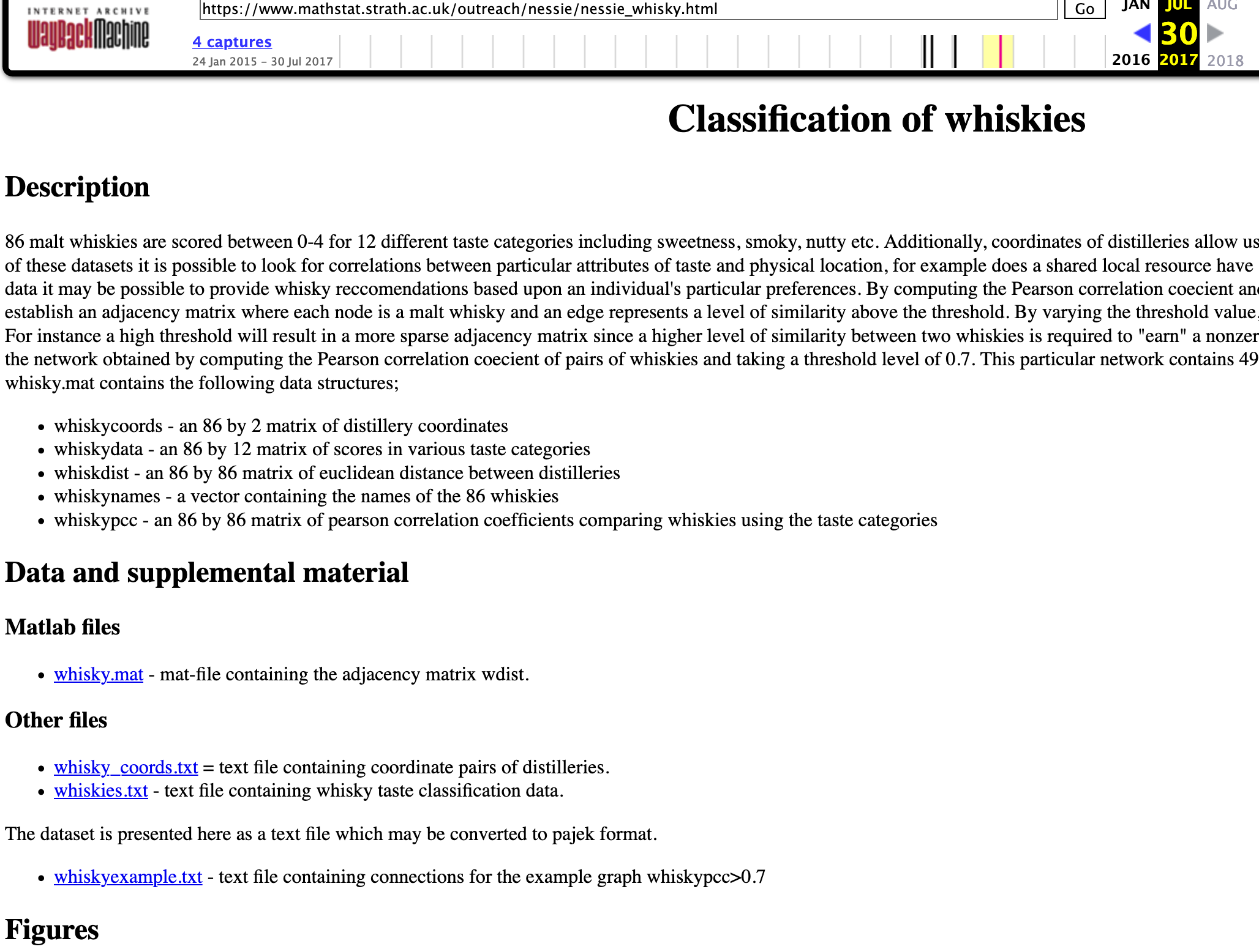
The Scottish Whiskey data set consist of tasting notes and evaluations from 86 distilleries around Scotland. This data set has been around a long time andwas a promotional site for a book, Whisky Classified: Choosing Single Malts by Flavour. Written by David Wishart of the University of Saint Andrews, the book had its most recent printing in February 2012.
I’ve been using this data set in one of my conference presentations (Planning my Summer Vacation), but to use this data set I need to add 2 new attributes/features to the data set. Each of the attributes are listed below and the last 2 are the attributes I added. These were added to include the converted LAT and LONG comparable with Google Maps and other similar mapping technology.
Attributes include:
- RowID
- Distillery
- Body
- Sweetness
- Smoky
- Medicinal
- Tobacco
- Honey
- Spicy
- Winey
- Nutty,
- Malty,
- Fruity,
- Floral,
- Postcode,
- Latitude,
- Longitude
- lat — newly added
- long — newly added
Here is the link to download and use this updated Scottish Whisky data set.
The original website is no longer available but if you have a look at the Internet Archive you will find the website.
#GE2020 Analysing Party Manifestos using Python
The general election is underway here in Ireland with polling day set for Saturday 8th February. All the politicians are out campaigning and every day the various parties are looking for publicity on whatever the popular topic is for that day. Each day is it a different topic.
Most of the political parties have not released their manifestos for the #GE2020 election (as of date of this post). I want to use some simple Python code to perform some analyse of their manifestos. As their new manifestos weren’t available (yet) I went looking for their manifestos from the previous general election. Michael Pidgeon has a website with party manifestos dating back to the early 1970s, and also has some from earlier elections. Check out his website.
I decided to look at manifestos from the 4 main political parties from the 2016 general election. Yes there are other manifestos available, and you can use the Python code, given below to analyse those, with only some minor edits required.
The end result of this simple analyse is a WordCloud showing the most commonly used words in their manifestos. This is graphical way to see what some of the main themes and emphasis are for each party, and also allows us to see some commonality between the parties.
Let’s begin with the Python code.
1 – Initial Setup
There are a number of Python Libraries available for processing PDF files. Not all of them worked on all of the Part Manifestos PDFs! It kind of depends on how these files were generated. In my case I used the pdfminer library, as it worked with all four manifestos. The common library PyPDF2 didn’t work with the Fine Gael manifesto document.
import io
import pdfminer
from pprint import pprint
from pdfminer.converter import TextConverter
from pdfminer.pdfinterp import PDFPageInterpreter
from pdfminer.pdfinterp import PDFResourceManager
from pdfminer.pdfpage import PDFPage

#directory were manifestos are located
wkDir = '.../General_Election_Ire/'

#define the names of the Manifesto PDF files & setup party flag
pdfFile = wkDir+'FGManifesto16_2.pdf'
party = 'FG'
#pdfFile = wkDir+'Fianna_Fail_GE_2016.pdf'
#party = 'FF'
#pdfFile = wkDir+'Labour_GE_2016.pdf'
#party = 'LB'
#pdfFile = wkDir+'Sinn_Fein_GE_2016.pdf'
#party = 'SF'
All of the following code will run for a given manifesto. Just comment in or out the manifesto you are interested in. The WordClouds for each are given below.
2 – Load the PDF File into Python
The following code loops through each page in the PDF file and extracts the text from that page.
I added some addition code to ignore pages containing the Irish Language. The Sinn Fein Manifesto contained a number of pages which were the Irish equivalent of the preceding pages in English. I didn’t want to have a mixture of languages in the final output.
SF_IrishPages = [14,15,16,17,18,19,20,21,22,23,24]
text = ""

pageCounter = 0
resource_manager = PDFResourceManager()
fake_file_handle = io.StringIO()
converter = TextConverter(resource_manager, fake_file_handle)
page_interpreter = PDFPageInterpreter(resource_manager, converter)

for page in PDFPage.get_pages(open(pdfFile,'rb'), caching=True, check_extractable=True):
    if (party == 'SF') and (pageCounter in SF_IrishPages):
        print(party+' - Not extracting page - Irish page', pageCounter)
    else:
        print(party+' - Extracting Page text', pageCounter)
        page_interpreter.process_page(page)

        text = fake_file_handle.getvalue()

    pageCounter += 1

print('Finished processing PDF document')
converter.close()
fake_file_handle.close()
FG - Extracting Page text 0
FG - Extracting Page text 1
FG - Extracting Page text 2
FG - Extracting Page text 3
FG - Extracting Page text 4
FG - Extracting Page text 5
...
3 – Tokenize the Words
The next step is to Tokenize the text. This breaks the text into individual words.
from nltk.tokenize import word_tokenize
from nltk.corpus import stopwords
tokens = []

tokens = word_tokenize(text)

print('Number of Pages =', pageCounter)
print('Number of Tokens =',len(tokens))
Number of Pages = 140
Number of Tokens = 66975
4 – Filter words, Remove Numbers & Punctuation
There will be a lot of things in the text that we don’t want included in the analyse. We want the text to only contain words. The following extracts the words and ignores numbers, punctuation, etc.
#converts to lower case, and removes punctuation and numbers
wordsFiltered = [tokens.lower() for tokens in tokens if tokens.isalpha()]
print(len(wordsFiltered))
print(wordsFiltered)
58198
['fine', 'gael', 'general', 'election', 'manifesto', 's', 'keep', 'the', 'recovery', 'going', 'gaelgeneral', 'election', 'manifesto', 'foreward', 'from', 'an', 'taoiseach', 'the', 'long', 'term', 'economic', 'three', 'steps', 'to', 'keep', 'the', 'recovery', 'going', 'agriculture', 'and', 'food', 'generational',
...
As you can see the number of tokens has reduced from 66,975 to 58,198.
5 – Setup Stop Words
Stop words are general words in a language that doesn’t contain any meanings and these can be removed from the data set. Python NLTK comes with a set of stop words defined for most languages.
#We initialize the stopwords variable which is a list of words like
#"The", "I", "and", etc. that don't hold much value as keywords
stop_words = stopwords.words('english')
print(stop_words)
['i', 'me', 'my', 'myself', 'we', 'our', 'ours', 'ourselves', 'you', "you're", "you've", "you'll", "you'd", 'your', 'yours', 'yourself',
....
Additional stop words can be added to this list. I added the words listed below. Some of these you might expect to be in the stop word list, others are to remove certain words that appeared in the various manifestos that don’t have a lot of meaning. I also added the name of the parties and some Irish words to the stop words list.
#some extra stop words are needed after examining the data and word cloud
#these are added
extra_stop_words = ['ireland','irish','ł','need', 'also', 'set', 'within', 'use', 'order', 'would', 'year', 'per', 'time', 'place', 'must', 'years', 'much', 'take','make','making','manifesto','ð','u','part','needs','next','keep','election', 'fine','gael', 'gaelgeneral', 'fianna', 'fáil','fail','labour', 'sinn', 'fein','féin','atá','go','le','ar','agus','na','ár','ag','haghaidh','téarnamh','bplean','page','two','number','cothromfor']
stop_words.extend(extra_stop_words)
print(stop_words)
Now remove these stop words from the list of tokens.
# remove stop words from tokenised data set
filtered_words = [word for word in wordsFiltered if word not in stop_words]
print(len(filtered_words))
print(filtered_words)
31038
['general', 'recovery', 'going', 'foreward', 'taoiseach', 'long', 'term', 'economic', 'three', 'steps', 'recovery', 'going', 'agriculture', 'food',
The number of tokens is reduced to 31,038
6 – Word Frequency Counts
Now calculate how frequently these words occur in the list of tokens.
#get the frequency of each word
from collections import Counter

# count frequencies
cnt = Counter()
for word in filtered_words:
cnt[word] += 1

print(cnt)
Counter({'new': 340, 'support': 249, 'work': 190, 'public': 186, 'government': 177, 'ensure': 177, 'plan': 176, 'continue': 168, 'local': 150,
...
7 – WordCloud
We can use the word frequency counts to add emphasis to the WordCloud. The more frequently it occurs the larger it will appear in the WordCloud.
#create a word cloud using frequencies for emphasis
from wordcloud import WordCloud
import matplotlib.pyplot as plt

wc = WordCloud(max_words=100, margin=9, background_color='white',
scale=3, relative_scaling = 0.5, width=500, height=400,
random_state=1).generate_from_frequencies(cnt)

plt.figure(figsize=(20,10))
plt.imshow(wc)
#plt.axis("off")
plt.show()

#Save the image in the img folder:
wc.to_file(wkDir+party+"_2016.png")
The last line of code saves the WordCloud image as a file in the directory where the manifestos are located.
8 – WordClouds for Each Party

Remember these WordClouds are for the manifestos from the 2016 general election.
When the parties have released their manifestos for the 2020 general election, I’ll run them through this code and produce the WordClouds for 2020. It will be interesting to see the differences between the 2016 and 2020 manifesto WordClouds.
Demographics vs Psychographics for Machine Learning
When preparing data for data science, data mining or machine learning projects you will create a data set that describes the various characteristics of the subject or case record. Each attribute will contain some descriptive information about the subject and is related to the target variable in some way.
In addition to these attributes, the data set will be enriched with various other internal/external data to complete the data set.
Some of the attributes in the data set can be grouped under the heading of Demographics. Demographic data contains attributes that explain or describe the person or event each case record is focused on. For example, if the subject of the case record is based on Customer data, this is the “Who” the demographic data (and features/attributes) will be about. Examples of demographic data include:
- Age range
- Marital status
- Number of children
- Household income
- Occupation
- Educational level
These features/attributes are typically readily available within your data sources and if they aren’t then these name be available from a purchased data set.
Additional feature engineering methods are used to generate new features/attributes that express meaning is different ways. This can be done by combining features in different ways, binning, dimensionality reduction, discretization, various data transformations, etc. The list can go on.
The aim of all of this is to enrich the data set to include more descriptive data about the subject. This enriched data set will then be used by the machine learning algorithms to find the hidden patterns in the data. The richer and descriptive the data set is the greater the likelihood of the algorithms in detecting the various relationships between the features and their values. These relationships will then be included in the created/generated model.
Another approach to consider when creating and enriching your data set is move beyond the descriptive features typically associated with Demographic data, to include Pyschographic data.
Psychographic data is a variation on demographic data where the feature are about describing the habits of the subject or customer. Demographics focus on the “who” while psycographics focus on the “why”. For example, a common problem with data sets is that they describe subjects/people who have things in common. In such scenarios we want to understand them at a deeper level. Psycographics allows us to do this. Examples of Psycographics include:
- Lifestyle activities
- Evening activities
- Purchasing interests – quality over economy, how environmentally concerned are you
- How happy are you with work, family, etc
- Social activities and changes in these
- What attitudes you have for certain topic areas
- What are your principles and beliefs
The above gives a far deeper insight into the subject/person and helps to differentiate each subject/person from each other, when there is a high similarity between all subjects in the data set. For example, demographic information might tell you something about a person’s age, but psychographic information will tell you that the person is just starting a family and is in the market for baby products.
I’ll close with this. Consider the various types of data gathering that companies like Google, Facebook, etc perform. They gather lots of different types of data about individuals. This allows them to build up a complete and extensive profile of all activities for individuals. They can use this to deliver more accurate marketing and advertising. For example, Google gathers data about what places to visit throughout a data, they gather all your search results, and lots of other activities. They can do a lot with this data. but now they own Fitbit. Think about what they can do with that data and particularly when combined with all the other data they have about you. What if they had access to your medical records too! Go Google this ! You will find articles about them now having access to your health records. Again combine all of the data from these different data sources. How valuable is that data?
Managing imbalanced Data Sets with SMOTE in Python
When working with data sets for machine learning, lots of these data sets and examples we see have approximately the same number of case records for each of the possible predicted values. In this kind of scenario we are trying to perform some kind of classification, where the machine learning model looks to build a model based on the input data set against a target variable. It is this target variable that contains the value to be predicted. In most cases this target variable (or feature) will contain binary values or equivalent in categorical form such as Yes and No, or A and B, etc or may contain a small number of other possible values (e.g. A, B, C, D).
For the classification algorithm to perform optimally and be able to predict the possible value for a new case record, it will need to see enough case records for each of the possible values. What this means, it would be good to have approximately the same number of records for each value (there are many ways to overcome this and these are outside the score of this post). But most data sets, and those that you will encounter in real life work scenarios, are never balanced, as in having a 50-50 split. What we typically encounter might be a 90-10, 98-2, etc type of split. These data sets are said to be imbalanced.

The image above gives examples of two approaches for creating a balanced data set. The first is under-sampling. This involves reducing the class that contains the majority of the case records and reducing it to match the number of case records in the minor class. The problems with this include, the resulting data set is too small to be meaningful, the case records removed could contain important records and scenarios that the model will need to know about.
The second example is creating a balanced data set by increasing the number of records in the minority class. There are a few approaches to creating this. The first approach is to create duplicate records, from the minor class, until such time as the number of case records are approximately the same for each class. This is the simplest approach. The second approach is to create synthetic records that are statistically equivalent of the original data set. A commonly technique used for this is called SMOTE, Synthetic Minority Oversampling Technique. SMOTE uses a nearest neighbors algorithm to generate new and synthetic data we can use for training our model. But one of the issues with SMOTE is that it will not create sample records outside the bounds of the original data set. As you can image this would be very difficult to do.
The following examples will illustrate how to perform Under-Sampling and Over-Sampling (duplication and using SMOTE) in Python using functions from Pandas, Imbalanced-Learn and Sci-Kit Learn libraries.
NOTE: The Imbalanced-Learn library (e.g. SMOTE)requires the data to be in numeric format, as it statistical calculations are performed on these. The python function get_dummies was used as a quick and simple to generate the numeric values. Although this is perhaps not the best method to use in a real project. With the other sampling functions can process data sets with a sting and numeric.
Data Set: Is the Portuaguese Banking data set and is available on the UCI Data Set Repository, and many other sites. Here are some basics with that data set.
import warnings

import pandas as pd
import numpy as np
import matplotlib.pyplot as plt
get_ipython().magic('matplotlib inline')

bank_file = ".../bank-additional-full.csv"

# import dataset
df = pd.read_csv(bank_file, sep=';',)

# get basic details of df (num records, num features)
df.shape
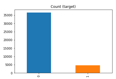
df['y'].value_counts() # dataset is imbalanced with majority of class label as "no".
no     36548
yes     4640
Name: y, dtype: int64
#print bar chart
df.y.value_counts().plot(kind='bar', title='Count (target)');
Example 1a – Down/Under sampling the majority class y=1 (using random sampling)
count_class_0, count_class_1 = df.y.value_counts()

# Divide by class
df_class_0 = df[df['y'] == 0] #majority class
df_class_1 = df[df['y'] == 1] #minority class

# Sample Majority class (y=0, to have same number of records as minority calls (y=1)
df_class_0_under = df_class_0.sample(count_class_1)
# join the dataframes containing y=1 and y=0
df_test_under = pd.concat([df_class_0_under, df_class_1])

print('Random under-sampling:')
print(df_test_under.y.value_counts())
print("Num records = ", df_test_under.shape[0])

df_test_under.y.value_counts().plot(kind='bar', title='Count (target)');

Example 1b – Down/Under sampling the majority class y=1 using imblearn
from imblearn.under_sampling import RandomUnderSampler

X = df_new.drop('y', axis=1)
Y = df_new['y']

rus = RandomUnderSampler(random_state=42, replacement=True)
X_rus, Y_rus = rus.fit_resample(X, Y)

df_rus = pd.concat([pd.DataFrame(X_rus), pd.DataFrame(Y_rus, columns=['y'])], axis=1)

print('imblearn over-sampling:')
print(df_rus.y.value_counts())
print("Num records = ", df_rus.shape[0])

df_rus.y.value_counts().plot(kind='bar', title='Count (target)');
[same results as Example 1a]
Example 1c – Down/Under sampling the majority class y=1 using Sci-Kit Learn
from sklearn.utils import resample

print("Original Data distribution")
print(df['y'].value_counts())

# Down Sample Majority class
down_sample = resample(df[df['y']==0],
replace = True, # sample with replacement
n_samples = df[df['y']==1].shape[0], # to match minority class
random_state=42) # reproducible results

# Combine majority class with upsampled minority class
train_downsample = pd.concat([df[df['y']==1], down_sample])

# Display new class counts
print('Sci-Kit Learn : resample : Down Sampled data set')
print(train_downsample['y'].value_counts())
print("Num records = ", train_downsample.shape[0])
train_downsample.y.value_counts().plot(kind='bar', title='Count (target)');
[same results as Example 1a]
Example 2 a – Over sampling the minority call y=0 (using random sampling)
df_class_1_over = df_class_1.sample(count_class_0, replace=True)
df_test_over = pd.concat([df_class_0, df_class_1_over], axis=0)

print('Random over-sampling:')
print(df_test_over.y.value_counts())

df_test_over.y.value_counts().plot(kind='bar', title='Count (target)');
Random over-sampling:
1    36548
0    36548
Name: y, dtype: int64

Example 2b – Over sampling the minority call y=0 using SMOTE
from imblearn.over_sampling import SMOTE

print(df_new.y.value_counts())
X = df_new.drop('y', axis=1)
Y = df_new['y']

sm = SMOTE(random_state=42)
X_res, Y_res = sm.fit_resample(X, Y)

df_smote_over = pd.concat([pd.DataFrame(X_res), pd.DataFrame(Y_res, columns=['y'])], axis=1)

print('SMOTE over-sampling:')
print(df_smote_over.y.value_counts())

df_smote_over.y.value_counts().plot(kind='bar', title='Count (target)');
[same results as Example 2a]
Example 2c – Over sampling the minority call y=0 using Sci-Kit Learn
from sklearn.utils import resample

print("Original Data distribution")
print(df['y'].value_counts())

# Upsample minority class
train_positive_upsample = resample(df[df['y']==1],
replace = True, # sample with replacement
n_samples = train_zero.shape[0], # to match majority class
random_state=42) # reproducible results

# Combine majority class with upsampled minority class
train_upsample = pd.concat([train_negative, train_positive_upsample])

# Display new class counts
print('Sci-Kit Learn : resample : Up Sampled data set')
print(train_upsample['y'].value_counts())
train_upsample.y.value_counts().plot(kind='bar', title='Count (target)');
[same results as Example 2a]
Why Data Science projects fail
Over the past few weeks or months (maybe even years) I’ve had several conversations with various people about why Data Science (or whatever you want to call it) projects fail or never really get started.
Before we go any further perhaps we need to define what ‘fail’ means in these conversations. Typically fail means that the project doesn’t deliver what was hoped for, it got bogged down is some technical or political issues, it did not deliver useful results, and more typically it is run once (or a couple of times) and never run again. You get the idea.
The following points outline some of the most typical reasons why Data Science projects fail, but this is not an exhaustive list. This list is just some of the most typical reason.
- We need Big Data: It seems like everything that you read says you need Big Data for your data science project. Firstly what big data means to one person or company can be very different to what it means for another person/company. One possible definition is that it might include all the various social media and log type of data. If you don’t have all of this data then no big deal. You can still do data science projects. You have lots and lots of other data. The data that you generate every day for the general running of your business. You can use that. If you have some history of this data going back over a few months or a couple of years then even better (and most of you will say Yes I have that data). Work with the data that you already have, that you already understand, that you are already using, etc and use that data to see if you can gain extra insights that will have some value to your business (it needs to have value otherwise whats the point). Some people call this everyday type of data you have, ‘Small Data’. Big Data or Small Data are really bad terms. It is just Data. Let us work with data we already have and incrementally add in newer data (from your typical ‘Big Data’ sources) with each iteration of the data science project.
- We need Big Technology: This kind of follows on from the mistake of believing we need Big Data to do our data science projects. As most companies will be working with the data that they already have, and you will have various technology solutions in place to manage this data. Then do we really need Big Data Technology solutions for our Data Science projects? Technologies like Hadoop and everything that goes along with it. The simple answer is ‘No You Don’t’. Now don’t get me wrong. These technologies are important with it comes to managing Big Data, but you don’t needs these to perform your data science projects. Many, many companies both large and small are performing data science projects using their existing technology solutions and have perhaps just added some analytics tools to support their project using the data that they are already managing. Most companies have databases to store and manage their data. You can use your analytics software to work with the data in these database to analyse, model and predict. Any results that are produced can be easily integrated back into these databases and the results can then be used by various groups within your organisation. Use the technologies you have, that you understand, that you can use to the max, supplemented with some newer analytics software that works with all of these for your data science projects. (An example: one project I’ve worked on included a retail organisation for one of the largest countries in the work. I was working with 3 years of sales data. Is this big data? I was able to use my laptop to perform advanced analytics on all their data)
- Old School Data Science: Give me all your data, I’ll analyse it and tell you what is happening. Unfortunately this kind of phrases are still very common. They are common and considered out of date 20 years ago when I worked on my first data science project (it wasn’t called data science back then). If you do come across someone saying this to you, I would question their ability to deliver anything. If it was me, I would just say ‘No thank you’, and move onto someone else. You as a company will already know a lot of what is happening in your business, what data is currently being used for and any potential areas where you know advanced analytics and data science can help. You will know that the focus areas should be and how good or not your data is. You need someone who can help you to identify the key areas and what data science techniques can be used to help you to gain (a possible) greater insight into what is happening.
- No clear objective or business question/problem and no measurable outcomes: In a way this is very similar to the previous point. You don’t get into your car each morning and start driving, with the eventual hope that you arrive at work on time. No, you plan what you want to do (get to work), how you are going to get then (using your car) and when you want to get there by (your work start time). Using these you then plan out what is the best route you need to take to get to work, in the most efficient way you can, using your knowledge and experience of the road network, supplemented by traffic reports and making adjustments as necessary, to ensure that you get to work on time. This is exactly the same for data science projects. You need a good clear objective, that can be broken down into distinct problems, that will each require a specific set of advanced analytics to generate a measurable outcome. The measurable outcomes should allow you to measure if the advanced analytics actually gives you a valuable return. For example if you predict that you can increase sales by 3%, this sound good. But if the cost of implementing the solution is treating any the profit generated then you might decide that this solution is not worth continuing with.
- Not productionalising the outcomes: This point follows on from the previous two points. A lot of what you read and a lot of what I’ve seen is that Data Science looks are discovering some new (and actionable) insights. But that is where the discussion ends. As if a report is produced that makes a recommendation or a list of customers to target, and that is it. What happens to your data science project then. It really gets canned or you might be told that we will come back to it in a few months (and possibly a year) from now. This is not what you really want. Why? because when you finally remember to come back to review the project and to do another run, the people who where involved in the original project have moved on or are not available. It then become too difficult to start over again and that is when the data science project fails. I’ve used the word ‘productionalising’ (is that a real word?) What I mean by that is that we need to take our data science project and build it into our every day applications and processes. For example if we build a customer risk model for loans in a bank. This should be built into the application that captures the loan application by the customer. That way when the bank employee is entering the loan application they can be given live feedback. They can then use this live feedback to address any issues with the customer. What can be typical is that this is discovered some weeks later when the loan has already been approved. We need to automate the use of our data science work. Another example is fraud detection. I know of several companies who have fraud detection measures in place. It can take them 4-6 weeks to identify a potential fraud case that needs investigation. Using data science and building this into their transaction monitoring systems they can now detect potential fraud cases in near real time )no big data architectures being used). By automating it we get quicker response and take actions at the right time. The quicker we can react the more money we can make or save. This is an area that a lot of companies are now focusing on when they are looking at data science project as this is they way that they can get a quicker return on their investment in their data science projects.
- Very little senior management support: I think most of the data science projects are supported by senior management to some extent. The more successful the data science project the more involved the senior managers are and the more they understand of what these projects can potentially deliver. But with the ever changing and evolving world of IT most of the senior managers are very focused on the here and now, keeping the lights on, making sure their day-to-day applications are up and running, the backups and recovery processes are in place (and tested), and future proofing their application. It is well known that very little time and resources (human and money) are available for adding new functionality. Most of what I’ve mentioned is very IT related and perhaps the IT managers are not the most suitable people to sponsor data science projects. I’ve already some of the reasons but sometimes IT can get a bit caught up with the technology and trying to use the newest thing. Some of the most successful projects I’ve worked on have had senior managers from a business function. They will not be focused on the technology but on the processes around the data science project and how the outputs of the data science project can be used. The more focused they are on this the more successful the project will be. They will then act as the key to informing (and selling) the rest of the business on the success of the project. This in turn create more and more data scicene projects and will keep you busy for a long time to come
- Ticking the box: Unfortunately I’ve seen this in way too many companies. Board level or the senior management team have hear about data science and all the magic that is can produce. The message is then passed down through the organisation that we need to be doing more and more of this. A business unit is chosen as for the pilot project. The pilot is completed, successfully, and the good news message is fed back up the ladder. But that is when enthusiasm ends. We have done a data science project, it was successful and now lets move on to the next thing. I’ve seen pilot or POC project that have proven to potentially save $10+M a year with a cost of $100K per year, being canned. Yes I’ve been told this is fantastic, this is beyond our wildest dreams. Only for nothing else to happen.
- The data is no good: You need data, you need historical data. The more you have more more useful it will be for the data science project. But what if the data is of poor quality? How can this happen? Well it can happen very frequently. You may have applications that are poorly designed, that have a very poor data model, the staff are not trained correctly to ensure that good data gets entered, etc. etc. The list could go on and on. It is one thing for an application to capture data but if that data cannot be used for any meaningful purposes then it has very little value. Some companies have people hired that constantly inspect the data, assess the quality of the data and are then feeding back ideas on how to improve the quality of the data captured by the applications and also by the people inputting the data. Without good quality data then there is very little a data science project can do to magically convert it into good quality data. I’ve been in the situation where >90% of the data was unusable. We give them a list what improvements they needed to make and only come back to use then they have completed these and have at least 6 months of good quality data. We might be able to do something then. We never heard from them again. Also I get to talk to a lot of start ups who want to have data science build in from day one. These have very little ‘real’ data. Again I get to tell them come back to me when you have 6 months of data.
- Too much focus on descriptive analytics: Although descriptive analytics is an important step in the early stages of all data science projects, they is still a huge number of consulting and product companies who are promoting this as a data science project. Like I said descriptive analytics is an important step, but it doesn’t end there. It is just the beginning. When selecting a consulting or product company to partner with on your data science projects you need to ensure that they are offering more than just descriptive analytics. In a similar way to what I’ve mentioned in the points above, you need to look at how you can make use of these descriptive analytics and share them with the wider community in your company. But you also need to have some control over the proliferation of various visualisation tools. Descriptive analytics and visualisations is not data science or a major output of data science. It is only one part of a data science project and far more value outputs from a data science project can be achieved by using one or more of the advanced analytics methods that are available to you.
- Ignoring your BI/DW: Unfortunately when it comes to a lot of data science projects your have two very different approaches to working with the data. One approach seems to be that we will look at your data that is available in the transactional databases (and other data sources), we will then look at how to integrate and clean this data before getting onto the fund stuff of exploring and then performing the advanced analytics. This approach completely ignores the BI team and any data warehouse that might exist. If a data warehouse already exists then it probably contains all or most of the data you are going to use. Therefore you can avoid all that them spent integrating and cleaning the data. The data warehouse will have this done for you. Plus the data warehouse will have a lot more data than what the current transactional databases will contain. Please, Please, Please use the data in the data warehouse and you will find that you will save a lot of time on your data science project. In addition to the time saved you will have a lot more (possibly years of) data to work with. I always try to work with data warehouse data. When I do I can go back 5 years and build predictive models from back then. I can then roll these through various time periods and can easily measure how good the level of predictive I’m getting. I also get to see if there are any changes in the data and how they affect the models. Plus I also get to see how the various algorithms and their associated models change and evolve over time. This allows me to demonstrate to the customer how the use of data science and predictive models works with their data over the past 5 years. This build up confidence with the customer on what is being done and what can be achieved. In one case I was able to demonstrate that if they implemented my solution 5 years ago, they would have save $40+M in that time period. If I didn’t use the data warehouse I wouldn’t have been able to prove this. Needless to say the customer was very happy.
- Make up of team is wrong: You don’t need a team of PhDs: There has been lots written about what the make up of skills what your data science team should be. Back a few years ago all the talk was that you need to have people with PhDs maths, stats or related states. Plus all you needed to do was to hire one of these. We all know that this is not true but was part of the rubbish that people were talking about. We all know that you really need a team of people and perhaps you already have some of these people already employed in your company already. You have database people, you have ETL people, you have data integration people, you have data analysts, you have project managers, you have business analysts, you have domain experts, etc. How many of those people have PhDs or require a PhD to do their job. But perhaps you don’t have people with the skills of applying advanced analytic techniques to your data and business problems. Perhaps it is these people who you really need the most. Do these people really need to have a PhD? No they don’t. You need someone who knows and understands the various techniques and most importantly how to use these to solve business problems. All too often people try to show off about using a particular technique or parameter setting, or a particular formula, or graphic technique, or using a certain language over another, or what library or package is the best. Don’t engage in this. Look for people that can apply the correct technique or combination of techniques to your business problems. But despite what I said in the first two point, as your data management requirements grow you are going to need some addition people with some big data technologies.
- Communication: being able to explain what data science can do, what it is producing and relating that back to the business. Being able to work with the management team, end users and all involved to show and explain what and how the data science project can do to support their work. Most technical people are not good at this. Bus some people are and these are a very valuable resource as part of your data science team or are keen supporter of what data science can do and how it can be used to help the business developed new and interesting actionable insights.
- The output is not a report => You need to operationise/productionalise the data science project: See the point above on productionalising your data science work. The outputs should not be a report or a list of some form. With proper planning data science can become a central to all the operational systems in your company. They can help you make better and quicker decisions on how you interact with your customers, improve the efficiencies of your processes, etc. The list goes on and on. All data science projects are cyclical in nature. For example you developer a churn prediction system. You use this to interact with your customers. You are trying to change or alter their behaviour and this in turn changes them as a customer. This in turn affect the churn prediction system. It will no longer be as effective. So you will need to update it on a semi-regular basis. This could be every 3, 4, 6, or 12 months. It all depends. You can build in checks into your productionalised data science projects to detect when the predictive models need updating. This in turn helps your data science team to be more productive, with quicker turn around times of each iteration. Also with each iteration you can look to see if new data is available for you to include and use. Maybe at this point some of your big data sources are coming online with some useful data.
So when looking to start a Data Science project it is important to know a few things before you start. The following attempts to use the 5 W’s to try explains these.
- what you are doing
- why you are doing it
- who it is for and what they will gain from it
- where will it be used within your applications/processes
- when you are going to commence the project and how it will fit into strategic goals of your organisation
There has been plenty written about what magic Data Science projects will produce and bring to your organisation. You need to be careful of people who only talk about the magic. You also need to understand that it may not work or deliver what you are lead to believe. In all the projects I’ve worked on we have had some amazing results. But in one or two projects we have had results that where only a percentage or two better than what they are already doing.
Perhaps I need to write another blog post on ‘Why Data Science projects succeed’, and this will only be based on what I’ve experienced (in the real-world).
Like I said at the beginning, this is not an exhaustive list. There are many more and I’m sure you will have a few of your own. These are the typical reasons that I’ve come across in my 20 years of doing these kind of projects and long before the term data science existed.
- ← Previous
- 1
- 2

You must be logged in to post a comment.