
Oracle
Running Oracle Database on Docker on Apple M1 Chip
Click on this link to see the latest way to run Oracle 23ai Database on Docker. The instructions below are a bit obsolete, although they work for M1. To run Oracle 23ai Database on Docker on Apple Scilcon check out the instructions on this link.
This post is for you if you have an Apple M1 laptop and cannot get Oracle Database to run on Docker.
The reason Oracle Database, and lots of other software, doesn’t run on the new Apple Silicon is their new chip uses a different instruction set to what is used by Intel chips. Most of the Database vendors have come out to say they will not be porting their Databases to the M1 chip, as most/all servers out there run on x86 chips, and the cost of porting is just not worth it, as there is zero customers.
Are you using an x86 Chip computer (Windows or Macs with intel chips)? If so, follow these instructions (and ignore this post)
If you have been using Apple for your laptop for some time and have recently upgraded, you are now using the M1 chip, and you have probably found some of your software doesn’t run. In my scenario (and with many other people) you can no longer run an Oracle Database 😦
But there does seem to be a possible solution and this has been highlighted by Tom de Vroomen on his blog. A workaround is to spin up an x86 container using Colima. Tom has given some instructions on his blog, and what I list below is an extended set of instructions to get fully set up and running with Oracle on Docker on M1 chip.
1-Install Homebrew
You might have Homebrew installed, but if not run the following to install.
/bin/bash -c "$(curl -fsSL https://raw.githubusercontent.com/Homebrew/install/HEAD/install.sh)"2-Install colima
You can now install Colima using Homebrew. This might take a minute or two to run.
brew install colima3-Start colima x86 container
With Colima installed, we can now start an x86 container.
colima start --arch x86_64 --memory 4
The container will be based on x86, which is an important part of what we need. The memory is 4GB, but you can probably drop that a little.
The above command should start within a second or two.
4-Install Oracle Database for Docker
The following command will create an Oracle Database docker image using the image created by Gerald Venzi.
docker run -d -p 1521:1521 -e ORACLE_PASSWORD=<your password> -v oracle-volume:/opt/oracle/oradata gvenzl/oracle-xe
23c Database – If you want to use the 23c Database, Check out this post for the command to install
I changed <your password> to SysPassword1.
This will create the docker image and will allow for any changes to the database to be persisted after you shutdown docker. This is what you want to happen.
5-Log-in to Oracle as System
Open the docker client to see if the Oracle Database image is running. If not click on the run button.

When it finishes starting up, open the command line (see icon to the left of the run button), and log in as the SYSTEM user.
sqlplus system/SysPassword1@//localhost/XEPDB1
You are now running Oracle Database on Docker on an M1 chip laptop 🙂
6-Create new user
You shouldn’t use the System user, as that is like using root for everything. You’ll need to create a new user/schema in the database for you to use for your work. Run the following.
create user brendan identified by BTPassword1 default tablespace usersgrant connect, resource to brendan;If these run without any errors you now have your own schema in the Oracle Database on Docker (on M1 chip)
7-Connect using SQL*Plus & SQL Developer
Now let’s connect to the schema using sqlplus.
sqlplus brendan/BTPassword1@//localhost/XEPDB1That should work for you and you can now proceed using the command line tool.
If you refer to use a GUI tool then go install SQL Developer. Jeff Smith has a blog post about installing SQL Developer on M1 chip. Here is the connection screen with all the connection details entered (using the username and password given/used above)

You can now use the command line as well as SQL Developer to connect to your Oracle Database (on docker on M1).
8-Stop Docker and Colima
After you have finished using the Oracle Database on Docker you will want to shut it down until the next time you want to use it. There are two steps to follow. The first is to stop the Docker image. Just go to the Docker Desktop and click on the Stop button. It might take a few seconds for it to shutdown.
The second thing you need to do is to stop Colima.
colima stopThat’s it all done.
9-What you need to run the next time (and every time after that)
For the second and subsequent time you want to use the Oracle Docker image all you need to do is the following
(a) Start Colima
colima start --arch x86_64 --memory 4
(b) Start Oracle on Docker
Open Docker Desktop and click on the Run button [see Docker Desktop image above]
And to stop everything
(a) Stop the Oracle Database on Docker Desktop
(b) Stop Colima by running ‘colima stop’ in a terminal
Changing In-Memory size in Oracle Database
The pre-built virtual machine provided by Oracle for trying out and playing with Oracle Database comes configured to use the In-Memory option. But memory size is a little limited if you are trying to load anything slightly bigger than a tiny table into memory, for example if the table has more than a few hundred rows.
The amount of memory allocated to In-Memory can be increased to allow for more data to be loaded. There is a requirement that the VM and Database has enough memory allocated to allow this. If you don’t and increase the In-Memory size too large, you will have some problems restarting the database and VM. So proceed carefully.
For the pre-built VM, I typically allocate 4G or 8G of RAM to the VM. This in turn will give more memory to the database when it starts.
To setup In-Memory on the VM run the following:
– Open a terminal window and run this command:
sqlplus sys/oracle as sysdbaThen run these two commands
alter session set container = cdb$root;
alter system set inmemory_size = 200M scope=spfile;
Now, bounce the VM, i.e. restart the VM
In-memory will now be enabled on your Database, and you can now create/move tables in and out of in-memory.
How many Data Center Regions by Vendor?
There has been some discussions over the past weeks, months, years on which Cloud provider is the best, or the biggest, or provides the most services, or [insert some other topic]? The old answer to everything related to IT is ‘It Depends’. A recent article by CloudWars (and updated numbers by them) and some of the comments to it, and elsewhere prompted me to have a look at ‘How Many Data Center Regions do each Cloud Vendor have?’ I didn’t go looking at all possible cloud vendors, but instead kept to the main vendors consisting of Microsoft Azure, Google Cloud Platform (GCP), Oracle Cloud and Amazon Web Services (AWS). We know AWS has been around for a long long time, and seems to gather most of the attention and focus within the developer community, etc, you’d expect them to be the biggest. Well, the results from my investigation does not support this.
Now, it is important to remember when reading the results presented below that these are from a particular point in time, and that is the date of this blog post. If you are reading this some time later, the actual number of data centers will be different and will be larger.
When looking at the data, as presented on each vendors website (see link to each vendor below), most list some locations coming in the future. It’s really impressive to see the number of “coming soon” locations. These “coming soon” locations are not included below (as of blog post date).
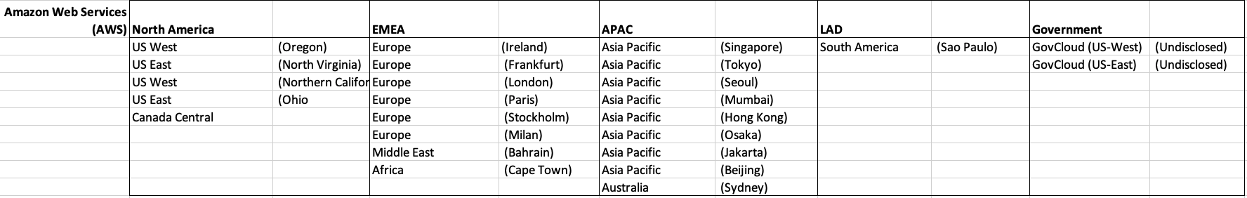
Before showing a breakdown for each vendor the following table gives the total number of data center regions for each vendor.
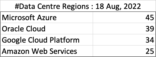
The numbers presented in the above table are different to does presented in the original CloudWars article or their updated numbers. If you look at the comments on that article and the comments on LinkedIn, you will see there was some disagreement of on their numbers. The problem is a data quality one, and vendors presenting their list of data centers in different parts of their website and documentation. Data quality and consistency is always a challenge, and particularly so when publishing data on vendor blogs, documentation and various websites. Indeed, the data I present in this post will be out of date within a few days/weeks. I’ve also excluded locations marked as ‘coming soon’ (see Azure listing).
Looking at the numbers in the above table can be a little surprising, particularly if you look at AWS, and then look at the difference in numbers between AWS and Azure and even Oracle. Very soon Azure will have double the number of data center regions when compared to AWS.
What do these numbers tell you? Based on just these numbers it would appear that Azure and Oracle Cloud are BIG cloud providers, and are much bigger than AWS. But maybe AWS has data centers that are way way bigger than those two vendors. It can be a little challenging to know the size and scale of each data center. Maybe they are going after different types of customers? With the roll out of Cloud over the past few years, there has been numerous challenges from legal and sovereign related issues requiring data to be geographically located within a country or geographic region. Most of these restrictions apply to larger organizations in the financial, insurance, and government related, etc. Given the historical customer base of Microsoft and Oracle, maybe this is driving their number of data center regions.
In more recent times there has been a growing interest, and in some sectors a growing need for organizations to be multi-cloud. Given the number of data center regions, for Azure and Oracle, and commonality in their geographic locations, it isn’t surprising to see the recent announcement from Azure and Oracle of their interconnect agreement and making the Oracle Database Service available (via interconnect) from Azure. I’m sure we will see more services being shared between these two vendors, and other might join in doing something similar.
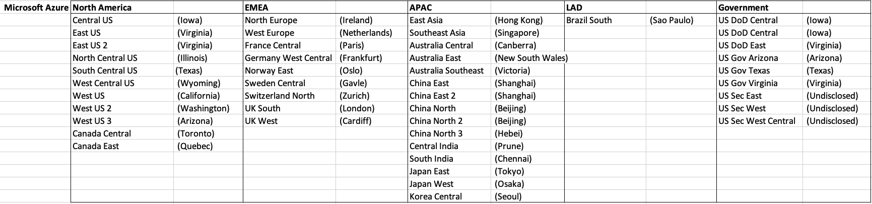
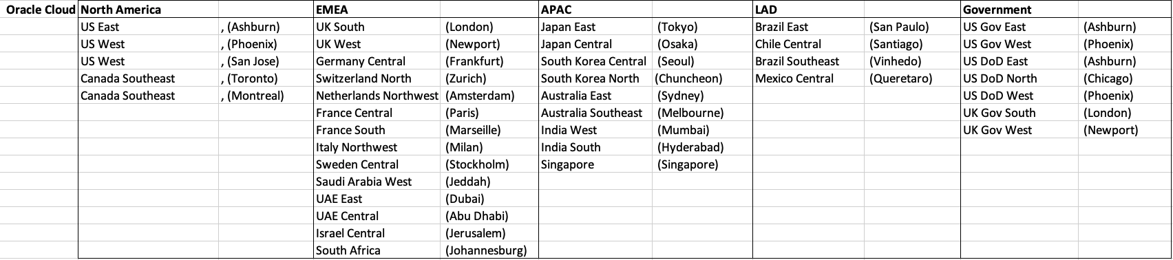
Let’s get back to the numbers and data for each Vendor. I’ve also included a link to the Vendor website where these data was obtained. (just remember these are based on date of blog post)
When you look at the Azure website listing the location, at first look it might appear they have many more locations. When you look closer at these, some/many of them are listed as ‘coming soon’. These ‘coming soon’ locations are not included in the above and below tables.
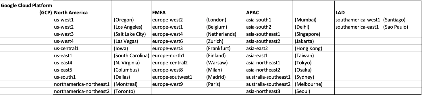
GCP doesn’t list and Government data center regions.
Oracle on AWS costs
In a previous post I walked through the steps of setting up an Oracle Database on AWS RDS. It was a very simple and straight forward process. The only thing to watch out for was to open the network to allow traffic in and out. I also showed how to connect SQL Developer to that database.
I’ve been using it for a few days and needed to move onto other things for a few days. I could leave the Database up and running during this period or I could shut down the Database to save a few dollars/euro. It also gave me a chance to see how much this database cloud instance is costing me. In my previous post, it was estimated to cost about 0.89c per day.
Before we look at the Actual/Real costs, let’s walk through the steps of shutting down the database.
To stop the database, click on the Actions button on the top right hand side of the screen, just above the database summary details. You will get a confirmation window/box appearing, see image below, asking you to confirm by clicking ‘Yes, Stop Now’.
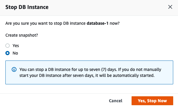
It will take a few minutes for this shutdown to complete and in my case it took approx. 8 minutes, which was a little surprising as no one was using it at the time. You might need to refresh the webpage to see this change.

That’s all very simple, but it does give you a warning about the stopped database instance. It will be restarted in 7 days time! So if this is a database you will occasionally use, then you will need to carefully manage this particular feature, otherwise you will end up with the database automatically starting and you will be paying for this.
What about the Costs?
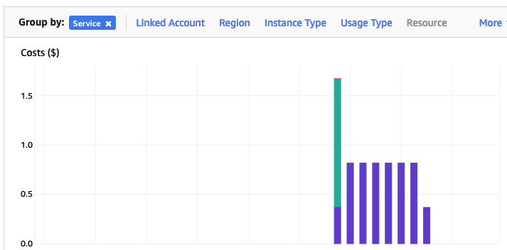
The costs for running this service can be found in the AWS Cost Management page. Here we can see the database was running for 7 and a bit days before I shut it down, and we can see the daily cost was 0.82c. Two things note about these costs. There was larger cost for the first day. Most of this cost was associated with the setup and configuration of the database service. The second thing to note is the costs listed in this console do not include taxes.
A got the bill for this usage, and it came to $6.94, consisting of $5.64 for usage (approx. 75c per day) and $1.30 in taxes/vat. Not a lot considering some cloud services, but comes out at approx 92.5c per day, which is a little more than the estimated cost when the service was being created. A small example of what can happen between the “in theory” cost of cloud versus the actual costs.
Database Vendors on Twitter, Slack, downloads, etc.
Each year we see some changes in the positioning of the most popular databases on the market. “The most popular” part of that sentence can be the most difficult to judge. There are lots and lots of different opinions on this and ways of judging them. There are various sites giving league tables, and even with those some people don’t agree with how they perform their rankings.
The following table contains links for some of the main Database engines including download pages, social media links, community support sites and to the documentation.
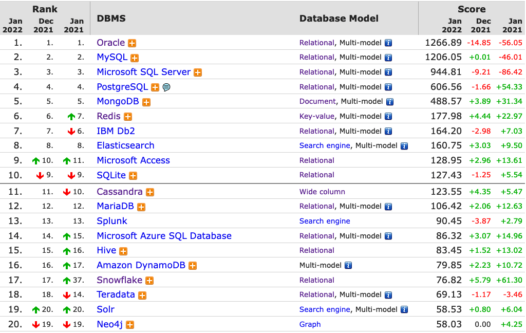
One of the most common sites is DB-Engines, and another is TOPDB Top Database index. The images below show the current rankings/positions of the database vendors (in January 2022).
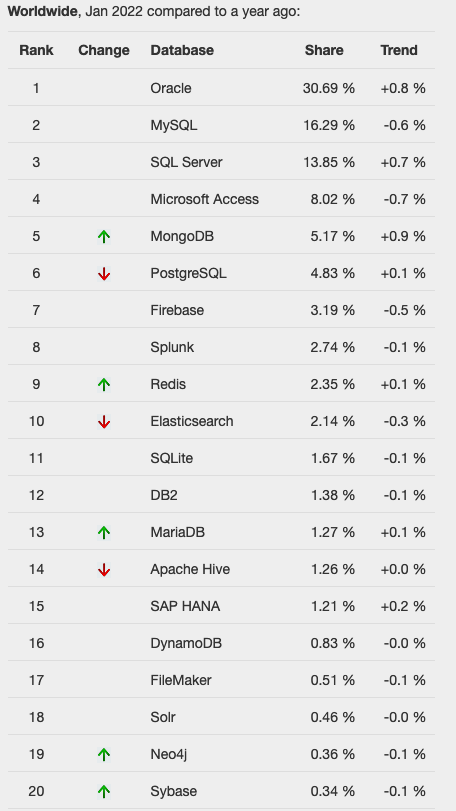
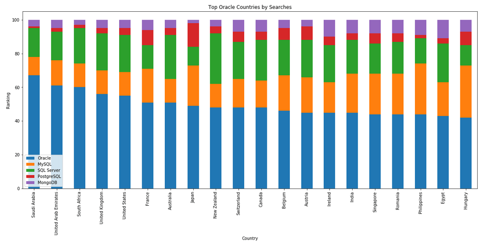
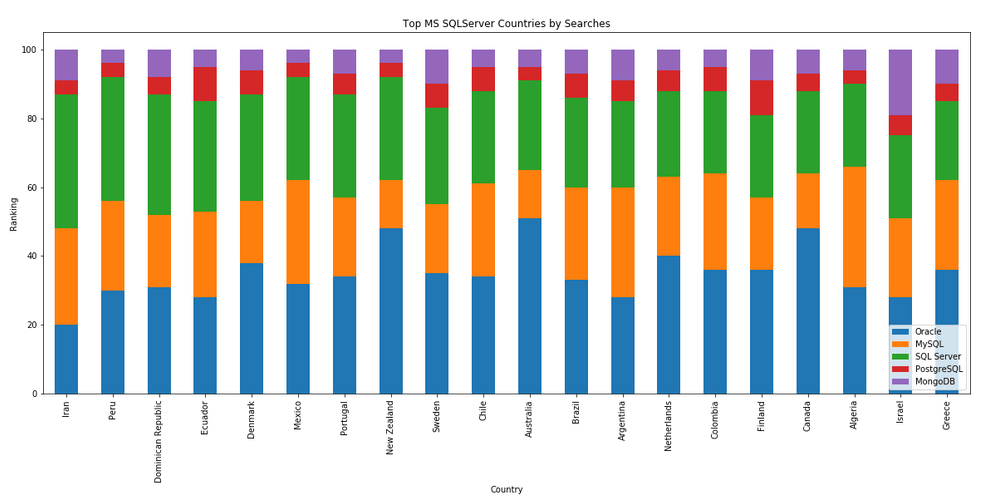
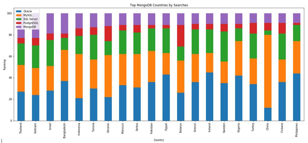
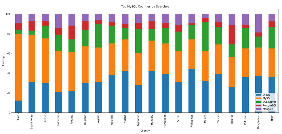
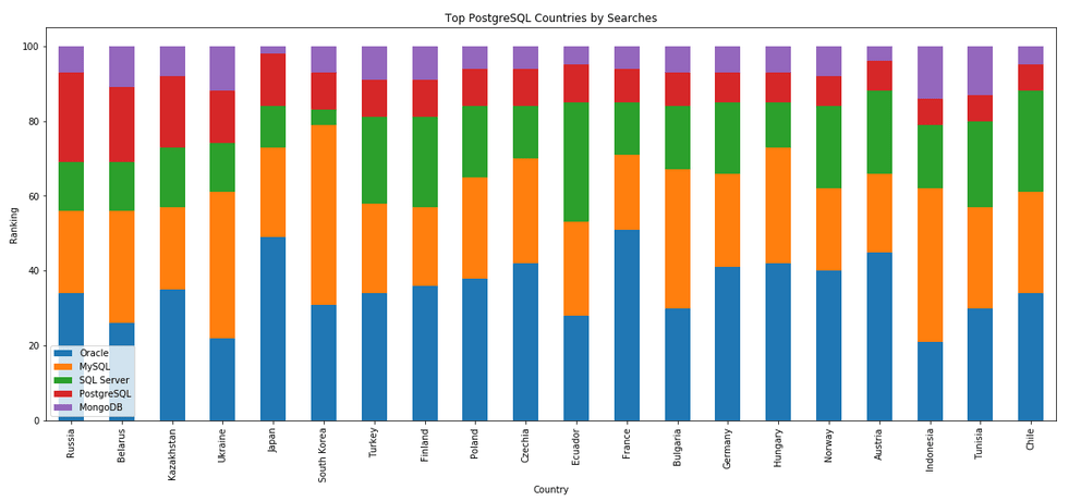
I’ve previously written about using the Python pytrends package to explore the relative importance of the different Database engines. The results from pytrends gives results based on number of searches etc in Google. Check out that Blog Post. I’ve rerun the same code for 2021, and the following gallery displays charts for each Database based on their popularity. This will allow you to see what countries are most popular for each Database and how that relates to the other databases. For these charts I’ve included Oracle, MySQL, SQL Server, PostgreSQL and MongoDB, as these are the top 5 Databases from DB-Engines.
Using SQL to create some festive Christmas Trees
Here are a few examples I found on the “great internet” of how SQL can be used to create some festive Christmas cheer and fun. See links to the original posts. Most of the examples shown below have been run on Oracle 21c Docker image, or on SQL Server or MySQL.
Our first example comes from Gerald Venzi who posted this on twitter. See later in the post for Christmas trees created using similar SQL queries.
WITH tree(lev, xmas) AS (
   SELECT 1 lev, RPAD(' ', 10, ' ') || '*' xmas
   FROM dual
   UNION ALL
   SELECT tree.lev+1,
          RPAD(' ', 10-tree.lev, ' ') ||
             RPAD('^', tree.lev+1, '^') ||
             LPAD('^', tree.lev, '^')  xmas
   FROM tree
   WHERE tree.lev < 10
)
SELECT '    Merry Christmas!' AS "Merry Christmas!" FROM dual
UNION ALL
SELECT xmas FROM TREE
UNION ALL
SELECT '         | |' FROM dual
UNION ALL
SELECT '      ~~/   \~~' FROM dual;
Our next example includes using Spatial Data on SQL Server to create a Christmas Tree. This example comes from Niket Kedia.
USE tempdb
GO

— Create a table

CREATE TABLE #xmasTREE (shape GEOMETRY )

–Creating the Christmas tree with stars

INSERT INTO #xmasTREE

VALUES
(‘POLYGON((4 0, 0 0, 4 2, 1 2, 4 4, 1 4, 4 6, 2 6, 5 10, 8 6, 6 6, 9 4, 6 4, 9 2, 6 2, 10 0, 4 0))’ ),
(‘POLYGON((3.5 0, 4 -1, 6 -1, 6.5 0, 3.5 0))’ ),
(‘POLYGON((5 9.5, 4.5 9.25, 4.6 9.9, 4.1 10.2, 4.8 10.2, 5 10.9, 5.2 10.2, 5.9 10.2, 5.4 9.9, 5.5 9.25, 5 9.5))’ ),
(‘POLYGON((2 5.5, 1.5 5.25, 1.6 5.9, 1.1 6.2, 1.8 6.2, 2 6.9, 2.2 6.2, 2.9 6.2, 2.4 5.9, 2.5 5.25, 2 5.5))’ ),
(‘POLYGON((8 5.5, 7.5 5.25, 7.6 5.9, 7.1 6.2, 7.8 6.2, 8 6.9, 8.2 6.2, 8.9 6.2, 8.4 5.9, 8.5 5.25, 8 5.5))’ ),
(‘POLYGON((1 3.5, 0.5 3.25, 0.6 3.9, 0.1 4.2, 0.8 4.2, 1 4.9, 1.2 4.2, 1.9 4.2, 1.4 3.9, 1.5 3.25, 1 3.5))’ ),
(‘POLYGON((9 3.5, 8.5 3.25, 8.6 3.9, 8.1 4.2, 8.8 4.2, 9 4.9, 9.2 4.2, 9.9 4.2, 9.4 3.9, 9.5 3.25, 9 3.5))’ ), (‘POLYGON((1 1.5, 0.5 1.25, 0.6 1.9, 0.1 2.2, 0.8 2.2, 1 2.9, 1.2 2.2, 1.9 2.2, 1.4 1.9, 1.5 1.25, 1 1.5))’ ), (‘POLYGON((9 1.5, 8.5 1.25, 8.6 1.9, 8.1 2.2, 8.8 2.2, 9 2.9, 9.2 2.2, 9.9 2.2, 9.4 1.9, 9.5 1.25, 9 1.5))’ ),
(‘POLYGON((0 -0.5, -0.5 -0.75, -0.4 -0.1, -0.9 0.2, -0.2 0.2, 0 0.9, 0.2 0.2, 0.9 0.2, 0.4 -0.1, 0.5 -0.75, 0 -0.5))’ ),
(‘POLYGON((10 -0.5, 9.5 -0.75, 9.6 -0.1, 9.1 0.2, 9.8 0.2, 10 0.9, 10.2 0.2, 10.9 0.2, 10.4 -0.1, 10.5 -0.75, 10 -0.5))’ ),
(‘POLYGON((5 -2, 4.5 -2, 4.5 -1, 5 -1, 5.5 -1, 5.5 -2, 5 -2))’)

–Create the “Merry Christmas” greetings

INSERT INTO #xmasTREE

VALUES (‘POLYGON((-2 11, -2 12, -1.75 12, -1.5 11.5, -1.25 12, -1 12, -1 11, -1.25 11, -1.25 11.7, -1.5 11.2, -1.75 11.7, -1.75 11, -2 11))’ ),–M
(‘POLYGON((-1 11, -1 12, 0 12, 0 11.8, -0.75 11.8, -0.75 11.6, -0.25 11.6, -0.25 11.4, -0.75 11.4, -0.75 11.2, 0 11.2, 0 11, -1 11))’ ),–E
(‘POLYGON((0 11, 0 12, 1 12, 1 11.5, 0.4 11.5, 1 11, 0.7 11, 0.2 11.4, 0.2 11, 0 11),(0.2 11.8, 0.8 11.8, 0.8 11.7, 0.2 11.7, 0.2 11.8))’ ),–R
(‘POLYGON((1 11, 1 12, 2 12, 2 11.5, 1.4 11.5, 2 11, 1.7 11, 1.2 11.4, 1.2 11, 1 11),(1.2 11.8, 1.8 11.8, 1.8 11.7, 1.2 11.7, 1.2 11.8))’ ),–R
(‘POLYGON((2 12, 2.2 12, 2.5 11.6, 2.8 12, 3 12, 2.6 11.5, 2.6 11, 2.4 11, 2.4 11.5, 2 12))’ ), –Y
(‘POLYGON((4 11, 4 12, 5 12, 5 11.8, 4.25 11.8, 4.25 11.2, 5 11.2, 5 11, 4 11))’ ),–C
(‘POLYGON((5 11, 5 12, 5.2 12, 5.2 11.6, 5.8 11.6, 5.8 12, 6 12, 6 11, 5.8 11, 5.8 11.4, 5.2 11.4, 5.2 11, 5 11))’ ),–H
(‘POLYGON((6 11, 6 12, 7 12, 7 11.5, 6.4 11.5, 7 11, 6.7 11, 6.2 11.4, 6.2 11, 6 11),(6.2 11.8, 6.8 11.8, 6.8 11.7, 6.2 11.7, 6.2 11.8))’ ),–R
(‘POLYGON((7.2 11, 7.2 11.2, 7.4 11.2, 7.4 11.8, 7.2 11.8, 7.2 12, 7.8 12, 7.8 11.8, 7.6 11.8, 7.6 11.2, 7.8 11.2, 7.8 11, 7.2 11))’ ),–I
(‘POLYGON((8 11, 8 11.2, 8.8 11.2, 8.8 11.4, 8 11.4, 8 12, 9 12, 9 11.8, 8.2 11.8, 8.2 11.6, 9 11.6, 9 11, 8 11))’ ),–S
(‘POLYGON((9 11.8, 9 12, 10 12, 10 11.8, 9.6 11.8, 9.6 11, 9.4 11, 9.4 11.8, 9 11.8))’ ),–T
(‘POLYGON((10 11, 10 12, 10.25 12, 10.5 11.5, 10.75 12, 11 12, 11 11, 10.75 11, 10.75 11.7, 10.5 11.2, 10.25 11.7, 10.25 11, 10 11))’ ),–M
(‘POLYGON((11 11, 11 12, 12 12, 12 11, 11.75 11, 11.75 11.3, 11.25 11.3, 11.25 11, 11 11),(11.25 11.5, 11.25 11.8, 11.75 11.8, 11.75 11.5, 11.25 11.5))’ ),–A
(‘POLYGON((12 11, 12 11.2, 12.8 11.2, 12.8 11.4, 12 11.4, 12 12, 13 12, 13 11.8, 12.2 11.8, 12.2 11.6, 13 11.6, 13 11, 12 11))’ )–S

–Decorate the tree with some round bell circles

DECLARE @counter INT = 0

,@x INT

,@y INT ;

WHILE ( @counter < 25 )

BEGIN

INSERT INTO #xmasTREE

VALUES (GEOMETRY::Point(RAND() * 5 + 2.5, RAND() * 8.5, 0).STBuffer(0.3) )

SET @counter+=1 ;

END

Select * from #xmasTREE
Drop table #xmasTREE
Our next example comes from StackOverflow with a similar example for MySQL.
DECLARE @g TABLE (g GEOMETRY, ID INT IDENTITY(1,1));


-- Adjust Color

INSERT INTO @g(g) SELECT TOP 29 CAST('POLYGON((0 0, 0 0.0000001, 0.0000001 0.0000001, 0 0))' as geometry) FROM sys.messages;

-- Build Christmas Tree

INSERT INTO @g(g) VALUES (CAST('POLYGON((0 0,900 0,450 400, 0 0 ))' as geometry).STUnion(CAST('POLYGON((80 330,820 330,450 640,80 330 ))' as geometry)).STUnion(CAST('POLYGON((210 590,690 590,450 800, 210 590 ))' as geometry)));

-- Adjust Color

INSERT INTO @g(g) SELECT TOP 294 CAST('POLYGON((0 0, 0 0.0000001, 0.0000001 0.0000001, 0 0))' as geometry) FROM sys.messages;

-- Build a Star

INSERT INTO @g(g) VALUES (CAST('POLYGON ((450 910, 465.716 861.631, 516.574 861.631, 475.429 831.738, 491.145 783.369, 450 813.262, 408.855 783.369, 424.571 831.738, 383.426 861.631, 434.284 861.631, 450 910))' as geometry));

-- Build Colored Balls

INSERT INTO @g(g) SELECT TOP 2 CAST('POLYGON((0 0, 0 0.0000001, 0.0000001 0.0000001, 0 0))' as geometry) FROM sys.messages;

INSERT INTO @g(g) VALUES (CAST('CURVEPOLYGON (CIRCULARSTRING (80 290, 110 320, 140 290, 110 260, 80 290))' as geometry));

INSERT INTO @g(g) SELECT TOP 2 CAST('POLYGON((0 0, 0 0.0000001, 0.0000001 0.0000001, 0 0))' as geometry) FROM sys.messages;

INSERT INTO @g(g) VALUES (CAST('CURVEPOLYGON (CIRCULARSTRING (760 290, 790 320, 820 290, 790 260, 760 290))' as geometry));

INSERT INTO @g(g) SELECT TOP 3 CAST('POLYGON((0 0, 0 0.0000001, 0.0000001 0.0000001, 0 0))' as geometry) FROM sys.messages;

INSERT INTO @g(g) VALUES (CAST('CURVEPOLYGON (CIRCULARSTRING (210 550, 240 580, 270 550, 240 520, 210 550))' as geometry));

INSERT INTO @g(g) SELECT TOP 46 CAST('POLYGON((0 0, 0 0.0000001, 0.0000001 0.0000001, 0 0))' as geometry) FROM sys.messages;

INSERT INTO @g(g) VALUES (CAST('CURVEPOLYGON (CIRCULARSTRING (630 550, 660 580, 690 550, 660 520, 630 550))' as geometry));


SELECT g FROM @g ORDER BY ID;

GO
Connor McDonold posted the following SQL to create a Christmas Tree on StackOverflow in 2020, and wrote a blog post for it in December 2021. I just made one very very minor change to it.
You need to be careful where you run this. It runs best on/in a Linux environment, docker, VM, etc using SQL Command Line or SQL*Plus. For me, SQL Developer struggled to present the results correctly.
select replace(replace(replace(r,'X',chr(27)||'[42m'||chr(27)||'[1;'||to_char(32)||'m'||'X'||chr(27)||'[0m'),
    'T',chr(27)||'[43m'||chr(27)||'[1;'||to_char(33)||'m'||'T'||chr(27)||'[0m'),
    '@',chr(27)||'[33m'||chr(27)||'[1;'||to_char(31)||'m'||'@'||chr(27)||'[0m')  Happy_Christmas
from ( select lpad(' ',20-e-i)|| case when dbms_random.value < 0.3 then substr(s,1,e*2-3+i*2)
       else substr(substr(s,1,dbms_random.value(1,e*2-3+i*2-1))||'@'||s,1,e*2-3+i*2) end r
from ( select rpad('X',40,'X') s,rpad('T',40,'T') t from dual ) ,
( select level i, level+2 hop from dual connect by level <= 4 ) , lateral
( select level e from dual connect by level <= hop ) union all select lpad(' ',17)||substr(t,1,3)
from ( select rpad('X',40,'X') s,rpad('T',40,'T') t from dual ) connect by level <= 5 );
Next up we have a simpler Christmas Tree. This comes from Matheus Boesing and his original post on grepora.
clear screen
set feedback off;
set heading off;
set pages 80;
SELECT DECODE(SIGN(FLOOR(maxwidth / 2) - ROWNUM),
              1,
              LPAD(' ', FLOOR(maxwidth / 2) - (ROWNUM - 1)) ||
              RPAD('*', 2 * (ROWNUM - 1) + 1, ' *'),
              LPAD('* * *', FLOOR(maxwidth / 2) + 3))
  FROM all_objects, (SELECT 40 AS maxwidth FROM DUAL)
 WHERE ROWNUM < FLOOR(maxwidth / 2) + 5
union all select '     Happy Christmas from Brendan!' from dual;
set heading on;
set feedback on;
This next example comes from LearnSQL and is similar to the previous example, but this time we get a multiple trees.
clear screen
set feedback off;
set heading off;
set pages 80;
WITH small_tree(tree_depth,pine) AS (
  SELECT 1 tree_depth,
  rpad(' ',10,' ') || '*'
  || rpad(' ',20,' ') || '*'
  || rpad(' ',20,' ') || '*'
  pine
  FROM   dual
  UNION ALL
  SELECT small_tree.tree_depth +1 tree_depth,
  rpad(' ',10-small_tree.tree_depth,' ') || rpad('*',small_tree.tree_depth+1,'.') || lpad('*',small_tree.tree_depth,'.')
  || rpad(' ',20-small_tree.tree_depth-tree_depth,' ') || rpad('*',small_tree.tree_depth+1,'.') || lpad('*',small_tree.tree_depth,'.')
  || rpad(' ',20-small_tree.tree_depth-tree_depth,' ') || rpad('*',small_tree.tree_depth+1,'.') || lpad('*',small_tree.tree_depth,'.') pine
  FROM   small_tree
  where small_tree.tree_depth < 10
)
SELECT   rpad(' ',9,' ') ||'Ho'
         || rpad(' ',19,' ') || 'Ho'
         || rpad(' ',19,' ') || 'Ho'
  pine
  FROM   dual
  UNION ALL
SELECT pine
FROM small_tree;
set heading on;
set feedback on;
Hans Viehmann from the Oracle Spatial teams sent me this example using Oracle Spatial and Oracle Spatial Studio. The geospatial data is defined using GeoJSON. The funny coordinates are referencing the Santa Claus village near Rovaniemi in Finnish Lappland, right on the Arctic Circle. Oracle Spatial Studio can be used to view the Christmas tree on a map (see image below).
DROP TABLE XMAS_TREE_JSON;

DROP TABLE XMAS_TREE;

CREATE TABLE XMAS_TREE_JSON (
    ID   NUMBER(10),
    DATA CLOB,
    CONSTRAINT XMAS_TREE_PK PRIMARY KEY ( ID ),
    CONSTRAINT XMAS_TREE_JSON_CHK CHECK ( DATA IS JSON )
);

INSERT INTO XMAS_TREE_JSON VALUES (
    1,
    '{
      "type": "Feature",
      "properties": { "label": "Tree"},
      "geometry": {
        "type": "Polygon",
        "coordinates": [
          [[25.84725335240364,
              66.5437744044363],
            [25.847166180610653,
              66.543721555766],
            [25.847235918045044,
              66.5437231572425],
            [25.84712728857994,
              66.5436740452493],
            [25.84722116589546,
              66.54367564672889],
            [25.847095102071762,
              66.54362012871027],
            [25.847205072641373,
              66.54362226402098],
            [25.847202390432358,
              66.54361105363778],
            [25.847297608852386,
              66.54361212129352],
            [25.847297608852386,
              66.5436238655039],
            [25.84740623831749,
              66.5436243993315],
            [25.84728017449379,
              66.54367724820834],
            [25.84736466407776,
              66.54367724820834],
            [25.847273468971252,
              66.54372369106797],
            [25.847321748733517,
              66.54372369106797],
            [25.84725335240364,
              66.5437744044363]
          ]
        ]
      }
    }'
);

COMMIT;

CREATE TABLE XMAS_TREE
    AS
        SELECT
            ID,
            JSON_VALUE(DATA, '$.geometry' RETURNING SDO_GEOMETRY) AS SHAPE,
            JSON_VALUE(DATA, '$.properties.label')                AS LABEL
        FROM
            XMAS_TREE_JSON;
Happy Christmas everyone.
Working with External Data on Oracle DB Docker
With multi-modal databases (such as Oracle and many more) you will typically work with data in different formats and for different purposes. One such data format is with data located external to the database. The data will exist in files on the operating systems on the DB server or on some connected storage device.
The following demonstrates how to move data to an Oracle Database Docker image and access this data using External Tables. (This based on an example from Oracle-base.com with a few additional commands).
For this example, I’ll be using an Oracle 21c Docker image setup previously. Similarly the same steps can be followed for the 18c XE Docker image, by changing the Contain Id from 21cFull to 18XE.
Step 1 – Connect to OS in the Docker Container & Create Directory
The first step involves connecting the the OS of the container. As the container is setup for default user ‘oracle’, that is who we will connect as, and it is this Linux user who owns all the Oracle installation and associated files and directories
docker exec -it 21cFull /bin/bash
When connected we are in the Home directory for the Oracle user.
The Home directory contains lots of directories which contain all the files necessary for running the Oracle Database.
Next we need to create a directory which will story the files.
mkdir ext_data
As we are logged in as the oracle Linux user, we don’t have to make any permissions changes, as Oracle Database requires read and write access to this directory.
Step 3 – Upload files to Directory on Docker container
Open another terminal window on your computer (desktop/laptop). You should have two such terminal windows open. One you opened for Step 1 above, and this one. This will allow you to easily switch between files on your computer and the files in the Docker container.
Download the two Countries files, to your computer, which are listed on Oracle-base.com. Countries1.txt and Countries2.txt.
Now you need to upload those files to the Docker container.
docker cp Countries1.txt 21cFull:/opt/oracle/ext_data/Countries1.txt
docker cp Countries2.txt 21cFull:/opt/oracle/ext_data/Countries2.txt
Step 4 – Connect to System (DBA) schema, Create User, Create Directory, Grant access to Directory
If you a new to the Database container, you don’t have any general users/schemas created. You should create one, as you shouldn’t use the System (or DBA) user for any development work. To create a new database user connect to System.
sqlplus system/SysPassword1@//localhost/XEPDB1
To use sqlplus command line tool you will need to install Oracle Instant Client and then SQLPlus (which is a separate download from the same directory for your OS)
To create a new user/schema in the database you can run the following (change the username and password to something more sensible).
create user brendan identified by BtPassword1
default tablespace users
temporary tablespace temp;
grant connect, resource to brendan;
alter user brendan
quota unlimited on users;
Now create the Directory object in the database, which points to the directory on the Docker OS we created in the Step 1 above. Grant ‘brendan’ user/schema read and write access to this Directory
CREATE OR REPLACE DIRECTORY ext_tab_data AS '/opt/oracle/ext_data';
grant read, write on directory ext_tab_data to brendan;
Now, connect to the brendan user/schema.
Step 5 – Create external table and test
To connect to brendan user/schema, you can run the following if you are still using SQLPlus
SQL> connect brendan/BtPassword1@//localhost/XEPDB1
or if you exited it, just run this from the command line
sqlplus system/SysPassword1@//localhost/XEPDB1
Create the External Table (same code from oracle-base.com)
CREATE TABLE countries_ext (
  country_code      VARCHAR2(5),
  country_name      VARCHAR2(50),
  country_language  VARCHAR2(50)
)
ORGANIZATION EXTERNAL (
  TYPE ORACLE_LOADER
  DEFAULT DIRECTORY ext_tab_data
  ACCESS PARAMETERS (
    RECORDS DELIMITED BY NEWLINE
    FIELDS TERMINATED BY ','
    MISSING FIELD VALUES ARE NULL
    (
      country_code      CHAR(5),
      country_name      CHAR(50),
      country_language  CHAR(50)
    )
  )
  LOCATION ('Countries1.txt','Countries2.txt')
)
PARALLEL 5
REJECT LIMIT UNLIMITED;
It should create for you. If not and you get an error then if will be down to a typo on directory name or the files are not in the directory or something like that.
We can now query the External Table as if it is a Table in the database.
SQL> set linesize 120
SQL> select * from countries_ext order by country_name;
COUNT COUNTRY_NAME                         COUNTRY_LANGUAGE
----- ------------------------------------ ------------------------------
ENG   England                              English
FRA   France                               French
GER   Germany                              German
IRE   Ireland                              English
SCO   Scotland                             English
USA   Unites States of America             English
WAL   Wales                                Welsh

7 rows selected.
All done!
OML4Py – AutoML – Step-by-Step Approach
Automated Machine Learning (AutoML) is or was a bit of a hot topic over the past couple of years. With various analysis companies like Gartner and others pushing for the need for AutoML, lots and lots of vendors have been creating different types of offerings to support this.
I’ve written some blog posts about AutoML already, from describing what it is and the different types, to showing how to do a black box approach using Oracle OML4Py, and also for using Oracle Machine Learning (OML) AutoML UI. Go check out those posts. In this post I will look at the more detailed step-by-step approach to AutoML using OML4Py. The same data set and cloud account/setup will be used. This will make it easier for you to compare the steps, the results and the AutoML experience across the different OML offerings.
Check out my previous post where I give details of the data set and some data preparation. I won’t repeat those here, but will move onto performing the step-by-step AutoML using OML4Py. The following diagram, from Oracle, outlines the steps involved

A little reminder/warning before you use AutoML in OML4Py. It only works for Classification (binary and multi-class) and Regression problems. The following code example illustrates a binary class problem, but in general there is no difference between the each type of Classification and Regression, except for the evaluation metrics, which I will list below.
Step 1 – Prepare the Data Set & Setup
See my previous blog post where I prepare the data set. I’m not going to repeat those steps here to save a little bit of space.
Also have a look at what libraries to load/import.
Step 2 – Automatic Algorithm Selection
The first step to configure and complete is select the “best model” from a selection of available Algorithms. Not all of the in-database algorithms are available to use in AutoML, which is a pity as there are some algorithms that can produce really accurate model. Hopefully with time these will be added.
The function to use is called AlgorithmSelection. This consists of two parts. The first is to define the parameters and the second part is to run it. This function accepts three parameters:
- mining function : ‘classification’ or ‘regression. Classification can be for binary and multi-class.
- score metric : the evaluation metric to evaluate the model performance. The following list gives the evaluation metric for each mining function
binary classification – accuracy (default), f1, precision, recall, roc_auc, f1_micro, f1_macro, f1_weighted, recall_micro, recall_macro, recall_weighted, precision_micro, precision_macro, precision_weighted
multiclass classification – accuracy (default), f1_micro, f1_macro, f1_weighted, recall_micro, recall_macro, recall_weighted, precision_micro, precision_macro, precision_weighted
regression – r2 (default), neg_mean_squared_error, neg_mean_absolute_error, neg_mean_squared_log_error, neg_median_absolute_error
- parallel : degree of parallelism to use. Default it system determined.
The second step uses this configuration and runs the code to find the “best models”. This takes the training data set (in typical Python format), and can also have a number of additional parameters. See my previous blog post for a full list of these, but ignore adaptive sampling. To keep life simple, you only really need to use ‘k’ and ‘cv’. ‘k’ specifies the number of models to include in the return list, default is 3. ‘cv’ tells how many levels of cross validation to perform. To keep things consistent across these blog posts and make comparison easier, I’m going to set ‘cv=5’
as_bank = automl.AlgorithmSelection(mining_function='classification',
                                    score_metric='accuracy', parallel=4)
oml_bank_ms = as_bank.select(oml_bank_X, oml_bank_y, cv=5)
To display the results and select out the best algorithm:
print("Ranked algorithms with Evaluation score:\n", oml_bank_ms)
selected_oml_bank_ms = next(iter(dict(oml_bank_ms).keys()))
print("Best algorithm =", selected_oml_bank_ms)

Ranked algorithms with Evaluation score:
 [('glm', 0.8668130990415336), ('glm_ridge', 0.8668130990415336), ('nb', 0.8634185303514377)]
Best algorithm = glm
This last bit of code is import, where the “best” algorithm is extracted from the list. This will be used in the next step.
“It Depends” is a phrase we hear/use a lot in IT, and the same applies to using AutoML. The model returned above does not mean it is the “best model”. It Depends on the parameters used, primarily the Evaluation Metric, but also the number set for CV (cross validation). Here are some examples of changing these and their results. As you can see we get a slightly different set of results or “best model” for each. My advice is to set ‘k’ large (eg current maximum values is 8), as this will ensure all algorithms are evaluated and not just a subset of them (potential hard coded ordered list of algorithms)
oml_bank_ms5 = as_bank.select(oml_bank_X, oml_bank_y, k=5)
oml_bank_ms5

[('glm', 0.8668130990415336), ('glm_ridge', 0.8668130990415336), ('nb', 0.8634185303514377), ('rf', 0.862020766773163), ('svm_linear', 0.8552316293929713)]
oml_bank_ms10 = as_bank.select(oml_bank_X, oml_bank_y, k=10)
oml_bank_ms10

[('glm', 0.8668130990415336), ('glm_ridge', 0.8668130990415336), ('nb', 0.8634185303514377), ('rf', 0.862020766773163), ('svm_linear', 0.8552316293929713), ('nn', 0.8496405750798722), ('svm_gaussian', 0.8454472843450479), ('dt', 0.8386581469648562)]
Here are some examples when the Score Metric is changed, and the impact it can have.
as_bank2 = automl.AlgorithmSelection(mining_function='classification',
                                     score_metric='f1', parallel=4)

oml_bank_ms2 = as_bank2.select(oml_bank_X, oml_bank_y, k=10)
oml_bank_ms2

[('rf', 0.6163242642976126), ('glm', 0.6160046056419113), ('glm_ridge', 0.6160046056419113), ('svm_linear', 0.5996686913307566), ('nn', 0.5896457765667574), ('svm_gaussian', 0.5829741379310345), ('dt', 0.5747368421052631), ('nb', 0.5269709543568464)]
as_bank3 = automl.AlgorithmSelection(mining_function='classification',
                                     score_metric='f1', parallel=4)

oml_bank_ms3 = as_bank3.select(oml_bank_X, oml_bank_y, k=10, cv=2)
oml_bank_ms3

[('glm', 0.60365647055431), ('glm_ridge', 0.6034077555816686), ('rf', 0.5990036646816308), ('svm_linear', 0.588201766334537), ('svm_gaussian', 0.5845019676714007), ('nn', 0.5842357537014313), ('dt', 0.5686862482989511), ('nb', 0.4981168003466766)]
as_bank4 = automl.AlgorithmSelection(mining_function='classification',
                                     score_metric='f1', parallel=4)

oml_bank_ms4 = as_bank4.select(oml_bank_X, oml_bank_y, k=10, cv=5)
oml_bank_ms4

[('glm', 0.583504644833276), ('glm_ridge', 0.58343736244422), ('rf', 0.5815952044164737), ('svm_linear', 0.5668069231027809), ('nn', 0.5628153929281711), ('svm_gaussian', 0.5613976370223811), ('dt', 0.5602129668741175), ('nb', 0.49153999668083814)]
The problem we now have with AutoML, it is telling us different answers for “best model”. To most that might be confusing but for the more technical data scientist they will know why. In very very simple terms, you are doing different things with the data and because of this you can get a different answer.
It is because of these different possible answers answers for the “best model”, is the reason AutoML can really only be used as a guide (a pointer towards what might be the “best model”), and cannot be relied upon to give a “best model”. AutoML is still not suitable for the general data analyst despite what some companies are saying.
Lots more could be discussed here but let’s more onto the next step.
Step 3 – Automatic Feature Selection
In the previous steps we have identified a possible “best model”. Let’s pretend the “best model” is the “best model”. The next steps is to look at how this model can be refined and improved using a subset of the features/attributes/columns. FeatureSelection looks are examining the data when combined with the model to find the optimised set of features/attributes/columns, to improve the model performance i.e. make it more accurate or have a better outcome based on the evaluation or score metric. For simplicity I’m going to use the result from the first example produced in the previous step. In a similar way to Step 2, there are two parts to setup and run the Feature Selection (Reduction). Each part is setup in a similar way to Step 2, with the parameters for FeatureSelection being the same values as those used for AlgorithmSelection. For the ‘reduce’ function, pass in the name of the “best model” or “best algorithm” from Step 2. This was extracted to a variable called ‘selected_oml_bank_ms’. Most of the other parameters the ‘reduce’ function takes are similar to the ‘select’ function. Again keeping things consistent, pass in the training data set and set the number of cross validations to 5.
fs_oml_bank = automl.FeatureSelection(mining_function = 'classification',
                                      score_metric = 'accuracy', parallel=4)

oml_bank_fsR = fs_oml_bank.reduce(selected_oml_bank_ms, oml_bank_X, oml_bank_y, cv=5)
We can now look at the results from this listing the reduced set of features/columns and comparing the number of features/columns in the original data set to the reduced set.
#print(oml_bank_fsR)
oml_bank_fsR_l = oml_bank_X[:,oml_bank_fsR]

print("Selected columns:", oml_bank_fsR_l.columns)
print("Number of columns:")
"{} reduced to {}".format(len(oml_bank_X.columns), len(oml_bank_fsR_l.columns))


Selected columns: ['DURATION', 'PDAYS', 'EMP_VAR_RATE', 'CONS_PRICE_IDX', 'CONS_CONF_IDX', 'EURIBOR3M', 'NR_EMPLOYED']
Number of columns:
'20 reduced to 7'
In this example the data set gets reduced from having 20 features/columns in the original data set, down to having 7 features/columns.
Step 4 – Automatic Model Tuning
Up to now, we have identified the “best model” / “best algorithm” and the optimised reduced set of features to use. The final step is to take the details generated from the previous steps and use this to generate a Tuned Model. In a similar way to the previous steps, this involve two parts. The first sets up some parameters and the second runs the Model Tuning function called ‘tune’. Make sure to include the data frame containing the reduced set of features/attributes.
mt_oml_bank = automl.ModelTuning(mining_function='classification', score_metric='accuracy', parallel=4)

oml_bank_mt = mt_oml_bank.tune(selected_oml_bank_ms, oml_bank_fsR_l, oml_bank_y, cv=5)

print(oml_bank_mt)
The output is very long and contains the name of the Algorithm, the hyperparameters used for the final model, the features used, and (at the end) lists the various combinations of hyperparameters used and the evaluation metric score for each combination. Partial output shown below.
mt_oml_bank = automl.ModelTuning(mining_function='classification', score_metric='accuracy', parallel=4)

oml_bank_mt = mt_oml_bank.tune(selected_oml_bank_ms, oml_bank_fsR_l, oml_bank_y, cv=5)
print(oml_bank_mt)

{'best_model':
Algorithm Name: Generalized Linear Model

Mining Function: CLASSIFICATION

Target: TARGET_Y

Settings:
setting name setting value
0 ALGO_NAME ALGO_GENERALIZED_LINEAR_MODEL
1 CLAS_WEIGHTS_BALANCED OFF
...
...
, 'all_evals': [(0.8544108809341562, {'CLAS_WEIGHTS_BALANCED': 'OFF', 'GLMS_NUM_ITERATIONS': 30, 'GLMS_SOLVER': 'GLMS_SOLVER_CHOL'}), (0.8544108809341562, {'CLAS_WEIGHTS_BALANCED': 'ON', 'GLMS_NUM_ITERATIONS': 30, 'GLMS_SOLVER': 'GLMS_SOLVER_CHOL'}), (0.8544108809341562, {'CLAS_WEIGHTS_BALANCED': 'OFF', 'GLMS_NUM_ITERATIONS': 31, 'GLMS_SOLVER': 'GLMS_SOLVER_CHOL'}), (0.8544108809341562, {'CLAS_WEIGHTS_BALANCED': 'OFF', 'GLMS_NUM_ITERATIONS': 173, 'GLMS_SOLVER': 'GLMS_SOLVER_CHOL'}), (0.8544108809341562, {'CLAS_WEIGHTS_BALANCED': 'OFF', 'GLMS_NUM_ITERATIONS': 174, 'GLMS_SOLVER': 'GLMS_SOLVER_CHOL'}), (0.8544108809341562, {'CLAS_WEIGHTS_BALANCED': 'OFF', 'GLMS_NUM_ITERATIONS': 337, 'GLMS_SOLVER': 'GLMS_SOLVER_CHOL'}), (0.8544108809341562, {'CLAS_WEIGHTS_BALANCED': 'OFF', 'GLMS_NUM_ITERATIONS': 338, 'GLMS_SOLVER': 'GLMS_SOLVER_CHOL'}), (0.8544108809341562, {'CLAS_WEIGHTS_BALANCED': 'ON', 'GLMS_NUM_ITERATIONS': 10, 'GLMS_SOLVER': 'GLMS_SOLVER_CHOL'}), (0.8544108809341562, {'CLAS_WEIGHTS_BALANCED': 'ON', 'GLMS_NUM_ITERATIONS': 173, 'GLMS_SOLVER': 'GLMS_SOLVER_CHOL'}), (0.8544108809341562, {'CLAS_WEIGHTS_BALANCED': 'ON', 'GLMS_NUM_ITERATIONS': 174, 'GLMS_SOLVER': 'GLMS_SOLVER_CHOL'}), (0.8544108809341562, {'CLAS_WEIGHTS_BALANCED': 'ON', 'GLMS_NUM_ITERATIONS': 337, 'GLMS_SOLVER': 'GLMS_SOLVER_CHOL'}), (0.8544108809341562, {'CLAS_WEIGHTS_BALANCED': 'ON', 'GLMS_NUM_ITERATIONS': 338, 'GLMS_SOLVER': 'GLMS_SOLVER_CHOL'}), (0.4211156437080018, {'CLAS_WEIGHTS_BALANCED': 'ON', 'GLMS_NUM_ITERATIONS': 10, 'GLMS_SOLVER': 'GLMS_SOLVER_SGD'}), (0.11374128955112069, {'CLAS_WEIGHTS_BALANCED': 'OFF', 'GLMS_NUM_ITERATIONS': 30, 'GLMS_SOLVER': 'GLMS_SOLVER_SGD'}), (0.11374128955112069, {'CLAS_WEIGHTS_BALANCED': 'ON', 'GLMS_NUM_ITERATIONS': 30, 'GLMS_SOLVER': 'GLMS_SOLVER_SGD'})]}
The list of parameter settings and the evaluation score is an ordered list in decending order, starting with the best model.
We can extract the different parts of this dictionary object by using the following:
#display the main model details
print(oml_bank_mt['best_model'])
Now extract the evaluation metric score and the parameter settings used for the best model, (position 0 of the dictionary)
score, params = oml_bank_mt['all_evals'][0]
And that’s it, job done with using OML4Py AutoML to generate an optimised model.
The example above is for a Classification problem. If you had a Regression problem all you need to do is replace ‘classification’ with ‘regression’, and change the score_metric parameter to ‘r2’, or one of the other Regression metric values (see above for list of these.
Setting up Julia to work with Oracle Database
For Data Science projects the top three languages every data scientist and machine learning practitioner knows are Python, R and SQL. The ranking or order of importance of these is of some debate and the reason answer is, ‘It Depends’. But one thing is for sure no matter what your environment, SQL skills will be needed, because that’s where the data lives, in the various databases of the organization. No matter what the database is SQL is the way to access and analyze it efficiently. But for Python and R, the popularity of these languages really depends on the project team and their background. Deciding between the two can come down to flipping a coin. But every has their favorite!
A (or not so) new language for data science and machine learning is Julia. Actually it has been around for a while now, and life began on it in 2009, whereas R (and S) and Python have their beginnings back in the 1980’s and early 1990’s. Does that make them legacy programming languages? or it just took a bit of time to mature and gain popularity?
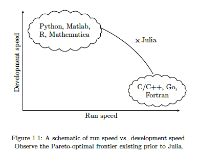
There are lots of advantages to Julia, just like there are lots of advantages with the other languages. The following diagram illustrates one of the core advantages of Julia, it isn’t an interpreted language like R and Python, which means Julia will be significantly faster, yet still allows interactive development using Notebooks, just like R and Python. Julia was designed and build for data science and machine learning, and is designed for scale which makes it a good fit for MLOps. The list of advantages and differences can go on a bit and those are not the point of this post.
The remainder of this post will step through what is needed to get Julia working with an Oracle Database, and you have setup an IDE. Check out the Julia website for excellent installation instructions and selecting an IDE. If you coming from an R and/or Python background, using Jupyter Notebooks is a good option, and as you become more experienced there are a number of more advanced IDEs available for you to use. I’m assuming you have installed Julia.
If you have done a new install of Julia, make sure to add the install directory to the search PATH.
First Download load and install Oracle Instant Client. This is needed by the Julia packages to communicate with Oracle Database. After installing make sure to setup the following in your environment (environment variables and Path)
- ORACLE_HOME : points to where you installed Oracle Instant Client
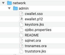
- TNS_ADMIN : points to the directory containing the wallet/tnsnames files. This will be a sub-directory in Oracle Instant Client directory, for example, it points to …/instantclient_19_8/network/admin
- PATH : include the Oracle Instant Client install directory in the PATH.
Next step is to setup the Oracle Client network files. As your DBA for the tnsnames.ora file or for the Wallet Zip file for your database. The Wallet Zip file is the most common approach. Unzip this Wallet file and copy the unzipped files to the TNS_ADMIN directory. See the second bullet point above to for this (…/instantclient_19_8/network/admin).
That’s all you need to do on the Oracle setup. I’m assuming you have a username and password for the Oracle Database you will be using.
Now we can setup Julia to use the Oracle Instant Client software. It is important you have setup those environment variables l’ve listed above.
There is an Oracle.jl package, developed by Felipe Noronha, which runs on top of Oracle Instant Client. To install this, load the Pkg package then then add the Oracle package. The following shows these commands and part of the output from the installation.
julia> using Pkg

julia> Pkg.add("Oracle")
Updating registry at `~/.julia/registries/General`
######################################################################## 100.0%
Resolving package versions...
Installed Reexport ──────────────────── v1.0.0
Installed libsodium_jll ─────────────── v1.0.18+1
Installed Compat ────────────────────── v3.25.0
Installed OrderedCollections ────────── v1.3.3
Installed WebSockets ────────────────── v1.5.9
Installed JuliaInterpreter ──────────── v0.8.8
Installed DataStructures ────────────── v0.18.9
Installed DataAPI ───────────────────── v1.5.1
Installed Requires ──────────────────── v1.1.2
Installed DataValueInterfaces ───────── v1.0.0
Installed Parsers ───────────────────── v1.0.15
Installed FlameGraphs ───────────────── v0.2.5
Installed URIs ──────────────────────── v1.2.0
Installed Colors ────────────────────── v0.12.6
Installed Oracle ────────────────────── v0.2.0
...
...
...
[7240a794] + Oracle v0.2.0
[bac558e1] ↑ OrderedCollections v1.3.2 ⇒ v1.3.3
[69de0a69] ↑ Parsers v1.0.12 ⇒ v1.0.15
[189a3867] ↑ Reexport v0.2.0 ⇒ v1.0.0
[ae029012] ↑ Requires v1.1.1 ⇒ v1.1.2
[3783bdb8] + TableTraits v1.0.0
[bd369af6] + Tables v1.3.2
[0796e94c] ↑ Tokenize v0.5.8 ⇒ v0.5.13
[5c2747f8] + URIs v1.2.0
[104b5d7c] ↑ WebSockets v1.5.2 ⇒ v1.5.9
[8f1865be] ↑ ZeroMQ_jll v4.3.2+5 ⇒ v4.3.2+6
[a9144af2] + libsodium_jll v1.0.18+1
Building Oracle → `~/.julia/packages/Oracle/CEOWz/deps/build.log`

julia>
You are now ready to load this Oracle package and use it to connect to an Oracle Database. Setting up a connection is really simple and in the following example I’m connecting to an ATP Database on Oracle Free Tier. The following sets up some variables, creates a connection, prints a statement and connection information and then closes the connection.
import Oracle

username="oml_user"
password="xxxxxxxxxxx"
dbname="yyyyyyyyyyyy"

conn = Oracle.Connection(username, password, dbname)

println("Connected")
println(conn)

Oracle.close(conn)
Job done 🙂
There is little additional connection information available. To test the connection a bit more let’s list what tables I have in my test/demo schema/user.
import Oracle

username="oml_user"
password="xxxxxxxxxxx"
dbname="yyyyyyyyyyyy"

conn = Oracle.Connection(username, password, dbname)

println("Tables")
println("--------------------")

Oracle.query(conn, "SELECT table_name FROM user_tables") do cursor
    for row in cursor
    # row values can be accessed using column name or position
        println( row["TABLE_NAME"] ) # same as row[1]
    end
end

println("")
println("...the end...")

Oracle.close(conn)
If you come from a Python background the syntax is familiar which makes the move other to Julia an easier task.
One other difference is, running the above code does seem to run a lot quicker in Julia. I haven’t measured it and the difference is less than a second but it is noticeable. For me, the above code generate the following output,
Tables
--------------------
WINE
BANK_ADDITIONAL_FULL
MINING_DATA_BUILD_V

...the end...
I’ll have additional posts looking are difference aspects and commands for working with and processing data in an Oracle Database.
Collection of Oracle 21c posts on new Machine Learning and Statistical functions
Oracle 21c was officially released a few days about and this post contains links to some blog posts I’ve written on new machine learning and statistical functions in the new Oracle 21c.
- Adam Optimization Solver for Neural Network Algorithm
- MSET-SPRT Algorithm
- XGBoost Algorithm
- Measuring SKEWNESS Function
- Measuring tailedness of data with KURTOSIS Function
I also have posts on new OML4Py and AutoML too, and I’ll have a different set of posts for those, so look out them.
Also check out my previous blog post that covers new machine learning feature introduced in Oracle 19c.
Measuring Kurtosis of Data in Oracle (21c)
Kurtosis is a new analytics function in Oracle 21c (20c) and is one of a set of commonly used statistical functions used to evaluate data to see and understand the behavior of the data.
[See my previous post where I give examples of the new Skewness functions]
Kurtosis is the measurement of the tails of the data distribution and its comparison with that of normal distribution. The Kurtosis of the normal distribution is said to be 3. To make interpenetrating results easier (a Zero) kurtosis measure for gaussian/normal distribution by subtracting 3 from its value, this is called Excess Kurtosis. Kurtosis can be used to describe the height or the breath of the distributions, when compared to a normal distributions, although this is not theoretically correct, it gives a simpler explanation and visualization of it. The following diagram gives an example of a normal distribution, a plot of Positive Kurtosis and Negative Kurtosis.

Prior to the new Kurtosis SQL functions (KURTOSIS_POP and KURTOSIS_SAMP), you had to calculate the Kurtosis value manually using something like the following SQL. These use the same data and attributes set used for the Skewness examples.
select avg(KV) K_value
from (select power((age - avg(age) over ())/stddev(age) over (), 4) KV
      from cust_data)
union all
select avg(KV) K_value
from (select power((duration - avg(duration) over ())/stddev(duration) over (), 4) KV
      from cust_data);

K_value
------------------------------------------
3.79088571963003808388287765230733611415
23.24420570926391173498028369605428048285
These don’t include the subtraction of 3 to give a zero kurtosis, and these values can be compared to the data distribution charts shown in the Skewness post.
Now with the new Kurtosis functions it simplifies the tasks of getting these values.
SELECT kurtosis_pop(age), kurtosis_samp(age)
FROM bank_additional
union all
SELECT kurtosis_pop(duration), kurtosis_samp(duration)
FROM bank_additional;

KURTOSIS_POP         KURTOSIS_SAMP
------------------   -----------------------------------------
 0.791069803527387    0.79131153115443467194451597661213420763
20.245334438614832   20.24793801497878942299945619307526969226
As you can see the Kurtosis function have the subtraction include.
As with the Skewness functions, the SAMP version works on a sample of the data values and as the number inputs increases, and differences between the POP and SAMP will reduce.
Enhanced Window Clause functionality in Oracle 21c (20c)
Updated: Changed 20c to Oracle 21c, as Oracle 20c Database never really existed 🙂
The Oracle Database has had advanced analytical functions for some time now and with each release we get to have some new additions or some enhancements to existing functionality.
One new enhancement, available and documented in 21c (not yet released at time of writing this), is changing in the way the Window Clause can be defined for analytic functions. Oracle 21c is available on Oracle Cloud as a pre-release for evaluation purposes (but it won’t be available for much longer!). The examples shown below are based on using this 21c pre-release of the database.
NOTE: At this point, no one really knows when or if 20c will be released. I’m sure all the documented 20c new features will be rolled into 21c, whenever that will be released.
Before giving some examples of the new Window Clause functionality, lets have a quick recap on how we could use it up to now (up to 19c database). Here is a simple example of windowing the data by creating partitions based on the distinct values in DEPTNO column
select deptno,
       ename,
       job,
       salary,
       avg (salary) over (partition by DEPTNO) avg_sal
from employee
order by deptno;

Here we get to see the average salary being calculated for each window partition and being reset for the next windwo partition.
The SQL:2011 standard support the defining of the Window clause in the query block, after defining the list tables for the query. This allows us to define the window clause one and then reference this for analytic function that need it. The following example illustrate this. I’ve take the able query and altered it to have the newer syntax. I’ve highlighted the new or changed code in blue. In the analytic function, the w1 refers to the Window clause defined later, and is more in keeping with how a query is logically processed.
select deptno,
       ename,
       sal,
       sum(sal) over (w1) sum_sal
from emp
   window w1 as (partition by deptno);
As you would expect we get the same results returned.
This newer syntax is particularly useful when we have many more analytic function in our queries, and some of these are using slightly different windowing. To me it makes it easier to read and to make edits, allowing an edit to be preformed once instead of for each analytic function, and avoids any errors. But making it easier to read and understand is by far the greatest benefit. Here is another example which uses different window clauses using the previous syntax.
SELECT deptno,
       ename,
       sal,
       AVG(sal) OVER (PARTITION BY deptno ORDER BY sal) AS avg_dept_sal,
       AVG(sal) OVER (PARTITION BY deptno ) AS avg_dept_sal2,
       SUM(sal) OVER (PARTITION BY deptno ORDER BY sal desc) AS sum_dept_sal
FROM emp;
Using the newer syntax this gets transformed into the following.
SELECT deptno,
       ename,
       sal,
       AVG(sal) OVER (w1) AS avg_dept_sal,
       AVG(sal) OVER (w2) AS avg_dept_sal2,
       SUM(sal) OVER (w2) AS avg_dept_sal
FROM emp
   window w1 as (PARTITION BY deptno ORDER BY sal),
          w2 as (PARTITION BY deptno),
          w3 as (PARTITION BY deptno ORDER BY sal desc);
- ← Previous
- 1
- 2
- 3
- …
- 5
- Next →

You must be logged in to post a comment.