
Oracle
Enhanced Window Clause functionality in Oracle 21c (20c)
Updated: Changed 20c to Oracle 21c, as Oracle 20c Database never really existed 🙂
The Oracle Database has had advanced analytical functions for some time now and with each release we get to have some new additions or some enhancements to existing functionality.
One new enhancement, available and documented in 21c (not yet released at time of writing this), is changing in the way the Window Clause can be defined for analytic functions. Oracle 21c is available on Oracle Cloud as a pre-release for evaluation purposes (but it won’t be available for much longer!). The examples shown below are based on using this 21c pre-release of the database.
NOTE: At this point, no one really knows when or if 20c will be released. I’m sure all the documented 20c new features will be rolled into 21c, whenever that will be released.
Before giving some examples of the new Window Clause functionality, lets have a quick recap on how we could use it up to now (up to 19c database). Here is a simple example of windowing the data by creating partitions based on the distinct values in DEPTNO column
select deptno,
       ename,
       job,
       salary,
       avg (salary) over (partition by DEPTNO) avg_sal
from employee
order by deptno;

Here we get to see the average salary being calculated for each window partition and being reset for the next windwo partition.
The SQL:2011 standard support the defining of the Window clause in the query block, after defining the list tables for the query. This allows us to define the window clause one and then reference this for analytic function that need it. The following example illustrate this. I’ve take the able query and altered it to have the newer syntax. I’ve highlighted the new or changed code in blue. In the analytic function, the w1 refers to the Window clause defined later, and is more in keeping with how a query is logically processed.
select deptno,
       ename,
       sal,
       sum(sal) over (w1) sum_sal
from emp
   window w1 as (partition by deptno);
As you would expect we get the same results returned.
This newer syntax is particularly useful when we have many more analytic function in our queries, and some of these are using slightly different windowing. To me it makes it easier to read and to make edits, allowing an edit to be preformed once instead of for each analytic function, and avoids any errors. But making it easier to read and understand is by far the greatest benefit. Here is another example which uses different window clauses using the previous syntax.
SELECT deptno,
       ename,
       sal,
       AVG(sal) OVER (PARTITION BY deptno ORDER BY sal) AS avg_dept_sal,
       AVG(sal) OVER (PARTITION BY deptno ) AS avg_dept_sal2,
       SUM(sal) OVER (PARTITION BY deptno ORDER BY sal desc) AS sum_dept_sal
FROM emp;
Using the newer syntax this gets transformed into the following.
SELECT deptno,
       ename,
       sal,
       AVG(sal) OVER (w1) AS avg_dept_sal,
       AVG(sal) OVER (w2) AS avg_dept_sal2,
       SUM(sal) OVER (w2) AS avg_dept_sal
FROM emp
   window w1 as (PARTITION BY deptno ORDER BY sal),
          w2 as (PARTITION BY deptno),
          w3 as (PARTITION BY deptno ORDER BY sal desc);
Exploring Database trends using Python pytrends (Google Trends)
A little word of warning before you read the rest of this post. The examples shown below are just examples of what is possible. It isn’t very scientific or rigorous, so don’t come complaining if what is shown doesn’t match your knowledge and other insights. This is just a little fun to see what is possible. Yes a more rigorous scientific study is needed, and some attempts at this can be seen at DB-Engines.com. Less scientific are examples shown at TOPDB Top Database index and that isn’t meant to be very scientific.
After all of that, here we go 🙂
pytrends is a library providing an API to Google Trends using Python. The following examples show some ways you can use this library and the focus area I’ll be using is Databases. Many of you are already familiar with using Google Trends, and if this isn’t something you have looked at before then I’d encourage you to go have a look at their website and to give it a try. You don’t need to run Python to use it. For example, here is a quick example taken from the Google Trends website. Here are a couple of screen shots from Google Trends, comparing Relational Database to NoSQL Database. The information presented is based on what searches have been performed over the past 12 months. Some of the information is kind of interesting when you look at the related queries and also the distribution of countries.


To install pytrends use the pip command
pip3 install pytrends
As usual it will change the various pendent libraries and will update where necessary. In my particular case, the only library it updated was the version of pandas.
You do need to be careful of how many searches you perform as you may be limited due to Google rate limits. You can get around this by using a proxy and there is an example on the pytrends PyPi website on how to get around this.
The following code illustrates how to import and setup an initial request. The pandas library is also loaded as the data returned by pytrends API into a pandas dataframe. This will make it ease to format and explore the data.
import pandas as pd
from pytrends.request import TrendReq

pytrends = TrendReq()
The pytrends API has about nine methods. For my example I’ll be using the following:
- Interest Over Time: returns historical, indexed data for when the keyword was searched most as shown on Google Trends’ Interest Over Time section.
- Interest by Region: returns data for where the keyword is most searched as shown on Google Trends’ Interest by Region section.
- Related Queries: returns data for the related keywords to a provided keyword shown on Google Trends’ Related Queries section.
- Suggestions: returns a list of additional suggested keywords that can be used to refine a trend search.
Let’s now explore these APIs using the Databases as the main topic of investigation and examining some of the different products. I’ve used the db-engines.com website to select the top 5 databases (as per date of this blog post). These were:
- Oracle
- MySQL
- SQL Server
- PostgreSQL
- MongoDB
I will use this list to look for number of searches and other related information. First thing is to import the necessary libraries and create the connection to Google Trends.
import pandas as pd
from pytrends.request import TrendReq

pytrends = TrendReq()
Next setup the payload and keep the timeframe for searches to the past 12 months only.
search_list = ["Oracle", "MySQL", "SQL Server", "PostgreSQL", "MongoDB"] #max of 5 values allowed
pytrends.build_payload(search_list, timeframe='today 12-m')
We can now look at the the interest over time method to see the number of searches, based on a ranking where 100 is the most popular.
df_ot = pd.DataFrame(pytrends.interest_over_time()).drop(columns='isPartial')
df_ot

and to see a breakdown of these number on an hourly bases you can use the get_historical_interest method.
pytrends.get_historical_interest(search_list)
Let’s move on to exploring the level of interest/searches by country. The following retrieves this information, ordered by Oracle (in decending order) and then select the top 20 countries. Here we can see the relative number of searches per country. Note these doe not necessarily related to the countries with the largest number of searches
df_ibr = pytrends.interest_by_region(resolution='COUNTRY') # CITY, COUNTRY or REGION
df_ibr.sort_values('Oracle', ascending=False).head(20)

Visualizing data is always a good thing to do as we can see a patterns and differences in the data in a clearer way. The following takes the above query and creates a stacked bar chart.
import matplotlib
from matplotlib import pyplot as plt

df2 = df_ibr.sort_values('Oracle', ascending=False).head(20)

df2.reset_index().plot(x='geoName', y=['Oracle', 'MySQL', 'SQL Server', 'PostgreSQL', 'MongoDB'], kind ='bar', stacked=True, title="Searches by Country")

plt.rcParams["figure.figsize"] = [20, 8]
plt.xlabel("Country")
plt.ylabel("Ranking")

We can delve into the data more, by focusing on one particular country and examine the google searches by city or region. The following looks at the data from USA and gives the rankings for the various states.
pytrends.build_payload(search_list, geo='US')
df_ibr = pytrends.interest_by_region(resolution='COUNTRY', inc_low_vol=True)
df_ibr.sort_values('Oracle', ascending=False).head(20)

df2.reset_index().plot(x='geoName', y=['Oracle', 'MySQL', 'SQL Server', 'PostgreSQL', 'MongoDB'], kind ='bar', stacked=True, title="test")
plt.rcParams["figure.figsize"] = [20, 8]

plt.title("Searches for USA")
plt.xlabel("State")
plt.ylabel("Ranking")


We can find the top related queries and and top queries including the names of each database.
search_list = ["Oracle", "MySQL", "SQL Server", "PostgreSQL", "MongoDB"] #max of 5 values allowed
pytrends.build_payload(search_list, timeframe='today 12-m')

rq = pytrends.related_queries()
rq.values()

#display rising terms
rq.get('Oracle').get('rising')
We can see the top related rising queries for Oracle are about tik tok. No real surprise there!

and the top queries for Oracle included:
rq.get('Oracle').get('top')

This was an interesting exercise to do. I didn’t show all the results, but when you explore the other databases in the list and see the results from those, and then compare them across the five databases you get to see some interesting patterns.
Principal Component Analysis (PCA) in Oracle
Principal Component Analysis (PCA), is a statistical process used for feature or dimensionality reduction in data science and machine learning projects. It summarizes the features of a large data set into a smaller set of features by projecting each data point onto only the first few principal components to obtain lower-dimensional data while preserving as much of the data’s variation as possible. There are lots of resources that goes into the mathematics behind this approach. I’m not going to go into that detail here and a quick internet search will get you what you need.
PCA can be used to discover important features from large data sets (large as in having a large number of features), while preserving as much information as possible.
Oracle has implemented PCA using Sigular Value Decomposition (SVD) on the covariance and correlations between variables, for feature extraction/reduction. PCA is closely related to SVD. PCA computes a set of orthonormal bases (principal components) that are ranked by their corresponding explained variance. The main difference between SVD and PCA is that the PCA projection is not scaled by the singular values. The extracted features are transformed features consisting of linear combinations of the original features.
When machine learning is performed on this reduced set of transformed features, it can completed with less resources and time, while still maintaining accuracy.
Algorithm Name in Oracle using
Mining Model Function = FEATURE_EXTRACTION
Algorithm = ALGO_SINGULAR_VALUE_DECOMP
(Hyper)-Parameters for algorithms
- SVDS_U_MATRIX_OUTPUT : SVDS_U_MATRIX_ENABLE or SVDS_U_MATRIX_DISABLE
- SVDS_SCORING_MODE : SVDS_SCORING_SVD or SVDS_SCORING_PCA
- SVDS_SOLVER : possible values include SVDS_SOLVER_TSSVD, SVDS_SOLVER_TSEIGEN, SVDS_SOLVER_SSVD, SVDS_SOLVER_STEIGEN
- SVDS_TOLERANCE : range of 0…1
- SVDS_RANDOM_SEED : range of 0…4294967296 (!)
- SVDS_OVER_SAMPLING : range of 1…5000
- SVDS_POWER_ITERATIONS : Default value 2, with possible range of 0…20
Let’s work through an example using the MINING_DATA_BUILD_V data set that comes with Oracle Data Miner.
First step is to define the parameter settings for the algorithm. No data preparation is needed as the algorithm takes care of this. This means you can disable the Automatic Data Preparation (ADP).
-- create the parameter table
CREATE TABLE svd_settings (
setting_name VARCHAR2(30),
setting_value VARCHAR2(4000));

-- define the settings for SVD algorithm
BEGIN
   INSERT INTO svd_settings (setting_name, setting_value)
   VALUES (dbms_data_mining.algo_name, dbms_data_mining.algo_singular_value_decomp);

   -- turn OFF ADP
   INSERT INTO svd_settings (setting_name, setting_value)
   VALUES (dbms_data_mining.prep_auto, dbms_data_mining.prep_auto_off);

   -- set PCA scoring mode
   INSERT INTO svd_settings (setting_name, setting_value)
   VALUES (dbms_data_mining.svds_scoring_mode, dbms_data_mining.svds_scoring_pca);

   INSERT INTO svd_settings (setting_name, setting_value)
   VALUES (dbms_data_mining.prep_shift_2dnum, dbms_data_mining.prep_shift_mean);

   INSERT INTO svd_settings (setting_name, setting_value)
   VALUES (dbms_data_mining.prep_scale_2dnum, dbms_data_mining.prep_scale_stddev);
END;
/
You are now ready to create the model.
BEGIN
   DBMS_DATA_MINING.CREATE_MODEL(
      model_name          => 'SVD_MODEL',
      mining_function     => dbms_data_mining.feature_extraction,
      data_table_name     => 'mining_data_build_v',
      case_id_column_name => 'CUST_ID',
      settings_table_name => 'svd_settings');
END;
When created you can use the mining model data dictionary views to explore the model and to explore the specifics of the model and the various MxN matrix created using the model specific views. These include:
- DM$VESVD_Model : Singular Value Decomposition S Matrix
- DM$VGSVD_Model : Global Name-Value Pairs
- DM$VNSVD_Model : Normalization and Missing Value Handling
- DM$VSSVD_Model : Computed Settings
- DM$VUSVD_Model : Singular Value Decomposition U Matrix
- DM$VVSVD_Model : Singular Value Decomposition V Matrix
- DM$VWSVD_Model : Model Build Alerts
Where the S, V and U matrix contain:
- U matrix : consists of a set of ‘left’ orthonormal bases
- S matrix : is a diagonal matrix
- V matrix : consists of set of ‘right’ orthonormal bases
These can be explored using the following
-- S matrix
select feature_id, VALUE, variance, pct_cum_variance
from DM$VESVD_MODEL;

-- V matrix
select feature_id, attribute_name, value
from DM$VVSVD_MODEL
order by feature_id, attribute_name;

-- U matrix
select feature_id, attribute_name, value
from DM$VVSVD_MODEL
order by feature_id, attribute_name;
To determine the projections to be used for visualizations we can use the FEATURE_VALUES function.
select FEATURE_VALUE(svd_sh_sample, 1 USING *) proj1,
       FEATURE_VALUE(svd_sh_sample, 2 USING *) proj2
from   mining_data_build_v
where  cust_id <= 101510
order by 1, 2;
Other algorithms available in Oracle for feature extraction and reduction include:
- Non-Negative Matrix Factorization (NMF)
- Explicit Semantic Analysis (ESA)
- Minimum Description Length (MDL) – this is really feature selection rather than feature extraction
ONNX for exchanging Machine Learning Models
When working on build predictive application using machine learning algorithms, you will probably be working with such languages as Python, R, PyTorch, TensorFlow, and lots of other frameworks. One of the challenges we face is taking these machine learning models from our test/lab environment and putting into production them. By this I mean integrating them with our production systems to allow real-time use of these ML models. This is not a topic that is discussed very often. Many of the most common languages and frameworks are very easy to use for machine learning, but running them in production can be slow. This can lead to lots of problems and can regularly label machine learning projects as a failure. None of use want that. Sometime people look are re-coding all the machine learning models in other languages such as C or Java or Julia, as these are noted for the high speed and scalability in production environments. (Remember many of the common ML languages and frameworks are actually developed using C and Java.)
To remove the need to recode your models, many of the languages, frameworks and tools have opened to the ability to allow model interchange. This approach allows you to use the tools that work best for you, in your environment and your company, to develop, test and evaluate machine learning models. These can then be packaged up and shared with other languages, frameworks or tools suitable for production environments, eliminating or significantly reducing the need for large coding projects and allows for quicker time to deployment.
There are many machine learning model interchange frameworks available. Historically PMML was popular but with the rise of other machine learning and deep learning algorithms, it seems to have lost the popularity contest. One of the more popular machine learning interchange frameworks is called ONNX. This has been growing in popularity with a wide body of languages, tools and vendors.

ONNX stands for the Open Neural Network eXchange and is designed to allow developers to easily move between different machine learning and deep learning frameworks. This allows the easy migration from research and model development environments, to other environments more suited to deployment, allowing for faster scoring of data. ONNX allows for the migration of the model with the minimum of recoding. ONNX generates or provides for an extensible computation dataflow graph model, with built-in operators and data types focused on interencing.
To use ONNX with Python install the library:
pip3 install onnx-mxnetThe following is an extract of sample code generating a model, converting it to ONNX format and saving it to file.
#train a model
#load sklearn
from sklearn.datasets import load_iris
from sklearn.model_selection import train_test_split
from sklearn.ensemble import RandomForestClassifier

#load the IRIS sample data set
iris = load_iris()
X, y = iris.data, iris.target
#create the train and test data sets
X_train, X_test, y_train, y_test = train_test_split(X, y)
#define and create Random Forest data set
rf = RandomForestClassifier()
rf.fit(X_train, y_train)

#convert into ONNX format & save to file
from skl2onnx import convert_sklearn
from skl2onnx.common.data_types import FloatTensorType
initial_type = [('float_input', FloatTensorType([None, 4]))]
#covert to ONNX
onx = convert_sklearn(rf, initial_types=initial_type)
#save to file
with open("rf_iris.onnx", "wb") as f:
    f.write(onx.SerializeToString())
The above example illustrates converting a sklearn model. For algorithms and models, converters exist and are available in the ONNX Github
Loading and Reading Binary files in Oracle Database using Python
Most Python example show how to load data into a database table. In this blog post I’ll show you how to load a binary file, for example a picture, into a table in an Oracle Autonomous Database (ATP or ADW) and how to read that same image back using Python.
Before we can do this, we need to setup a few things. These include,
Let’s use the following table
CREATE TABLE demo_blob (
   id     NUMBER PRIMARY KEY,
   image_txt   VARCHAR2(100),
   image   BLOB);
Now let’s get onto the fun bit of loading a image file into this table. The image I’m going to use is the cover of my Data Science book published by MIT Press.

I have this file saved in ‘…/MyBooks/DataScience/BookCover.jpg’.
#Read the binary file
with open (".../MyBooks/DataScience/BookCover.jpg", 'rb') as file:
    blob_file = file.read()

#Display some details of file
print('Length =', len(blob_file))
print('Printing first part of file')
print(blob_file[:50])
Now define the insert statement and setup a cursor to process the insert statement;
#define prepared statement
inst_blob = 'insert into demo_blob (id, image_txt, image) values (:1, :2, :3)'

#connection created using cx_Oracle - see links earlier in post
cur = con.cursor()
Now insert the data and the binary file.
#setup values for attributes
idNum = 1
imageText = 'Demo inserting Blob file'
#insert data into table
cur.execute(inst_blob, (idNum, imageText, blob_file))

#close and finish
cur.close() #close the cursor
con.close() #close the database connection
The image is now saved in the database table. You can use Python to retrieve it or use other tools to view the image.
For example using SQL Developer, query the table and in the results window double click on the blob value. A window pops open and you can view on the image from there by clicking on the check box.
Now that we have the image loads into an Oracle Database the next step is the Python code to read and display the image.
#define prepared statement
qry_blog = 'select id, image_txt, image from demo_blob where id = :1'

#connection created using cx_Oracle - see links earlier in post
cur = con.cursor()
#setup values for attributes
idNum = 1
#execute the query
#query the data and blob data
connection.outputtypehandler = OutputTypeHandler
cur.execute(qry_blob, (idNum))
id, desc, blob_data = cur.fetchone()

#write the blob data to file
newFileName = '.../MyBooks/DataScience/DummyImage.jpg'
with open(newFileName, 'wb') as file:
   file.write(blob_data)
#close and finish
cur.close() #close the cursor
con.close() #close the database connection
Adam Solver for Neural Networks (OML) in Oracle 21c
Updated: Changed 20c to Oracle 21c, as Oracle 20c Database never really existed 🙂
The ability to create and use Neural Networks on business data has been available in Oracle Database since Oracle 18c (18c and 19c are just slightly extended versions of Oracle 12c). With each minor database release we get some small improvements and minor features added. I’ve written other blog posts about other 21c new machine learning features (see here, here and here).
With Oracle 21c they have added a new neural network solver. This is called Adam Solver and the original research was conducted by Diederik Kingma from OpenAI and Jimmy Ba from the University of Toronto and they presented they work at ICLR 2015. The name Adam is derived from ‘adaptive moment estimation‘. This algorithm, research and paper has gathered some attention in the research community over the past few years. Most of this has been focused on the benefits of using it.

But care is needed. As with most machine learning (and deep learning) algorithms, they work up to a point. They may be good on certain problems and input data sets, and then for others they may not be as good or as efficient at producing an optimal outcome. Although using this solver may be beneficial to your problem, using the concept of ‘No Free Lunch’, you will need to prove the solver is beneficial for your problem.
With Oracle Machine Learning there are two Optimization Solver available for the Neural Network algorithm. The default solver is call L-BFGS (Limited memory Broyden-Fletch-Goldfarb-Shanno). This is one of the most popular solvers in use in most algorithms. The is a limited version of BFGS, using less memory (hence the L in the name) This solver finds the descent direction and line search is used to find the appropriate step size. The solver searches for the optimal solution of the loss function to find the extreme value (maximum or minimum) of the loss (cost) function
The Adam Solver uses an extension to stochastic gradient descent. It uses the squared gradients to scale the learning rate and it takes advantage of momentum by using moving average of the gradient instead of gradient. This allows the solver to work quickly by seeing less data and can work well with larger data sets.
With Oracle Data Mining the Adam Solver has the following parameters.
- ADAM_ALPHA : Learning rate for solver. Default value is 0.001.
- ADAM_BATCH_ROWS : Number of rows per batch. Default value is 10,000
- ADAM_BETA1 : Exponential decay rate for 1st moment estimates. Default value is 0.9.
- ADAM_BETA2 : Exponential decay rate for the 2nd moment estimates. Default value is 0.99.
- ADAM_GRADIENT_TOLERANCE : Gradient infinity norm tolerance. Default value is 1E-9.
The parameters ADAM_ALPHA and ADAM_BATCH_ROWS can have an effect on the timing for the neural network algorithm to produce the model. Some exploration is needed to determine the optimal values for this parameters based on the size of the data set. For example having a larger value for ADAM_ALPHA results in a faster initial learning before the rates is updated. Small values than the default slows learning down during training.
To tell Oracle Machine Learning to use the Adam Solver the DMSSET_NN_SOLVER parameter needs to be set. The default setting for a neural network is DMSSET_NN_SOLVER_LGFGS. But to use the Adam solver set it to DMSSET_NN_SOLVER_ADAM.
The following is an example of setting the parameters for the Adam solver and creating a neural network.
BEGIN
   DELETE FROM BANKING_NNET_SETTINGS;

   INSERT INTO BANKING_NNET_SETTINGS (setting_name, setting_value)
   VALUES (dbms_data_mining.algo_name, dbms_data_mining.algo_neural_network);

   INSERT INTO BANKING_NNET_SETTINGS (setting_name, setting_value)
   VALUES (dbms_data_mining.prep_auto, dbms_data_mining.prep_auto_on);

   INSERT INTO BANKING_NNET_SETTINGS (setting_name, setting_value)
   VALUES (dbms_data_mining.nnet_nodes_per_layer, '20,10,6');

   INSERT INTO BANKING_NNET_SETTINGS (setting_name, setting_value)
   VALUES (dbms_data_mining.nnet_iterations, 10);

   INSERT INTO BANKING_NNET_SETTINGS (setting_name, setting_value)
   VALUES (dbms_data_mining.NNET_SOLVER, 'NNET_SOLVER_ADAM');
END;

The addition of the last parameter overrides the default solver for building a neural network model.
To build the model we can use the following.
DECLARE
   v_start_time TIMESTAMP;
BEGIN
   begin DBMS_DATA_MINING.DROP_MODEL('BANKING_NNET_72K_1'); exception when others then null; end;

   v_start_time := current_timestamp;
   DBMS_DATA_MINING.CREATE_MODEL(
      model_name.         => 'BANKING_NNET_72K_1',
      mining_function     => dbms_data_mining.classification,
      data_table_name     => 'BANKING_72K',
      case_id_column_name => 'ID',
      target_column_name  => 'TARGET',
      settings_table_name => 'BANKING_NNET_SETTINGS');

   dbms_output.put_line('Time take to create model = ' || to_char(extract(second from (current_timestamp-v_start_time))) || ' seconds.');
END;
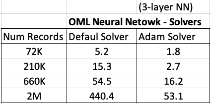
For me on my Oracle 20c Preview Database, this takes 1.8 seconds to run and create the neural network model ob a data set of 72,000 records.
Using the default solver, the model is created in 5.2 seconds. With using a small data set of 72,000 records, we can see the impact of using an Adam Solver for creating a neural network model.
These timings and the timings shown below (in seconds) are based on the Oracle 20c Preview Database, using a minimum VM sizing and specification available.
Partitioned Models – Oracle Machine Learning (OML)
Building machine learning models can be a relatively trivial task. But getting to that point and understanding what to do next can be challenging. Yes the task of creating a model is simple and usually takes a few line of code. This is what is shown in most examples. But when you try to apply to real world problems we are faced with other challenges. Some of which include volume of data is larger, building efficient ML pipelines is challenging, time to create models gets longer, applying models to new data in real-time takes longer (not possible in real-time), etc. Yes these are typically challenges and most of these can be easily overcome.
When building ML solutions for real-world problem you will be faced with building (and deploying) many 10s or 100s of ML models. Why are so many models needed? Almost every example we see for ML takes the entire data set and build a model on that data. When you think about it, not everyone in the data set can be considered in the same grouping (similar characteristics). If we were to build a model on the data set and apply it to new data, we will get a generic prediction. A prediction comparing the new data item (new customer, purchase, etc) with everyone else in the data population. Maybe this is why so many ML project fail as they are building generic solution that performs badly when run on new (and evolving) data.
To overcome this we start to look at the different groups of data in the data set. Can the data set be divided into a number of different parts based on some characteristics. If we could do this and build a separate model on each group (or cluster), then we would have ML models that would be more accurate with their predictions. This is where we will end up creating 10s or 100s of models. As you can imagine the work involved in doing this with be LOTs. Then think about all the coding needed to manage all of this. What about the complexity of all the code needed for making the predictions on new data.
Yes all of this gets complex very, very quickly!
Ideally we want a separate model for each group
But how can you do that efficiently? is it possible?
When working with Oracle Machine Learning, you can use a feature called partitioned models. Partitioned Models are designed to handle this type of problem. They are designed to:
- make the building of models simple
- scales as the data and number of partitions increase
- includes all the steps part of the ML pipeline (all the data prep, transformations, etc)
- make predicting new data using the ML model simple
- make the deployment of the ML model easy
- make the MLOps process simple
- make the use of ML model easy to use by all developers no matter the programming language
- make the ML model build and ML model scoring quick and with better, more accurate predictions.

Let us work through an example. In this example lets start by creating a Random Forest ML model using the entire data set. The following code shows setting up the Parameters settings table. The second code segment creates the Random Forest ML model. The training data set being used in this example contains 72,000 records.
BEGIN
  DELETE FROM BANKING_RF_SETTINGS;

  INSERT INTO banking_RF_settings (setting_name, setting_value)
  VALUES (dbms_data_mining.algo_name, dbms_data_mining.algo_random_forest);

  INSERT INTO banking_RF_settings (setting_name, setting_value)
  VALUES (dbms_data_mining.prep_auto, dbms_data_mining.prep_auto_on);

 COMMIT;
END;
/

-- Create the ML model
DECLARE
   v_start_time  TIMESTAMP;
BEGIN
   DBMS_DATA_MINING.DROP_MODEL('BANKING_RF_72K_1');

   v_start_time := current_timestamp;

   DBMS_DATA_MINING.CREATE_MODEL(
      model_name          => 'BANKING_RF_72K_1',
      mining_function     => dbms_data_mining.classification,
      data_table_name     => 'BANKING_72K',
      case_id_column_name => 'ID',
      target_column_name  => 'TARGET',
      settings_table_name => 'BANKING_RF_SETTINGS');

   dbms_output.put_line('Time take to create model = ' || to_char(extract(second from (current_timestamp-v_start_time))) || ' seconds.');
END;
/
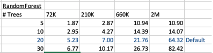
This is the basic setup and the following table illustrates how long the CREATE_MODEL function takes to run for different sizes of training datasets and with different number of trees per model. The default number of trees is 20.
To run this model against new data we could use something like the following SQL query.
SELECT cust_id, target,
       prediction(BANKING_RF_72K_1 USING *)  predicted_value,
       prediction_probability(BANKING_RF_72K_1 USING *) probability
FROM   bank_test_v;
This is simple and straight forward to use.
For the 72,000 records it takes just approx 5.23 seconds to create the model, which includes creating 20 Decision Trees. As mentioned earlier, this will be a generic model covering the entire data set.
To create a partitioned model, we can add new parameter which lists the attributes to use to partition the data set. For example, if the partition attribute is MARITAL, we see it has four different values. This means when this attribute is used as the partition attribute, Oracle Machine Learning will create four separate sub Random Forest models all until the one umbrella model. This means the above SQL query to run the model, does not change and the correct sub model will be selected to run on the data based on the value of MARITAL attribute.
To create this partitioned model you need to add the following to the settings table.
BEGIN
  DELETE FROM BANKING_RF_SETTINGS;

  INSERT INTO banking_RF_settings (setting_name, setting_value)
  VALUES (dbms_data_mining.algo_name, dbms_data_mining.algo_random_forest);

  INSERT INTO banking_RF_settings (setting_name, setting_value)
  VALUES (dbms_data_mining.prep_auto, dbms_data_mining.prep_auto_on);

  INSERT INTO banking_RF_settings (setting_name, setting_value)
  VALUES (dbms_data_mining.odms_partition_columns, 'MARITAL’);

COMMIT;
END;
/
The code to create the model remains the same!
The code to call and use the model remains the same!
This keeps everything very simple and very easy to use.
When I ran the CREATE_MODEL code for the partitioned model, it took approx 8.3 seconds to run. Yes it took slightly longer than the previous example, but this time it is creating four models instead of one. This is still very quick!
What if I wanted to add more attributes to the partition key? Yes you can do that. The more attributes you add, the more sub-models will be be created.
For example, if I was to add JOB attribute to the partition key list. I will now get 48 sub-models (with 20 Decision Trees each) being created. The JOB attribute has 12 distinct values, multiplied by the 4 values for MARITAL, gives us 48 models.
INSERT INTO banking_RF_settings (setting_name, setting_value)
VALUES (dbms_data_mining.odms_partition_columns, 'MARITAL,JOB');
How long does this take the CREATE_MODEL code to run? approx 37 seconds!
Again that is quick!
Again remember the code to create the model and to run the model to predict on new data does not change. This means our applications using this ML model does not change. This shows us we can very easily increase the predictive accuracy of our models with only adding one additional model, and by improving this accuracy by adding more attributes to the partition key.
But you do need to be careful with what attributes to include in the partition key. If the attributes have a very high number of distinct values, will result in 100s, or 1000s of sub models being created.
An important benefit of using partitioned models is when a new distinct value occurs in one of the partition key attributes. You code to create the parameters and models does not change. OML will automatically will pick this up and do all the work under the hood.
New Oracle Machine Learning Features in 19c and 20c
Here are links to blog posts and articles I’ve written about the new features of Oracle Machine Learning in 19c (and previous) and 20c.
I’ve given a presentation on these topics at ACES@Home and Yatra online conferences.
 Each of the following links will explain each of the algorithms, and gives demo code for you to try.
- RandomForest
https://oralytics.com/2020/06/24/randomforest-machine-learning-oracle-machine-learning-oml/
- Neural Networks
https://developer.oracle.com/databases/neural-network-machine-learning.html
- Time Series Forecasting
https://oralytics.com/2019/04/15/time-series-forecasting-in-oracle-part-1/
https://oralytics.com/2019/04/23/time-series-forecasting-in-oracle-part-2/
- XGBoost
https://oralytics.com/2020/04/27/xgboost-in-oracle-20c/
- Multivariate State Estimation Technique (MSET)
https://oralytics.com/2020/04/13/mset-multivariate-state-estimation-technique-in-oracle-20c/
- Partitioned Models
https://oralytics.com/2020/07/13/partitioned-models-oracle-machine-learning-oml/
- Parallel Model Creation
https://oralytics.com/2020/07/27/creating-oml-models-in-parallel/
GoLang: Links to blog posts – working with Oracle Database
This post is to serve as a link to my other blog posts on using GoLang and connecting to/working with data from an Oracle Database.
Connecting Go Lang to Oracle Database
The database driver/library got renamed. The following post goes through how to updated to new name.
GoLang: Oracle driver/library renamed to : godror
GoLang: Querying records from Oracle Database using goracle
GoLang: Inserting records into Oracle Database using goracle
Importance of setting Fetched Rows size for Database Query using Golang
GoLang – Consuming Oracle REST API from an Oracle Cloud Database)
This post will be updated with new GoLang posts.
XGBoost in Oracle 20c
 Updated: Changed 20c to Oracle 21c, as Oracle 20c Database never really existed 🙂
Another of the new machine learning algorithms in Oracle 21c Database is called XGBoost. Most people will have come across this algorithm due to its recent popularity with winners of Kaggle competitions and other similar events.
XGBoost is an open source software library providing a gradient boosting framework in most of the commonly used data science, machine learning and software development languages. It has it’s origins back in 2014, but the first official academic publication on the algorithm was published in 2016 by Tianqi Chen and Carlos Guestrin, from the University of Washington.
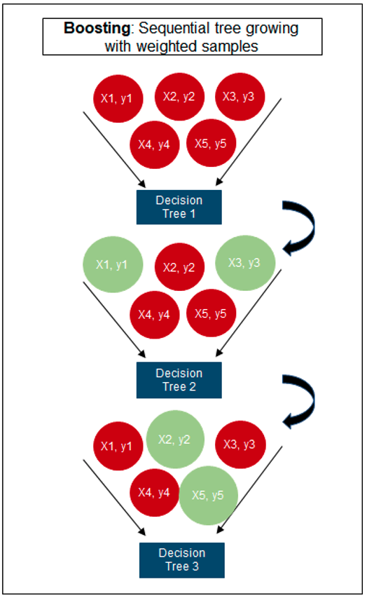
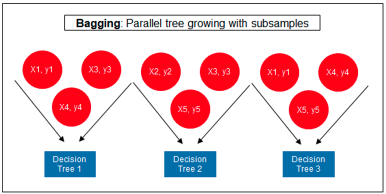
The algorithm builds upon the previous work on Decision Trees, Bagging, Random Forest, Boosting and Gradient Boosting. The benefits of using these various approaches are well know, researched, developed and proven over many years. XGBoost can be used for the typical use cases of Classification including classification, regression and ranking problems. Check out the original research paper for more details of the inner workings of the algorithm.
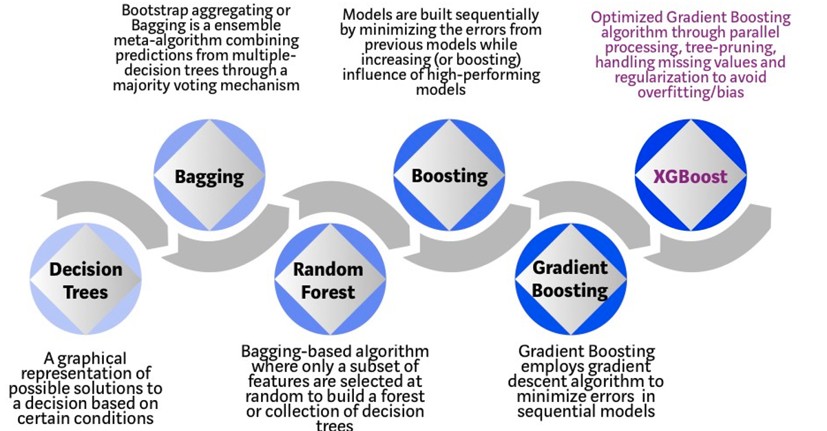
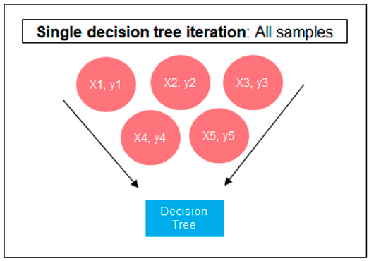
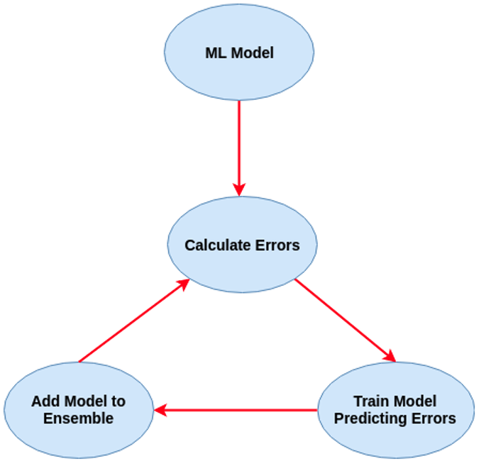 Regular machine learning models, like Decision Trees, simply train a single model using a training data set, and only this model is used for predictions. Although a Decision Tree is very simple to create (and very very quick to do so) its predictive power may not be as good as most other algorithms, despite providing model explainability. To overcome this limitation ensemble approaches can be used to create multiple Decision Trees and combines these for predictive purposes. Bagging is an approach where the predictions from multiple DT models are combined using majority voting. Building upon the bagging approach Random Forest uses different subsets of features and subsets of the training data, combining these in different ways to create a collection of DT models and presented as one model to the user. Boosting takes a more iterative approach to refining the models by building sequential models with each subsequent model is focused on minimizing the errors of the previous model. Gradient Boosting uses gradient descent algorithm to minimize errors in subsequent models. Finally with XGBoost builds upon these previous steps enabling parallel processing, tree pruning, missing data treatment, regularization and better cache, memory and hardware optimization. It’s commonly referred to as gradient boosting on steroids.
The following three images illustrates the differences between Decision Trees, Random Forest and XGBoost.
The XGBoost algorithm in Oracle 20c has over 40 different parameter settings, and with most scenarios the default settings with be fine for most scenarios. Only after creating a baseline model with the details will you look to explore making changes to these. Some of the typical settings include:
- Booster = gbtree
- #rounds for boosting = 10
- max_depth = 6
- num_parallel_tree = 1
- eval_metric = Classification error rate or RMSE for regression
As with most of the Oracle in-database machine learning algorithms, the setup and defining the parameters is really simple. Here is an example of minimum of parameter settings that needs to be defined.
BEGIN
   -- delete previous setttings
   DELETE FROM banking_xgb_settings;

   INSERT INTO BANKING_XGB_SETTINGS (setting_name, setting_value)
   VALUES (dbms_data_mining.algo_name, dbms_data_mining.algo_xgboost);

   -- For 0/1 target, choose binary:logistic as the objective.
   INSERT INTO BANKING_XGB_SETTINGS (setting_name, setting_value)
   VALUES (dbms_data_mining.xgboost_objective, 'binary:logistic’);

   commit;
END;
To create an XGBoost model run the following.


BEGIN
   DBMS_DATA_MINING.CREATE_MODEL (
      model_name          => 'BANKING_XGB_MODEL',
      mining_function     => dbms_data_mining.classification,
      data_table_name     => 'BANKING_72K',
      case_id_column_name => 'ID',
      target_column_name  => 'TARGET',
      settings_table_name => 'BANKING_XGB_SETTINGS');
END;
That’s all nice and simple, as it should be, and the new model can be called in the same manner as any of the other in-database machine learning models using functions like PREDICTION, PREDICTION_PROBABILITY, etc.
One of the interesting things I found when experimenting with XGBoost was the time it took to create the completed model. Using the default settings the following table gives the time taken, in seconds to create the model.
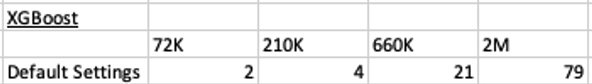
As you can see it is VERY quick even for large data sets and gives greater predictive accuracy.
MSET (Multivariate State Estimation Technique) in Oracle 20c
Updated: Changed 20c to Oracle 21c, as Oracle 20c Database never really existed 🙂
Oracle 21c Database comes with some new in-database Machine Learning algorithms.
The short name for one of these is called MSET or Multivariate State Estimation Technique. That’s the simple short name. The more complete name is Multivariate State Estimation Technique – Sequential Probability Ratio Test. That is a long name, and the reason is it consists of two algorithms. The first part looks at creating a model of the training data, and the second part looks at how new data is statistical different to the training data.
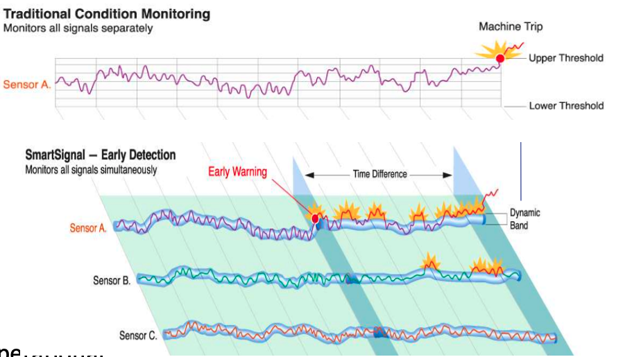
What are the use cases for this algorithm? This algorithm can be used for anomaly detection.

Anomaly Detection, using algorithms, is able identifying unexpected items or events in data that differ to the norm. It can be easy to perform some simple calculations and graphics to examine and present data to see if there are any patterns in the data set. When the data sets grow it is difficult for humans to identify anomalies and we need the help of algorithms.
The images shown here are easy to analyze to spot the anomalies and it can be relatively easy to build some automated processing to identify these. Most of these solutions can be considered AI (Artificial Intelligence) solutions as they mimic human behaviors to identify the anomalies, and these example don’t need deep learning, neural networks or anything like that.
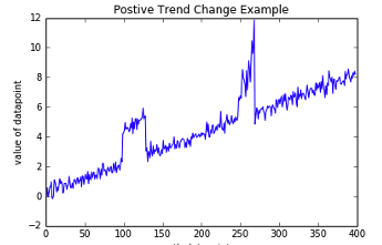
Other types of anomalies can be easily spotted in charts or graphics, such as the chart below.
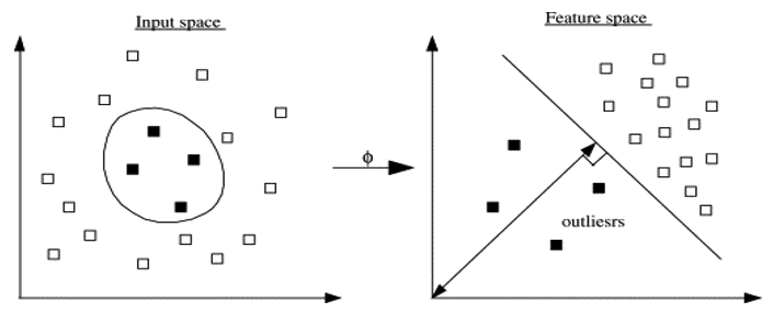 There are many different algorithms available for anomaly detection, and the Oracle Database already has an algorithm called the One-Class Support Vector Machine. This is a variant of the main Support Vector Machine (SVD) algorithm, which maps or transforms the data, using a Kernel function, into space such that the data belonging to the class values are transformed by different amounts. This creates a Hyperplane between the mapped/transformed values and hopefully gives a large margin between the mapped/transformed points. This is what makes SVD very accurate, although it does have some scaling limitations. For a One-Class SVD, a similar process is followed. The aim is for anomalous data to be mapped differently to common or non-anomalous data, as shown in the following diagram.
Getting back to the MSET algorithm. Remember it is a 2-part algorithm abbreviated to MSET. The first part is a non-linear, nonparametric anomaly detection algorithm that calibrates the expected behavior of a system based on historical data from the normal sequence of monitored signals. Using data in time series format (DATE, Value) the training data set contains data consisting of “normal” behavior of the data. The algorithm creates a model to represent this “normal”/stationary data/behavior. The second part of the algorithm compares new or live data and calculates the differences between the estimated and actual signal values (residuals). It uses Sequential Probability Ratio Test (SPRT) calculations to determine whether any of the signals have become degraded. As you can imagine the creation of the training data set is vital and may consist of many iterations before determining the optimal training data set to use.
MSET has its origins in computer hardware failures monitoring. Sun Microsystems have been were using it back in the late 1990’s-early 2000’s to monitor and detect for component failures in their servers. Since then MSET has been widely used in power generation plants, airplanes, space travel, Disney uses it for equipment failures, and in more recent times has been extensively used in IOT environments with the anomaly detection focused on signal anomalies.
How does MSET work in Oracle 21c?
An important point to note before we start is, you can use MSET on your typical business data and other data stored in the database. It isn’t just for sensor, IOT, etc data mentioned above and can be used in many different business scenarios.
The first step you need to do is to create the time series data. This can be easily done using a view, but a Very important component is the Time attribute needs to be a DATE format. Additional attributes can be numeric data and these will be used as input to the algorithm for model creation.
-- Create training data set for MSET
CREATE OR REPLACE VIEW mset_train_data
AS SELECT time_id,
          sum(quantity_sold) quantity,
          sum(amount_sold) amount
FROM (SELECT * FROM sh.sales WHERE time_id <= '30-DEC-99’)
GROUP BY time_id
ORDER BY time_id;
The example code above uses the SH schema data, and aggregates the data based on the TIME_ID attribute. This attribute is a DATE data type. The second import part of preparing and formatting the data is Ordering of the data. The ORDER BY is necessary to ensure the data is fed into or processed by the algorithm in the correct time series order.
The next step involves defining the parameters/hyper-parameters for the algorithm. All algorithms come with a set of default values, and in most cases these are suffice for your needs. In that case, you only need to define the Algorithm Name and to turn on Automatic Data Preparation. The following example illustrates this and also includes examples of setting some of the typical parameters for the algorithm.
BEGIN
  DELETE FROM mset_settings;

  -- Select MSET-SPRT as the algorithm
  INSERT  INTO mset_sh_settings (setting_name, setting_value)
  VALUES(dbms_data_mining.algo_name, dbms_data_mining.algo_mset_sprt);

  -- Turn on automatic data preparation
  INSERT INTO mset_sh_settings (setting_name, setting_value)
  VALUES(dbms_data_mining.prep_auto, dbms_data_mining.prep_auto_on);

  -- Set alert count
  INSERT INTO mset_sh_settings (setting_name, setting_value)
  VALUES(dbms_data_mining.MSET_ALERT_COUNT, 3);

  -- Set alert window
  INSERT INTO mset_sh_settings (setting_name, setting_value)
  VALUES(dbms_data_mining.MSET_ALERT_WINDOW, 5);

  -- Set alpha
  INSERT INTO mset_sh_settings (setting_name, setting_value)
  VALUES(dbms_data_mining.MSET_ALPHA_PROB, 0.1);

  COMMIT;
END;
To create the MSET model using the MST_TRAIN_DATA view created above, we can run:
BEGIN
--   DBMS_DATA_MINING.DROP_MODEL(MSET_MODEL');

   DBMS_DATA_MINING.CREATE_MODEL (
      model_name          => 'MSET_MODEL',
      mining_function     => dbms_data_mining.classification,
      data_table_name     => 'MSET_TRAIN_DATA',
      case_id_column_name => 'TIME_ID',
      target_column_name  => '',
      settings_table_name => 'MSET_SETTINGS');
END;
The SELECT statement below is an example of how to call and run the MSET model to label the data to find anomalies. The PREDICTION function will return a values of 0 (zero) or 1 (one) to indicate the predicted values. If the predicted values is 0 (zero) the MSET model has predicted the input record to be anomalous, where as a predicted values of 1 (one) indicates the value is typical. This can be used to filter out the records/data you will want to investigate in more detail.
-- display all dates with Anomalies
SELECT time_id, pred
FROM (SELECT time_id, prediction(mset_sh_model using *) over (ORDER BY time_id) pred
      FROM mset_test_data)
WHERE pred = 0;
Benchmarking calling Oracle Machine Learning using REST
Over the past year I’ve been presenting, blogging and sharing my experiences of using REST to expose Oracle Machine Learning models to developers in other languages, for example Python.
One of the questions I’ve been asked is, Does it scale?
Although I’ve used it in several projects to great success, there are no figures I can report publicly on how many REST API calls can be serviced 😦
But this can be easily done, and the results below are based on using and Oracle Autonomous Data Warehouse (ADW) on the Oracle Always Free.
The machine learning model is built on a Wine reviews data set, using Oracle Machine Learning Notebook as my tool to write some SQL and PL/SQL to build out a model to predict Good or Bad wines, based on the Prices and other characteristics of the wine. A REST API was built using this model to allow for a developer to pass in wine descriptors and returns two values to indicate if it would be a Good or Bad wine and the probability of this prediction.
No data is stored in the database. I only use the machine learning model to make the prediction
I built out the REST API using APEX, and here is a screenshot of the GET API setup.

Here is an example of some Python code to call the machine learning model to make a prediction.
import json
import requests

country = 'Portugal'
province = 'Douro'
variety = 'Portuguese Red'
price = '30'

resp = requests.get('https://jggnlb6iptk8gum-adw2.adb.us-ashburn-1.oraclecloudapps.com/ords/oml_user/wine/wine_pred/'+country+'/'+province+'/'+'variety'+'/'+price)
json_data = resp.json()
print (json.dumps(json_data, indent=2))
—–
{
  "pred_wine": "LT_90_POINTS",
  "prob_wine": 0.6844716987704507
}
But does this scale, as in how many concurrent users and REST API calls can it handle at the same time.
To test this I multi-threaded processes in Python to call a Python function to call the API, while ensuring a range of values are used for the input parameters. Some additional information for my tests.
- Each function call included two REST API calls
- Test effect of creating X processes, at same time
- Test effect of creating X processes in batches of Y agents
- Then, the above, with function having one REST API call and also having two REST API calls, to compare timings
- Test in range of parallel process from 10 to 1,000 (generating up to 2,000 REST API calls at a time)
Some of the results. The table shows the time(*) in seconds to complete the number of processes grouped into batches (agents). My laptop was the limiting factor in these tests. It wasn’t able to test when the number of parallel processes when above 500. That is why I broke them into batches consisting of X agents

* this is the total time to run all the Python code, including the time taken to create each process.
Some observations:
- Time taken to complete each function/process was between 0.45 seconds and 1.65 seconds, for two API calls.
- When only one API call, time to complete each function/process was between 0.32 seconds and 1.21 seconds
- Average time for each function/process was 0.64 seconds for one API functions/processes, and 0.86 for two API calls in function/process
- Table above illustrates the overhead associated with setting up, calling, and managing these processes
As you can see, even with the limitations of my laptop, using an Oracle Database, in-database machine learning and REST can be used to create a Micro-Service type machine learning scoring engine. Based on these numbers, this machine learning micro-service would be able to handle and process a large number of machine learning scoring in Real-Time, and these numbers would be well within the maximum number of such calls in most applications. I’m sure I could process more parallel processes if I deployed on a different machine to my laptop and maybe used a number of different machines at the same time
How many applications within you enterprise needs to process move than 6,000 real-time machine learning scoring per minute? This shows us the Oracle Always Free offering is capable and suitable for most applications.
Now, if you are processing more than those numbers per minutes then perhaps you need to move onto the paid options.
What next? I’ll spin up two VMs on Oracle Always Free, install Python, copy code into these VMs and have then run in parallel 🙂

You must be logged in to post a comment.