
Oracle
Irish Whiskey Distilleries Data Set
I’ve been building some Irish Whiskey data sets, and the first of these data sets contains details of all the Whiskey Distilleries in Ireland. This page contains the following:
- Table describing the attributes/features of the data set
- Data set, in a scroll able region
- Download data set in different formats
- Map of the Distilleries
- Subscribe to Twitter List containing these Distilleries, and some Twitter Hash Tags
- How to send me updates, corrections and details of Distilleries I’ve missed
If you use this data set (and my other data sets) make sure to add a reference back to data set webpage. Let me know if you use the data set is an interesting way, share the details with me and I’ll share it on my blog and social media for you.
This data set will have it’s own Irish Distilleries webpage and all updates to the data set and other information will be made there. Check out that webpage for the latest version of things.
Data Set Description
Data set contains 45 Distilleries.
| ATTRIBUTE NAME | DESCRIPTION |
| Distillery | Name of the Distillery |
| County | County / Area where distillery is located |
| Address | Full address of the distillery |
| EIRCODE | EirCode for distillery in Ireland. Distilleries in Northern Ireland will not have an EIRCODE |
| NI_Postcode | Post code of distilleries located in Northern Ireland |
| Tours | Does the distillery offer tours to visitors (Yes/No) |
| Web_Site | Web site address |
| The twitter name of the distillery | |
| Lat | Latitude for the distillery |
| Long | Longitude for the distillery |
| Notes_Parent_Company | Contains other descriptive information about the distillery, founded by, parent company, etc. |
Data Set (scroll able region)
Data set contains 45 Distilleries.
| DISTILLERY | COUNTY | ADDRESS | EIRCODE | NI_POSTCODE | TOURS | WEB_SITE | LAT | LONG | NOTES_PARENT_COMPANY | |
| Ballykeefe Distillery | Kilkenny | Kyle, Ballykeefe, Cuffsgrange, County Kilkenny, R95 NR50, Ireland | R95 NR50 | Yes | https://ballykeefedistillery.ie | @BallykeefeD | 52.602034 | -7.375774 | Ging Family | |
| Belfast Distillery | Antrim | Crumlin Road Goal, Crumlin Road, Belfast, BT14 6ST, United Kingdom | BT14 6ST | No | http://www.belfastdistillery.com | @BDCIreland | 54.609718 | -5.941994 | J&J McConnell | |
| Blacks Distillery | Cork | Farm Lane, Kinsale, Co. Cork | P17 XW70 | No | https://www.blacksbrewery.com | @BlacksBrewery | 51.710969 | -8.515579 | ||
| Blackwater | Waterford | Church Road, Ballinlevane East, Ballyduff, Co. Waterford, P51 C5C6 | P51 C5C6 | No | https://blackwaterdistillery.ie/ | @BlackDistillery | 52.147581 | -8.052973 | ||
| Boann | Louth | Lagavooren, Platin Rd., Drogheda, Co. Louth, A92 X593 | A92 X593 | Yes | http://boanndistillery.ie/ | @Boanndistillery | 53.69459 | -6.366558 | Cooney Family | |
| Bow Street | Dublin | Bow St, Smithfield Village, Dublin 7 | D07 N9VH | Yes | https://www.jamesonwhiskey.com/en-IE/visit-us/jameson-distillery-bow-st | @jamesonireland | 53.348415 | -6.277266 | Pernod Ricard | |
| Bushmills Distillery | Antrim | 2 Distillery Rd, Bushmills BT57 8XH, United Kingdom | BT57 8XH | Yes | https://bushmills.com | @BushmillsGlobal | 55.202936 | -6.517221 | ||
| Cape Clear | Cork | Cape Clear Island, Knockannamaurnagh, Skibbereen, Co. Cork | P81 RX70 | No | https://www.capecleardistillery.com/ | @capedistillery | 51.4509 | -9.483047 | ||
| Clonakilty | Cork | The Waterfront, Clonakilty, Co. Cork | P85 EW82 | Yes | https://www.clonakiltydistillery.ie/ | @clondistillery | 51.62165 | -8.8855 | Scully Family | |
| Connacht Whiskey Distillery | Mayo | Belleek, Ballina, Co Mayo, F26 P932 | F26 P932 | Yes | https://connachtwhiskey.com | @connachtwhiskey | 54.122131 | -9.143779 | ||
| Cooley Distillery | Louth | Dundalk Rd, Maddox Garden, Carlingford, Dundalk, Co. Louth | A91 FX98 | Yes | 53.996544 | -6.221563 | Beam Suntory | |||
| Copeland Distillery | Down | 43 Manor Street, Donaghadee, Co Down, Northern Ireland, BT21 0HG | BT21 0HG | Yes | https://copelanddistillery.com | @CopelandDistill | 54.642699 | -5.532739 | ||
| Dingle Distillery | Kerry | Farranredmond, DIngle, Co. Kerry | V92 E7YD | Yes | https://dingledistillery.ie/ | @DingleWhiskey | 52.141928 | -10.289287 | ||
| Dublin Liberties | Dublin | 33 Mill Street, Dublin 8, D08 V221 | D08 V221 | Yes | https://thedld.com | @WeAreTheDLD | 53.337343 | -6.276367 | ||
| Echlinville Distillery | Down | 62 Gransha Rd, Kircubbin, Newtownards BT22 1AJ, United Kingdom | BT22 1AJ | Yes | https://echlinville.com/ | @Echlinville | 54.46909 | -5.509397 | ||
| Glendalough | Wicklow | Unit 9 Newtown Business And Enterprise Centre, Newtown Mount Kennedy, Co. Wicklow, A63 A439 | A63 A439 | No | https://www.glendaloughdistillery.com/ | @GlendaloughDist | 53.085011 | -6.1074016 | Mark Anthony Brands International | |
| Great Northern Distillery | Louth | Carrickmacross Road, Dundalk, Co. Louth, Ireland, A91 P8W9 | A91 P8W9 | No | https://gndireland.com/ | @GNDistillery | 54.001574 | -6.40964 | Teeling Family, formally of Cooley Distillery | |
| Hinch Distillery | Down | 19 Carryduff Road, Boardmills, Ballynahinch, Down, United Kingdom | BT27 6TZ | No | https://hinchdistillery.com/ | @hinchdistillery | 54.461021 | -5.903713 | ||
| Kilbeggan Distillery | Westmeath | Lower Main St, Aghamore, Kilbeggan, Co. Westmeath, Ireland | N91 W67N | Yes | https://www.kilbegganwhiskey.com | @Kilbeggan | 53.369369 | -7.502809 | Beam Suntory | |
| Kinahan’s Distillery | Dublin | 44 Fitzwilliam Place, Dublin | D02 P027 | No | https://kinahanswhiskey.com | @KinahansLL | Sources Whiskey from around ireland | |||
| Lough Gill | Sligo | Hazelwood Avenue, Cams, Co. Sligo F91 Y820 | F91 Y820 | Yes | https://www.athru.com/ | @athruwhiskey | 54.255318 | -8.433156 | ||
| Lough Mask | Mayo | Drioglann Loch Measc Teo, Killateeaun, Tourmakeady, Co. Mayo | F12 PK75 | Yes | https://www.loughmaskdistillery.com/ | @lough_mask | 53.611819 | -9.444077 | David Raethorne | |
| Lough Ree | Longford | Main Street, Lanesborough, Co. Longford | N39 P229 | No | https://www.lrd.ie | @LoughReeDistill | 53.673328 | -7.99043 | ||
| Matt D’Arcy | Down | 27 St Marys St, Newry BT34 2AA, United Kingdom | BT34 2AA | No | http://www.mattdarcys.com | @mattdarcys | 54.172817 | -6.339367 | ||
| Midleton Distillery | Cork | Old Midleton Distillery, Distillery Walk, Midleton, Co. Cork. P25 Y394 | P25 Y394 | Yes | https://www.jamesonwhiskey.com/en-IE/visit-us/jameson-distillery-midleton | @jamesonireland | 51.916344 | -8.165174 | Pernod Ricard | |
| Nephin | Mayo | Nephin Whiskey Company, Nephin Square, Lahardane, Co. Mayo | F26 W2H9 | No | http://nephinwhiskey.com/ | @NephinWhiskey | 54.029011 | -9.32211 | ||
| Pearse Lyons Distillery | Dublin | 121-122 James’s Street Dublin 8, D08 ET27 | D08 ET27 | Yes | https://www.pearselyonsdistillery.com | @PLDistillery | 53.343708 | -6.289351 | ||
| Powerscourt | Wicklow | Powerscourt Estate, Enniskerry, Co. Wicklow, A98 A9T7 | A98 A9T7 | Yes | https://powerscourtdistillery.com/ | @PowerscourtDist | 53.184167 | -6.190794 | ||
| Rademon Estate Distillery | Down | Rademon Estate Distillery, Downpatrick, County Down, United Kingdom | BT30 9HR | Yes | https://rademonestatedistillery.com | @RademonEstate | 54.396039 | -5.790968 | ||
| Roe & Co | Dublin | 92 James’s Street, Dublin 8 | D08 YYW9 | Yes | https://www.roeandcowhiskey.com | 53.343731 | -6.285673 | |||
| Royal Oak Distillery | Carlow | Clorusk Lower, Royaloak, Co. Carlow | R21 KR23 | Yes | https://royaloakdistillery.com/ | @royaloakwhiskey | 52.703341 | -6.978711 | Saronno | |
| Scotts Irish Distillery | Fermanagh | Main Street, Garrison, Co Fermanagh, BT93 4ER, United Kingdom | BT93 4ER | No | http://scottsirish.com | 54.417726 | -8.083534 | |||
| Skellig Six 18 Distillery | Kerry | Valentia Rd, Garranearagh, Cahersiveen, Co. Kerry, V23 YD89 | V23 YD89 | Yes | https://skelligsix18distillery.ie | @SkelligSix18 | 51.935701 | -10.239549 | ||
| Slane Castle Distillery | Meath | Slane Castle, Slane, Co. Meath | C15 F224 | Yes | https://www.slaneirishwhiskey.com/ | @slanewhiskey | 53.711065 | -6.562735 | Brown-Forman & Conyngham Family | |
| Sliabh Liag | Donegal | Line Road, Carrick, Co Donegal, F94 X9DX | F94 X9DX | Yes | https://www.sliabhliagdistillers.com/ | @sliabhliagdistl | 54.6545 | -8.633847 | ||
| Teeling Whiskey Distillery | Dublin | 13-17 Newmarket, The Liberties, Dublin 8, D08 KD91 | D08 KD91 | Yes | https://teelingwhiskey.com/ | @TeelingWhiskey | 53.337862 | -6.277123 | Teeling Family | |
| The Quiet Man | Derry | 10 Rossdowney Rd, Londonderry BT47 6NS, United Kingdom | BT47 6NS | No | http://www.thequietmanirishwhiskey.com/ | @quietmanwhiskey | 54.995344 | -7.301312 | Niche Drinks | |
| The Shed Distillery | Leitrim | Carrick on shannon Road, Drumshanbo, Co. Leitrim | N41 R6D7 | No | http://thesheddistillery.com/ | @SHEDDISTILLERY | 54.047145 | -8.04358 | ||
| Thomond Gate Distillery | Limerick | No | https://thomondgatewhiskey.com/ | @ThomondW | Nicholas Ryan | |||||
| Tipperary | Tipperary | Newtownadam, Cahir, Co. Tipperary | No | http://tipperarydistillery.ie/ | @TippDistillery | 52.358622 | -7.881875 | |||
| Tullamore Distillery | Offaly | Bury Quay, Tullamore, Co. Offaly | R35 XW13 | Yes | https://www.tullamoredew.com | @TullamoreDEW | 53.377774 | -7.492944 | ||
| Walsh Whiskey Distillery | Carlow | Equity House, Deerpark Business Park, Dublin Rd, Carlow | R93 K7W4 | No | http://walshwhiskey.com/ | @walshwhiskey | 52.853417 | -6.883916 | Walsh Family | |
| Waterford Distillery | Waterford | 9 Mary Street, Grattan Quay, Waterford City, Co. Waterford | X91 KF51 | No | https://waterfordwhisky.com/ | @waterforddram | 52.264308 | -7.120997 | Renegade Spirits Ireland Ltd | |
| Wayward Irish Distillery | Kerry | Lakeview House & Estate, Fossa Road, Maulagh, Killarney, Co. Kerry, V93 F7Y5 | V93 F7Y5 | No | https://www.waywardirish.com | @wayward_irish | 52.071045 | -9.590709 | O’Connell Fomily | |
| West Cork Distillers | Cork | Marsh Rd, Marsh, Skibbereen, Co. Cork | P81 YY31 | No | http://www.westcorkdistillers.com/ | @WestCorkDistill | 51.557804 | -9.268941 |
Download Data Set
Irish_Whiskey_Distilleries – Excel Spreadsheet
Irish_Whiskey_Distilleries.csv – Zipped CSV file
I’ll be adding some additional formats soon.
Map of Distilleries
Here is a map with the Distilleries plotted using Google Maps.

Twitter Lists & Twitter Hash Tags
I’ve created a Twitter list containing the twitter accounts for all of these distilleries. You can subscribe to the list to get all the latest posts from these distilleries
Irish Whishkey Distillery Twitter List
Have a look out for these twitter hash tags on a Friday, Saturday or Sunday night, as people from around the world share what whiskeys they are tasting that evening. Irish and Scotish Whiskies are the most common.
#FridayNightDram
#FridayNightSip
#SaturdayNightSip
#SaturdayNightDram
#SundayNightSip
#SundayNightDram
How to send me updates, corrections and details of Distilleries I’ve missed
Let me know, via the my Contact page, if you see any errors in the data set, especially if I’m missing any distilleries.
Storing and processing Unicode characters in Oracle
Unicode is a computing industry standard for the consistent encoding, representation, and handling of text expressed in most of the world’s writing systems (Wikipedia). The standard is maintained by the Unicode Consortium, and contains over 137,994 characters (137,766 graphic characters, 163 format characters and 65 control characters).
The NVARCHAR2 is Unicode data type that can store Unicode characters in an Oracle Database. The character set of the NVARCHAR2 is national character set specified at the database creation time. Use the following to determine the national character set for your database.
SELECT *
FROM nls_database_parameters
WHERE PARAMETER = 'NLS_NCHAR_CHARACTERSET';
For my database I’m using an Oracle Autonomous Database. This query returns the character set AL16UTF16. This character set encodes Unicode data in the UTF-16 encoding and uses 2 bytes to store a character.
When creating an attribute with this data type, the size value (max 4000) determines the number of characters allowed. The actual size of the attribute will be double.
Let’s setup some data to test this data type.
CREATE TABLE demo_nvarchar2 (
   attribute_name NVARCHAR2(100));

INSERT INTO demo_nvarchar2
VALUES ('This is a test for nvarchar2');
The string is 28 characters long. We can use the DUMP function to see the details of what is actually stored.
SELECT attribute_name, DUMP(attribute_name,1016)
FROM demo_nvarchar2;
The DUMP function returns a VARCHAR2 value that contains the datatype code, the length in bytes, and the internal representation of a value.

You can see the difference in the storage size of the NVARCHAR2 and the VARCHAR2 attributes.
Valid values for the return_format are 8, 10, 16, 17, 1008, 1010, 1016 and 1017. These values are assigned the following meanings:
8 – octal notation
10 – decimal notation
16 – hexadecimal notation
17 – single characters
1008 – octal notation with the character set name
1010 – decimal notation with the character set name
1016 – hexadecimal notation with the character set name
1017 – single characters with the character set name
The returned value from the DUMP function gives the internal data type representation. The following table lists the various codes and their description.
| Code | Data Type |
|---|---|
| 1 | VARCHAR2(size [BYTE | CHAR]) |
| 1 | NVARCHAR2(size) |
| 2 | NUMBER[(precision [, scale]]) |
| 8 | LONG |
| 12 | DATE |
| 21 | BINARY_FLOAT |
| 22 | BINARY_DOUBLE |
| 23 | RAW(size) |
| 24 | LONG RAW |
| 69 | ROWID |
| 96 | CHAR [(size [BYTE | CHAR])] |
| 96 | NCHAR[(size)] |
| 112 | CLOB |
| 112 | NCLOB |
| 113 | BLOB |
| 114 | BFILE |
| 180 | TIMESTAMP [(fractional_seconds)] |
| 181 | TIMESTAMP [(fractional_seconds)] WITH TIME ZONE |
| 182 | INTERVAL YEAR [(year_precision)] TO MONTH |
| 183 | INTERVAL DAY [(day_precision)] TO SECOND[(fractional_seconds)] |
| 208 | UROWID [(size)] |
| 231 | TIMESTAMP [(fractional_seconds)] WITH LOCAL TIMEZONE |
OCI Data Science – Create a Project & Notebook, and Explore the Interface
In my previous blog post I went through the steps of setting up OCI to allow you to access OCI Data Science. Those steps showed the setup and configuration for your Data Science Team.
In this post I will walk through the steps necessary to create an OCI Data Science Project and Notebook, and will then Explore the basic Notebook environment.
1 – Create a Project
From the main menu on the Oracle Cloud home page select Data Science -> Projects from the menu.

Select the appropriate Compartment in the drop-down list on the left hand side of the screen. In my previous blog post I created a separate Compartment for my Data Science work and team. Then click on the Create Projects button.
 Enter a name for your project. I called this project, ‘DS-Demo-Project’. Click Create button.

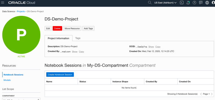
That’s the Project created.
2 – Create a Notebook
After creating a project (see above) you can not create one or many Notebook Sessions.
To create a Notebook Session click on the Create Notebook Session button (see the above image). This will create a VM to contain your notebook and associated work. Just like all VM in Oracle Cloud, they come in various different shapes. These can be adjusted at a later time to scale up and then back down based on the work you will be performing.
The following example creates a Notebook Session using the basic VM shape. I call the Notebook ‘DS-Demo-Notebook’. I also set the Block Storage size to 50G, which is the minimum value. The VNC details have been defaulted to those assigned to the Compartment. Click Create button at the bottom of the page.

The Notebook Session VM will be created. This might take a few minutes. When created you will see a screen like the following.
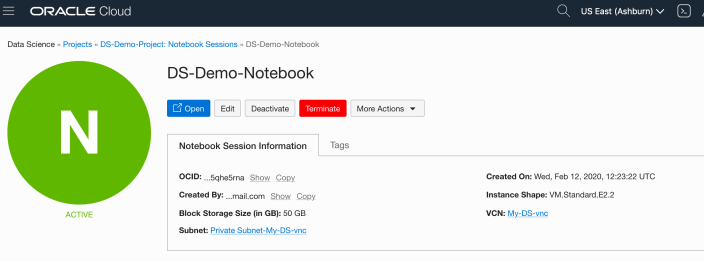
3 – Open the Notebook
After completing the above steps you can now open the Notebook Session in your browser. Either click on the Open button (see above image), or copy the link and share with your data science team.
Important: There are a few important considerations when using the Notebooks. While the session is running you will be paying for it, even if the session got terminated at the browser or you lost connect. To manage costs, you may need to stop the Notebook session. More details on this in a later post.
After clicking on the Open button, a new browser tab will open and will ask you to log-in.

After logging in you will see your Notebook.

4 – Explore the Notebook Environment
The Notebook comes pre-loaded with lots of goodies.
The menu on the left-hand side provides a directory with lots of sample Notebooks, access to the block storage and a sample getting started Notebook.

When you are ready to create your own Notebook you can click on the icon for that.

Or if you already have a Notebook, created elsewhere, you can load that into your OCI Data Science environment.

The uploaded Notebook will appear in the list on the left-hand side of the screen.
OCI Data Science – Initial Setup and Configuration
After a very, very, very long wait (18+ months) Oracle OCI Data Science platform is now available.
But before you jump straight into using OCI Data Science, there is a little bit of setup required for your Cloud Tenancy. There is the easy simple approach and then there is the slightly more involved approach. These are
- Simple approach. Assuming you are just going to use the root tenancy and compartment, you just need to setup a new policy to enable the use of the OCI Data Science services. This assuming you have your VNC configuration complete with NAT etc. This can be done by creating a policy with the following policy statement. After creating this you can proceed with creating your first notebook in OCI Data Science.
allow service datascience to use virtual-network-family in tenancy

- Slightly more complicated approach. When you get into having a team based approach you will need to create some additional Oracle Cloud components to manage them and what resources are allocated to them. This involved creating Compartments, allocating users, VNCs, Policies etc. The following instructions brings you through these steps
IMPORTANT: After creating a Compartment or some of the other things listed below, and they are not displayed in the expected drop-down lists etc, then either refresh your screen or log-out and log back in again!
1. Create a Group for your Data Science Team & Add Users
The first step involves creating a Group to ‘group’ the various users who will be using the OCI Data Science services.
Go to Governance and Administration ->Identity and click on Groups.
Enter some basic descriptive information. I called my Group, ‘my-data-scientists’.


Now click on your Group in the list of Groups and add the users to the group.
You may need to create the accounts for the various users.

2. Create a Compartment for your Data Science work
Now create a new Compartment to own the network resources and the Data Science resources.
Go to Governance and Administration ->Identity and click on Compartments.
Enter some basic descriptive information. I’ve called my compartment, ‘My-DS-Compartment’.


3. Create Network for your Data Science work
Creating and setting up the VNC can be a little bit of fun. You can do it the manual way whereby you setup and configure everything. Or you can use the wizard to do this. I;m going to show the wizard approach below.
But the first thing you need to do is to select the Compartment the VNC will belong to. Select this from the drop-down list on the left hand side of the Virtual Cloud Network page. If your compartment is not listed, then log-out and log-in!


To use the wizard approach click the Networking QuickStart button.
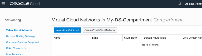
Select the option ‘VCN with Internet Connectivity and click Start Workflow, as you will want to connect to it and to allow the service to connect to other cloud services.

I called my VNC ‘My-DS-vnc’ and took the default settings. Then click the Next button.

The next screen shows a summary of what will be done. Click the Create button, and all of these networking components will be created.

All done with creating the VNC.
4. Create required Policies enable OCI Data Science for your Compartment
There are three policies needed to allocated the necessary resources to the various components we have just created. To create these go to Governance and Administration ->Identity and click on Policies.
Select your Compartment from the drop-down list. This should be ‘My-DS-Compartment’, then click on Create Policy.
The first policy allocates a group to a compartment for the Data Science services. I called this policy, ‘DS-Manage-Access’.
allow group My-data-scientists to manage data-science-family in compartment My-DS-Compartment
The next policy is to give the Data Science users access to the network resources. I called this policy, ‘DS-Manage-Network’.
allow group My-data-scientists to use virtual-network-family in compartment My-DS-Compartment
And the third policy is to give Data Science service access to the network resources. I called this policy, ‘DS-Network-Access’.
allow service datascience to use virtual-network-family in compartment My-DS-Compartment
Job Done 🙂
You are now setup to run the OCI Data Science service. Check out my Blog Post on creating your first OCI Data Science Notebook and exploring what is available in this Notebook.
Python-Connecting to multiple Oracle Autonomous DBs in one program
More and more people are using the FREE Oracle Autonomous Database for building new new applications, or are migrating to it.
I’ve previously written about connecting to an Oracle Database using Python. Check out that post for details of how to setup Oracle Client and the Oracle Python library cx_Oracle.
In thatblog post I gave examples of connecting to an Oracle Database using the HostName (or IP address), the Service Name or the SID.
But with the Autonomous Oracle Database things are a little bit different. With the Autonomous Oracle Database (ADW or ATP) you will need to use an Oracle Wallet file. This file contains some of the connection details, but you don’t have access to ServiceName/SID, HostName, etc. Instead you have the name of the Autonomous Database. The Wallet is used to create a secure connection to the Autonomous Database.
You can download the Wallet file from the Database console on Oracle Cloud.

Most people end up working with multiple database. Sometimes these can be combined into one TNSNAMES file. This can make things simple and easy. To use the download TNSNAME file you will need to set the TNS_ADMIN environment variable. This will allow Python and cx_Oracle library to automatically pick up this file and you can connect to the ATP/ADW Database.
But most people don’t work with just a single database or use a single TNSNAMES file. In most cases you need to switch between different database connections and hence need to use multiple TNSNAMES files.
The question is how can you switch between ATP/ADW Database using different TNSNAMES files while inside one Python program?
Use the os.environ setting in Python. This allows you to reassign the TNS_ADMIN environment variable to point to a new directory containing the TNSNAMES file. This is a temporary assignment and over rides the TNS_ADMIN environment variable.
For example,
import cx_Oracle
import os

os.environ['TNS_ADMIN'] = "/Users/brendan.tierney/Dropbox/wallet_ATP"

p_username = ''p_password = ''p_service = 'atp_high'
con = cx_Oracle.connect(p_username, p_password, p_service)

print(con)
print(con.version)
con.close()
I can now easily switch to another ATP/ADW Database, in the same Python program, by changing the value of os.environ and opening a new connection.
import cx_Oracle
import os

os.environ['TNS_ADMIN'] = "/Users/brendan.tierney/Dropbox/wallet_ATP"
p_username = ''
p_password = ''
p_service = 'atp_high'
con1 = cx_Oracle.connect(p_username, p_password, p_service)
...
con1.close()

...
os.environ['TNS_ADMIN'] = "/Users/brendan.tierney/Dropbox/wallet_ADW2"
p_username = ''
p_password = ''
p_service = 'ADW2_high'
con2 = cx_Oracle.connect(p_username, p_password, p_service)
...
con2.close()
As mentioned previously the setting and resetting of TNS_ADMIN using os.environ, is only temporary, and when your Python program exists or completes the original value for this environment variable will remain.
Applying a Machine Learning Model in OAC
There are a number of different tools and languages available for machine learning projects. One such tool is Oracle Analytics Cloud (OAC). Check out my article for Oracle Magazine that takes you through the steps of using OAC to create a Machine Learning workflow/dataflow.

Oracle Analytics Cloud provides a single unified solution for analyzing data and delivering analytics solutions to businesses. Additionally, it provides functionality for processing data, allowing for data transformations, data cleaning, and data integration. Oracle Analytics Cloud also enables you to build a machine learning workflow, from loading, cleaning, and transforming data and creating a machine learning model to evaluating the model and applying it to new data—without the need to write a line of code. My Oracle Magazine article takes you through the various tasks for using Oracle Analytics Cloud to build a machine learning workflow.
That article covers the various steps with creating a machine learning model. This post will bring you through the steps of using that model to score/label new data.
In the Data Flows screen (accessed via Data->Data Flows) click on Create. We are going to create a new Data Flow to process the scoring/labeling of new data.

Select Data Flow from the pop-up menu. The ‘Add Data Set’ window will open listing your available data sets. In my example, I’m going to use the same data set that I used in the Oracle Magazine article to build the model. Click on the data set and then click on the Add button.

The initial Data Flow will be created with the node for the Data Set. The screen will display all the attributes for the data set and from this you can select what attributes to include or remove. For example, if you want a subset of the attributes to be used as input to the machine learning model, you can select these attributes at this stage. These can be adjusted at a later stages, but the data flow will need to be re-run to pick up these changes.

Next step is to create the Apply Model node. To add this to the data flow click on the small plus symbol to the right of the Data Node. This will pop open a window from which you will need to select the Apply Model.

A pop-up window will appear listing the various machine learning models that exist in your OAC environment. Select the model you want to use and click the Ok button.


The next node to add to the data flow is to save the results/outputs from the Apply Model node. Click on the small plus icon to the right of the Apply Model node and select Save Results from the popup window.

We now have a completed data flow. But before you finish edit the Save Data node to give a name for the Save Data Set, and you can edit what attributes/features you want in the result set.

You can now save and run the Data Flow, and view the outputs from applying the machine learning model. The saved data set results can be viewed in the Data menu.

Oracle Magazine articles
Over the past few weeks I’ve had a couple of articles published with Oracle Magazine and these can be viewed on their website.
The first article is titled ‘Quickly Create Charts and Graphs of You Query Data‘ using Oracle Machine Learning Notebooks.

The second article is titled ‘REST-Enabling Oracle Machine Learning Models‘.

Click on the above links to check out those articles and check out the Oracle Magazine website for lots more articles and content.
There will be a few more Oracle Magazine articles coming out over the next few months.
Creating a VM on Oracle Always Free
I’m going to create a new Cloud VM to host some of my machine learning work. The first step is to create the VM before installing the machine learning software.
That’s what I’m going to do in this blog post and the next blog post. In this blog post I’ll step through how to setup the VM using the Oracle Always Free cloud offering. In the next I’ll go through the machine learning software install and setup.
Step 1 – Create a ssh key/file
Whatever your preferred platform for your day to day computer there will be software available for you to generate a ssh key file. You will need this when creating the VM and for when you want to login in to VM on the command line. My day-to-day workhorse is a Mac, and I used the following command to create the ssh key file.
ssh-keygen -t rsa -N "" -b 2048 -C "myOracleCloudkey" -f myOracleCloudkey
Step 2 – Login and Select create VM
Log into your Oracle Cloud Always Free account.

Select Create a VM Instance.

Step 3 – Configure the VM
Give the instance a name. I called mine ‘b01-vm-1‘

Expand the networks section by clicking on Show Shape, Network and Storage Options. Set the IP address to be public.

Scroll down to the ssh section. Select the ssh file you created earlier.

Click on the Create button.
That’s it, all done. Just wait for the VM to be created. This will takes a few seconds.

After the VM is created the IP address will be listed on this screen. Take note of it.
Step 4 – Connect and log into the VM
We can not log into the VM using ssh, to prove that it exists, using the command
ssh -i <name of ssh file> opc@<ip address of VM>
When I use this command I get the following:
ssh -i XXXXXXXXXX opc@XXX.XXX.XXX.XXX
The authenticity of host 'XXX.XXX.XXX.XXX (XXX.XXX.XXX.XXX)' can't be established.
ECDSA key fingerprint is SHA256:fX417Z1yFoQufm7SYfxNi/RnMH5BvpvlOb2gOgnlSCs.
Are you sure you want to continue connecting (yes/no)? yes
Warning: Permanently added 'XXX.XXX.XXX.XXX' (ECDSA) to the list of known hosts.
Enter passphrase for key 'XXXXXXXXXX':
[opc@b1-vm-01 ~]$ pwd
/home/opc

[opc@b1-vm-01 ~]$ df
Filesystem   1K-blocks     Used Available Use%  Mounted on
devtmpfs        469092        0    469092   0%  /dev
tmpfs           497256        0    497256   0%  /dev/shm
tmpfs           497256     6784    490472   2%  /run
tmpfs           497256        0    497256   0%  /sys/fs/cgroup
/dev/sda3     40223552  1959816  38263736   5%  /
/dev/sda1       204580     9864    194716   5%  /boot/efi
tmpfs            99452        0     99452   0%  /run/user/1000
And there we have it. A VM setup on Oracle Always Free.
Next step is to install some Machine Learning software.
Changing PDB/CDB spfile parameters
When working with a Oracle database hosted on the Oracle cloud (not an Autonomous DB), I recently had the need to change/increase the number of processes for the database. After a bit of researching it looked liked I just had to make the change to the SPFILE and that would be it.
I needed to change/increase the PROCESSES parameter for the CDB and the PDB. Following the multitude of advice on the internet, I ssh into the DB server, found the SPFILE and changed it.
I bounced the DB and when I connected to the PDB, I found the number for PROCESSES was still the same as the old/original value. Nothing had changed.
By default the initialization parameter for the PDB inherit the values from the parameters for the CDB. But this didn’t seem to be the case.
After a bit more research, I needed to set this parameter for the CDB and the PDB. But no luck finding a parameter file for the PDB. It turns out the parameters for the PDB are set at the metadata level, and I needed to change the parameter there.
What I had to do was to change the value when connected to it using SQL*Plus, SQL Dev etc. So, How did I change the parameter value.
Using SQL Developer as my tool, I connected as SYSDBA to my PDB. Then ran,
alter session set container = cdb$root
Now change the parameter value.
alter system set processes = 1200 scope=both
I then bounced the database, logged back into my PDB as system and checked the parameter values. It worked. This was such a simple solution and it worked for me, but there was way too many articles, blog posts, etc out there that didn’t work. Something I’ll need to investigate later is, did I need to connect to the CDB? could I have just run the second command only? I need to setup a different/test DB and see.
OML Workspace Permissions
When working with Oracle Machine Learning (OML) you are creating notebooks which focus on a particular data exploration and possibly some machine learning. Despite it’s name, OML is used extensively for data discovery and data exploration.
One of the aims of using OML, or notebooks in general, is that these can be easily shared with other people either within the same team or beyond. Something to consider when sharing notebooks is what you are allowing other people do with your notebook. Without any permissions you are allowing people to inspect, run and modify the notebooks. This can be a problem because those people you are sharing with may or may not be allowed to make modification. Some people should be able to just view the notebook, and others should be able to more advanced tasks.
With OML Notebooks there are four primary types of people who can access Notebooks and these can have different privileges. These are defined as
- Developer : Can create new notebooks withing a project and workspace but cannot create a workspace or a project. Can create and run a notebook as a scheduled job.
- Viewer : They can just view projects, Workspaces and notebooks. They are not allowed to create or run anything.
- Manager : can create new notebooks and projects. But only view Workspaces. Additionally they can schedule notebook jobs.
- Administrators : Administrators of the OML environment do not have any edit capabilities on notebooks. But they can view them.

OML Notebooks Interpreter Bindings
When using Oracle Machine Learning notebooks, you can export and import these between different projects and different environments (from ADW to ATP).
But something to watch out for when you import a notebook into your ADW or ATP environment is to reset the Interpreter Bindings.
When you create a new OML Notebook and build it up, the various Interpreter Bindings are automatically set or turned on. But for Imported OML Notebooks they are not turned on.
I’m assuming this will be fixed at some future point.
If you import an OML Notebook and turn on the Interpreter Bindings you may find the code in your notebook cells running very slowly
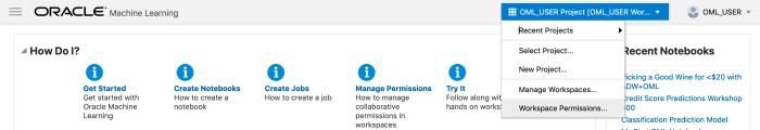
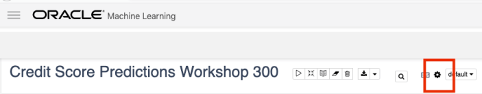
To turn on these binding, click on the options icon as indicated by the red box in the following image.
You will get something like the following being displayed. None of the bindings are highlighted.
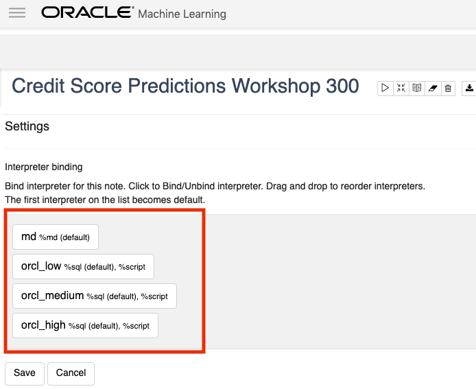
To enable the Interpreter Bindings just click on each of these boxes. When you do this each one will be highlighted and will turn a blue color.
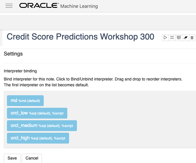
All done! You can now run your OML Notebooks without any problems or delays.
ADW – Loading data using Object Storage
There are a number of different ways to load data into your Autonomous Data Warehouse (ADW) environment. I’ll have posts about these alternatives.
In this blog post I’ll go through the steps needed to load data using Object Storage. This might appear to have a large-ish number of steps, but once you have gone through it and have some of the parts already setup and configuration from your first time, then the second and subsequent times will be easier.
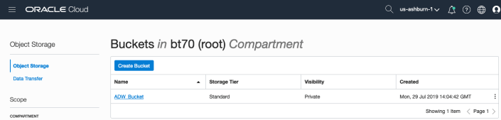
After logging into your Oracle Cloud dashboard, select Object Storage from the side menu.

Then click on the Create Bucket button.

Enter a name for the Object Storage bucket, take the defaults for the for the rest, and click on the Create Bucket button at the bottom. In my example, I’ve called the bucket ‘ADW_Bucket’.

Click on the name of the bucket in the list.
And then click Upload Objects button.

In the Upload Objects window, browse for the file(s) you want to upload.


Then click on the Upload Objects button on the Upload Objects window. After a few moments you will see a message saying the file(s) have been uploaded. Click on the Close window.
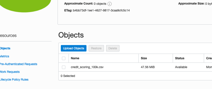
Click into the Object details and take a note/copy of the URL Path. You will need this later
To load data from the Oracle Cloud Infrastructure(OCI) Object Storage you will need an OCI user with the appropriate privileges to read data (or upload) data to the Object Store. The communication between the database and the object store relies on the Swift protocol and the OCI user Auth Token. Go back to the menu in the upper left and select users.


Then click on the user name to view the details. This is probably your OCI username.
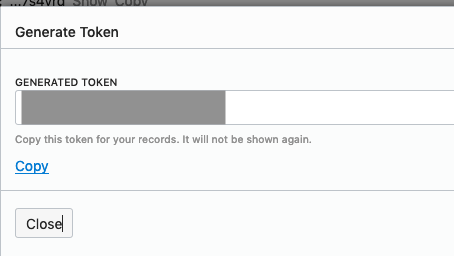
On the left hand side of the page click Auth Tokens, and then click on Generate Token button. Give a name for the token e.g ADW_TOKEN, and then generate token.
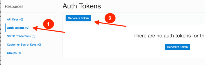
Save the generated token to use later.
Open SQL Developer and setup a connection to your OML User/schema. When connected the next steps is to authenticate with the Object storage using your OCI username and the Auth Token, generated above.
BEGIN
  DBMS_CLOUD.CREATE_CREDENTIAL(
    credential_name => 'ADW_TOKEN',
    username => '<your cloud username>',
    password => '<generated auth token>'
  );
END;
If successful you should get the following message. If not then you probably entered something incorrectly. Go back and review the previous steps
PL/SQL procedure successfully completed.
Next, create a table to store the data you want to import. For my table the create table is the following. [It is one of the sample data sets for OML, and I’ve made the create table statement compact to save space in this post]
create table credit_scoring_100k
( customer_id number(38,0), age number(4,0), income number(38,0), marital_status varchar2(26 byte),
number_of_liables number(3,0), wealth varchar2(4000 byte), education_level varchar2(26 byte),
tenure number(4,0), loan_type varchar2(26 byte), loan_amount number(38,0),
loan_length number(5,0), gender varchar2(26 byte), region varchar2(26 byte),
current_address_duration number(5,0), residental_status varchar2(26 byte),
number_of_prior_loans number(3,0), number_of_current_accounts number(3,0),
number_of_saving_accounts number(3,0), occupation varchar2(26 byte),
has_checking_account varchar2(26 byte), credit_history varchar2(26 byte),
present_employment_since varchar2(26 byte), fixed_income_rate number(4,1),
debtor_guarantors varchar2(26 byte), has_own_phone_no varchar2(26 byte),
has_same_phone_no_since number(4,0), is_foreign_worker varchar2(26 byte),
number_of_open_accounts number(3,0), number_of_closed_accounts number(3,0),
number_of_inactive_accounts number(3,0), number_of_inquiries number(3,0),
highest_credit_card_limit number(7,0), credit_card_utilization_rate number(4,1),
delinquency_status varchar2(26 byte), new_bankruptcy varchar2(26 byte),
number_of_collections number(3,0), max_cc_spent_amount number(7,0),
max_cc_spent_amount_prev number(7,0), has_collateral varchar2(26 byte),
family_size number(3,0), city_size varchar2(26 byte), fathers_job varchar2(26 byte),
mothers_job varchar2(26 byte), most_spending_type varchar2(26 byte),
second_most_spending_type varchar2(26 byte), third_most_spending_type varchar2(26 byte),
school_friends_percentage number(3,1), job_friends_percentage number(3,1),
number_of_protestor_likes number(4,0), no_of_protestor_comments number(3,0),
no_of_linkedin_contacts number(5,0), average_job_changing_period number(4,0),
no_of_debtors_on_fb number(3,0), no_of_recruiters_on_linkedin number(4,0),
no_of_total_endorsements number(4,0), no_of_followers_on_twitter number(5,0),
mode_job_of_contacts varchar2(26 byte), average_no_of_retweets number(4,0),
facebook_influence_score number(3,1), percentage_phd_on_linkedin number(4,0),
percentage_masters number(4,0), percentage_ug number(4,0),
percentage_high_school number(4,0), percentage_other number(4,0),
is_posted_sth_within_a_month varchar2(26 byte), most_popular_post_category varchar2(26 byte),
interest_rate number(4,1), earnings number(4,1), unemployment_index number(5,1),
production_index number(6,1), housing_index number(7,2), consumer_confidence_index number(4,2),
inflation_rate number(5,2), customer_value_segment varchar2(26 byte),
customer_dmg_segment varchar2(26 byte), customer_lifetime_value number(8,0),
churn_rate_of_cc1 number(4,1), churn_rate_of_cc2 number(4,1),
churn_rate_of_ccn number(5,2), churn_rate_of_account_no1 number(4,1),
churn_rate__of_account_no2 number(4,1), churn_rate_of_account_non number(4,2),
health_score number(3,0), customer_depth number(3,0),
lifecycle_stage number(38,0), credit_score_bin varchar2(100 byte));
After creating the table, you are ready to import the data from Object storage. To do this you will need to use the DBMS_COULD PL/SQL package.
begin
   dbms_cloud.copy_data(
   table_name =>'credit_scoring_100k',
   credential_name =>'ADW_TOKEN',
   file_uri_list => '<url of file in your Object Store bucket, see comment earlier in post>',
   format => json_object('ignoremissingcolumns' value 'true', 'removequotes' value 'true', 'dateformat' value 'YYYY-MM-DD HH24:MI:SS', 'blankasnull' value 'true', 'delimiter' value ',', 'skipheaders' value '1')
);
end;
All done.
You can now query the data and use with Oracle Machine Learning, etc.
[I said at the top of the post there are other methods available. More on this in other posts]

You must be logged in to post a comment.