
Machine Learning
OML4Py – AutoML – Oracle GUI for AutoML
In addition to the new AutoML features with OML4Py (Oracle Machine Learning for Python), which is currently available on ADW/ATP using Oracle Machine Learning (OML) Notebooks, Oracle has just released a GUI for AutoML.
As with all new releases there are a few things that Oracle need to tidy up with the interface and CX with this GUI. I’m sure these will be corrected/updated quietly behind the scenes and we will gradually see these improvements over the weeks to come (after product release). Part of the joys of cloud first deployment.
The initial release of AutoML GUI is SO SLOW. It is several, several times slower than trying to do the same task in OML4Py. Plus the Algorithms used and models created seem to be different. Maybe this is down to the “meta-learning” AutoML uses, but for repeatability and ensuring confidence with of outputs, some additional work is needed otherwise it is unreliable and people won’t use something that is unreliable.
To illustrate how to use the AutoML GUI, I’m going to use the same example and same Oracle Cloud environment I’ve used to illustrate the other ways of running AutoML using OML4Py (see post 1, see post 2).
The AutoML GUI can be accessed from the main OML Notebooks welcome page. On the next webpage, called AutoML Experiment, click on the Create button.

The Create Experiment page allows you to specify the required details for you AutoML experiment. Although this tool is aims at non-technical people, they still require a certain degree of knowledge of Machine Learning and what the different terms mean! On the Create Experiment page enter the following details, and enter them in this order. Numbers below correspond to numbers on image below
- Name of experiment – free format text – enter a meaningful name
- Data Source – Click on Magnifying Glass – Select your Schema, and Table/View from the list
- Predict – what attribute is the Target variable/column
- Case ID – Select attribute that is unique e.g. PK, or some other attribute. Selecting an attribute for this is not necessary
- Features – Exclude any attributes you don’t want included, for example attributes that are correlated to the target values
You can now run the AutoML process by clicking the Start button at the top of the page (6).

But maybe before you do this, you can look at the Additional Settings, and alter these if you want or just leave them as they are

After clicking the Start button, you are given two options or modes. You can run the AutoML Experiment with “Faster Results” or with “Better Accuracy”. Both of these are SLOW to execute, but I’d advice running using Both options/modes to see how the results differ. This does require you to setup two version of the same AutoML Experiment!
When the AutoML Experiment is running, see image below, the dashboard displays results are each part of the experiment completes. These include the Algorithms, the accuracy levels and the Features/Attributes that are important.

The AutoML Experiment will eventually finish! Even after displaying the details of the last algorithm in the Leaders Board, it will keep running for some time before completing. Initially the dashboard will just display Accuracy for the model. You can expand this list of evaluation metrics by clicking the ‘Metrics’ located just under the Leader Board title, and selecting the additional evaluation metrics from the list. These will now be displayed on the Leaders Board.

That’s it! Relatively simple to use, but you do still know what you are doing, and it isn’t really aimed at novices despite some of the marketing.
One final feature that is kind of nice is the ‘Create Notebook’. Located in Leader Board section, select one of the models, and then click on ‘Create Notebook’ and it will create an OML Notebook for you based on the model you have selected. You will be promoted to give the notebook a name. A message will be displayed at the top of the webpage saying ‘…notebook successfully created’. Go to your list of Notebooks and open it. It will be a basic notebook with code to create/define the data set, setup model settings, create the model, display model details and use the model to label a data set.

AutoML is just too slow at the moment (I’ve tested with several data sets of different sizes). Start the process and go for lunch. It might be finished when you get back! I’ve been told things would run a lot quicker if I wasn’t using the Free Tier. I hope that is true, but how many people have easy access to such an environment to test this? Not many, including myself, which makes it difficult to test and compare the results. The Free Tier is the gateway for people get to try new Oracle products. First impression are important.
I mentioned earlier I used the same data set and Oracle Cloud environment when I showed how to use AutoML in OML4Py (using OML Notebooks). The results from OML4Py AutoML are different to those show above using AutoML (G)UI. Getting different results with similar setttings/configurations is very confusing. Which approach should be used for AutoML? Can you trust the results from AutoML if you are getting different results? If the data scientist uses OML4Py and the data analyst uses the AutoML GUI, then there should be some commonality in what is produced by these same/similar AutoML. Realiability and reproducibility is vital in Data Science, Machine Learning, etc.
In my tests, there was no similarity/commonality with the outputs from AutoML, that was my experience. In such a situation where different AutoML outputs are produced which one should we believe/trust? Who will the business users believe? Who is doing it correctly? Who is producing results the business can rely upon?
OML4Py – AutoML – An Example
OML4Py (Oracle Machine Learning for Python) is Oracle’s offering where you can use Python commands to process and analyse data in an Oracle Database without having to write any SQL. OML4Py, via it’s transparency layer, translates Python code into SQL, executes it in the Database and then presents the results back to you in your Python environment. The examples shown in this post used the OML Notebooks available with Autonomous Databases on Oracle Cloud.
[Warning: the functionality available with initial release of OML4Py is very limited and may not suit most Python developers. Hopefully this will be addressed in later releases]
One of the features of OML4Py is Automated Machine Leaning (AutoML). At some point in the near future Oracle will have a GUI interface for AutoML, which will save you from having to write any code, such as the example in this post. See my previous blog post about AutoML. It is a general discussion on AutoML and some things you need to be careful with. Also, be careful of the marketing around AutoML from all vendors. The reality doesn’t necessarily live up to marketing

OML4Py has a couple of approaches you can follow to Automatically generate a Machine Learning Model (see previous blog post). The first of these can be considered the Black Box approach for AutoML, and the example below illustrates an example of this. The more detailed version of AutoML will be covered in a later post.
[Info: I’m using Oracle Free Tier Database. At time of writing this post OML4Py is only available with Oracle Autonomous 19c]
But before look at these, the first step we need to do is setup the data set to use for AutoML. I’ll be using the popular Portuguese Bank data set. Each code snippets shown below are for a one cell in my OML Notebooks. The data set exists as a table in my schema called BANK_ADDITIONAL_FULL. The sync command creates a proxy object in the notebook session pointing to the table in the DB. No data is copied into the notebook.
%python
import oml
from oml import automl
import pandas as pd
%python
oml_bank = oml.sync(table = 'BANK_ADDITIONAL_FULL')
type(oml_bank)
Let’s explore the data. Remember the data lives in a table in the DB and only the results are displayed
%python
oml_bank.head()

%python
oml_bank.describe()

Now remove one attribute from data set and at the sample time setup the dataframes for input to the ML. This is highly correlated to the the target variable.
%python
oml_bank_X, oml_bank_y = oml_bank.drop('TARGET_Y'), oml_bank['TARGET_Y']
Finally, we can now look at the first of the AutoML options, the black box option. This uses the AutoML ModelSelection function. Using this you can define the type of machine learning to perform (‘classification) and set some additional parameters. The parallel parameter will probably not have too much of an effect when using the Oracle Free Tier, but will certainly improved performance when using additional compute resources.
The example below is very simple and the setup of it is very simple. The ModelSelection function sets up the parameters for the AutoML to function. The ‘select’ function runs the AutoML based on those parameters along with some additional ones. These parameters and the additional ones available are explained below, after this first example.
%python
ms_bank = automl.ModelSelection(mining_function='classification', parallel=4)
ModelSelection can have the following parameters. The possible values for each are listed with the value in bold being the default value:
- mining_function : the type of ML to preform, only two option available for this, classification or regression
- score_metric: what metric to use for evaluating the models. Defaults for binary and multi classification balanced_accuracy is used and default for regression is neg_mean_squared_error. Other options for regression include r2, neg_mean_absolute_error and neg_median_absolute_error. For classification other options include, accuracy, f1, precision, recall, roc_auc, f1_micro, f1_macro, f1_weighted, recall_micro, recall_macro, recall_weighted, precision_micro, precision_macro, precision_weighted
- parallel: degree of parallelism to use, None or a number.
Having defined ModelSelection settings, we can move onto using it to preform (black box) AutoML, using the ‘select’ function. Oracle doesn’t tell us what it does inside this black box except that it uses ML and meta-learning techniques to work out which algorithms to use, what subsets of the original data set to use to give use a optimal outcome. It’s there secret recipe!
The ‘select’ function elevates all the available algorithms, creating models for each or a subset of them based on the meta-learning, and returns the “best” one. The function returns just one model, which is the “best”. The value set for ‘k’ tells the function how many of the “best” or top models created, how many of these to tune before returning the “best” one.
Now, let’s run an example of the ‘select’ function and what parameters is can have
- X: input data set consisting of the columns to use for Training.
- y: the column containing the Target variable.
- case_id: columns name of case_id, default is None. If supplied can be used for data sampling
- k: the number of (best) models to tune. Default is 3, but can be set to any number between one and eight, as setting it higher than that has no effect as there aren’t any more than that number of algorithms in the database!
- solver: allowed values are fast (default) and exhaustive. fast uses internal ML and meta-learning thereby reducing the search space. exhaustive will be slower as it will evaluate all algorithms and options for creating a model.
- cv: cross validation. Default is auto, but can be set to a number or set to None uses inputs defined in X_valid and y_valid defined below. auto will determine the number based on size of input data set, and when a number is provided will perform that number cross validation.
- adaptive_sampling: use adaptive sampling to reduce data set size to speed up runtime of ‘select’ function. Default is True, otherwise use False.
- X_valid: validation data set, default is None.
- y_valid: validation target column, default is None.
- time_budget: defines a time constraint on how how long, in seconds, to spend working out the solution. Default is None, or number for number of seconds. Useful for large data sets or for when you need a quicker results, and can be increased based on experimentation.
Here is a basic example of using the ‘select’ function, using the data frames created above as input, ‘k’ is set to five telling the function to tune the top five models created based on doing five fold cross-validation ‘cv’.
best_model = ms_bank.select(oml_bank_X, oml_bank_y, k=5, cv=5)
best_model
This returns the following model information. We are told the algorithm used (RandomForest), the tuned algorithm settings, and what attributes from the input data frame are used in the tuned model.
(
Algorithm Name: Random Forest

Mining Function: CLASSIFICATION

Target: TARGET_Y

Settings:
setting name setting value
0 ALGO_NAME ALGO_RANDOM_FOREST
1 CLAS_MAX_SUP_BINS 32
2 CLAS_WEIGHTS_BALANCED OFF
3 ODMS_DETAILS ODMS_DISABLE
4 ODMS_MISSING_VALUE_TREATMENT ODMS_MISSING_VALUE_AUTO
5 ODMS_RANDOM_SEED 0
6 ODMS_SAMPLING ODMS_SAMPLING_DISABLE
7 PREP_AUTO ON
8 RFOR_MTRY 10
9 RFOR_NUM_TREES 20
10 RFOR_SAMPLING_RATIO 0.5
11 TREE_IMPURITY_METRIC TREE_IMPURITY_ENTROPY
12 TREE_TERM_MAX_DEPTH 16
13 TREE_TERM_MINPCT_NODE 0.05
14 TREE_TERM_MINPCT_SPLIT 0.1
15 TREE_TERM_MINREC_NODE 10
16 TREE_TERM_MINREC_SPLIT 20

Attributes:
AGE
CAMPAIGN
CONS_CONF_IDX
CONS_PRICE_IDX
CONTACT
DEFAULT_VALUE
DURATION
EDUCATION
EMP_VAR_RATE
EURIBOR3M
JOB
MARITAL
MONTH
NR_EMPLOYED
PDAYS
POUTCOME
PREVIOUS

Partition: NO

, 'rf')
[I’ve found the Oracle Documentation for (initial release of) OML4Py lacking with information. Hopefully the documentation will be updated]
I’ve mentioned before you need to exercise some caution with using AutoML due to various potential legal and moral issues. Can they be used as a quick way get an idea if ML will produce useful insights for your data. But the results from it should never be used for making business decisions and never deployed in production. Use it as a starting point, from which to build out an ML solutions with humans making the decisions on what to use and why to use them.
For a more detailed, step-by-step approach to AutoML check out this next post for more.
[Warning: Based on the functionality currently available in this early release of OML4Py, you will be limited in what you can do, not just with AutoML but with other features of OML4Py. Maybe check back at a later time when it has matured and has way more functionality, allowing you to do something useful with it!]
AutoML, what is it good for? It Depends!
Automated Machine Learning (AutoML) seems to be everywhere and every Analytics product and SaaS offering seems to have some element of AutoML built into them. Part of the reason for this is because most of the market analysts, such as Gartner etc., have been rating Machine Learning (ML) products and services based on them having an AutoML feature.
Some of the benefits of AutoML is it will automatically generate a ML model for you without you having to worry about any of the technical details and the various statistical tests to measure if the model is useful. This kind of message has resulted is lots and lots of articles talking about the death of the Data Scientist, as they are no longer needed. We must remember ML is only one of the tools and skills of the data scientist.
This can all sound great. No need to hire these expensive data scientists, I can just use this AutoML software to create a ML model, for my data, and life will be good with all these wonderful predictions. Just think of the money I’ll be making and saving!
Where the fun comes into all of this is when someone issues legal proceedings based on what one of these AutoML models has predicted. The AutoML has made an incorrect prediction. The problem you now face, probably in court, is trying to justify the prediction by saying the machine/computer/algorithm made it, and you have no idea how or what it is doing to make the prediction. Good luck in a court explaining that to a judge and/or jury. Be prepared to hand over lots of money
What is missing is the human in the loop, and in most cases this will be the data scientist or machine learning engineer (or someone else with a really cool job title). Part of their job is to evaluate lots of difference models for you data (remember they will create lots and lots of models and not just one!), determine (from experimentation) what algorithms work best with your data and problem, optimize these models and assess the impact of changing hyperparameters, look at how these ML models are behaving, are there any biases in the model or data, use a wide variety of statistic tests to assess the models, examine how the model works with different sub-parts of the data (customers), look at any potential legal and legislative issues not just in one geographic but across many disparate regions all of which have different legal requirements, etc.
As you can see there are many additional tasks beyond the ML steps needed to create, verify and select a ML to use. All of this is before you look at how it can be deployed in your production systems/architecture and building out you MLOps.
One importing characteristic of having the human in the loop is Explainability. Explainability of the process followed, what models were produced, the effect of tuning and opimizing, possible biases and mitigating steps, etc etc The list goes on and on. This the role of the data scientist and now it might look like a good idea to hire a good data scientist who understands all of this.

Taking a little step back, AutoML is kind of good cool feature/tool. A lot of the main steps of creating all those ML models, tuning them and evaluating them, etc can be very boring work. You do same steps for each model and do it all over again for the next, and so on for the tens or hundreds of models you will be creating. Most data scientists will have scripts in their toolbox (based from their experience) to automatically perform all of these steps and output the results. I mentioned the word experience in the last sentence. It can take a bit of time to build up to this. The AutoML products will do all of this automatically for you hence you don’t have to hire a data scientist to do it (see what I said above about this).
I mentioned above some of the challenges and the need to keep a human in the loop. AutoML can be seen as another tool to assist the data scientist and not to replace them. AutoML can be used to to help the data scientist work towards identifying what ML models to use. But this can be a bit of a challenge to do. It depends on what product or library you use. Some AutoML solutions act as a black box. Kind of like the image at the top of this post. These are simple to use but the draw back is there is not explainability or ability of the data scientist to really assess what is happening at each step. There are AutoML products/solutions that allow you to inspect and monitor what is happening at each step within AutoML. The diagram given able is one example of this. This allows for the human in the loop and allows for explainability. If the data scientist sees some unusual direction being taken by AutoML they can see where and why this is happening and can take corrective action. AutoML isn’t a black box in this scenario.
I mentioned above, AutoML can be another tool for the data scientist to use. Look on AutoML as quick way to see what might be possible. Using the information from each step of AutoML, the data scientist can use this information to guide them towards creating a more suitable and usable ML model, and do so in perhaps a slightly shorter space of time.
Going back to the title of the post ‘AutoML, what is it good for?’, the answer really is ‘It Depends!’, but if you do use it, be careful how you use the models and results beyond doing some simple investigation. And be careful of product offerings saying you don’t need anything else.
Collection of Oracle 21c posts on new Machine Learning and Statistical functions
Oracle 21c was officially released a few days about and this post contains links to some blog posts I’ve written on new machine learning and statistical functions in the new Oracle 21c.
- Adam Optimization Solver for Neural Network Algorithm
- MSET-SPRT Algorithm
- XGBoost Algorithm
- Measuring SKEWNESS Function
- Measuring tailedness of data with KURTOSIS Function
I also have posts on new OML4Py and AutoML too, and I’ll have a different set of posts for those, so look out them.
Also check out my previous blog post that covers new machine learning feature introduced in Oracle 19c.
2020 Books on Data Science and Machine Learning
2020 has been an interesting year. Not for the obvious topic, but for new books on Data Science and Machine Learning. The list below are some of my favorite books from 2020. Making the selection was difficult. Some months had a large number of releases and some were a bit quieter. The books below are listed based on their release date and are not ranked in any way. I’ve included links to these books on Amazon (.com, .uk and .de).
 |
 |
 |
|
| January
Everyone wants to work in Data Science, but where and how do you start. Aimed at beginners with guidance without the technical. High level, not for everyone. |
February
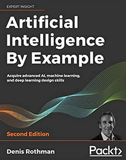
Taking ML to the next stage creating AI application. How to do it with examples across a number of areas. |
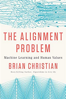
March
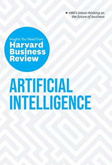
A guide for those wary of impact of technology’s and for those who are enthusiastic about where AI is taking us. |
|
 |
 |
 |
|
| April
AI Ethics was one of the topic topics for 2020. Covers the philosophical aspects along with the technical one.s |
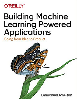
May
Covering the life-cyle of building ML application, showing all that it entails and how ML plays a small part in the overall solution |
June
From covering the basics of NLP, it builds on this to include in application, how to use in different industries and within project teams. |
|
 |
 |
 |
|
| July
With by Thomas Davenport and others, and is a good addition to his other books. Consisting of interviews, research and analysis on how to win with ML & AI. |
August
I was invited to contribute a couple of chapters to this book, along with well known names in areas of DS, ML & AI |
September
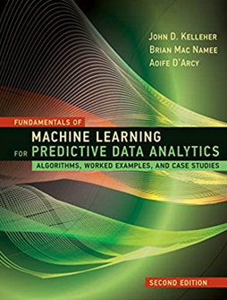
Building upon the success of their 1st edition, the 2nd edition comes with more example and extra chapters. |
|
 |
 |
 |
|
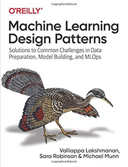
| October
ML & AI is not perfect. Lots can go wrong. Not just with the project but also with the implementation of the applications. Lots to thing about and consider. |
November
No one really builds ML algorithms. We build ML solutions and applications. But whats the best way to do this, from technical, organizational and ethical aspects. |
December
It was difficult to pick a book for this month. Lots of new releases and I haven’t received all my orders, at time of this post. Here is a book from July, and is related to an Automated Trading App I’ve been working on (and earning) for a couple of years. |
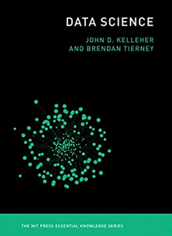
And to finish off the list I’m including this additional book. It wasn’t released this year. It was released in April 2018. It was a best seller on Amazon in 2018 and 2019! This was really exciting for us and we still amazed at how it it is still selling in 2020. It is currently, as of December 2020, listed in 8th place on the MIT Press Best Sellers list. It won’t be making any best seller list in 2020, but is still proving popular with many readers. To all of you who have bought this book, I’d like to say Thank You and wishing you all the best with 2021 and beyond.
Adding Text Processing to Classification Machine Learning in Oracle Machine Learning
One of the typical machine learning functions is Classification. This is in widespread use across most domains and geographic regions. I’ve written several blog posts on this topic over many years (and going back many, many year) on how to do this using Oracle Machine Learning (OML) (formally known as Oracle Advanced Analytic and in the Oracle Data Miner tool in SQL Developer). Just do a quick search of my blog to find some of these posts.
When it comes to Classification problems, typically the data set will be contain your typical categorical and numerical variables/features. The Automatic Data Preparation (ADP) feature of OML where it automatically pre-processes and transforms these variable for input to the machine learning algorithm. This greatly reduces the boring work of the data scientist and increases their productivity.
But sometimes data sets come with text descriptions. These will contain production descriptions, free format text, and other descriptive data, for example product reviews. But how can this information be included as part of the input data set to the machine learning algorithms. Oracle allows this kind of input data, and a letting bit of setup is needed to tell Oracle how to process the data set. This uses the in-database feature of Oracle Text.
The following example walks through an example of the steps needed to pre-process and include the text processing as part of the machine learning algorithm.
The data set: The data used to illustrate this and to show the steps needed, is a data set from Kaggle webiste. This data set contains 130K Wine Reviews. This data set contain descriptive information of the wine with attributes about each wine including country, region, number of points, price, etc as well as a text description contain a review of the wine.
The following are 2 files containing the DDL (to create the table) and then Import the data set (using sql script with insert statements). These can be run in your schema (in order listed below).
I’ll leave the Data Exploration to you to do and to discover some early insights.
The ML Question
I want to be able to predict if a wine is a good quality wine, based on the prices and different characteristics of the wine?
Data Preparation
To be able to answer this question the first thing needed is to define a target variable to identify good and bad wines. To do this create a new attribute/feature called POINTS_BIN and populate it based on the number of points a wine has. If it has >90 points it is a good wine, if <90 points it is a bad wine.
ALTER TABLE WineReviews130K_bin ADD POINTS_BIN VARCHAR2(15);

UPDATE WineReviews130K_bin
SET POINTS_BIN = 'GT_90_Points'
WHERE winereviews130k_bin.POINTS >= 90;

UPDATE WineReviews130K_bin
SET POINTS_BIN = 'LT_90_Points'
WHERE winereviews130k_bin.POINTS < 90;

alter table WineReviews130K_bin DROP COLUMN POINTS;
The DESCRIPTION column data type needs to be changed to CLOB. This is to allow the Text Mining feature to work correctly.
-- add a new column of data type CLOB
ALTER TABLE WineReviews130K_bin ADD (DESCRIPTION_NEW CLOB);

-- update new column with data from the DESCRIPTION attribute
UPDATE WineReviews130K_bin SET DESCRIPTION_NEW = DESCRIPTION;

-- drop the DESCRIPTION attribute from table
ALTER TABLE WineReviews130K_bin DROP COLUMN DESCRIPTION;

-- rename the new attribute to replace DESCRIPTION
ALTER TABLE WineReviews130K_bin RENAME COLUMN DESCRIPTION_NEW TO DESCRIPTION;
Text Mining Configuration
There are a number of things we need to define for the Text Mining to work, these include a Lexer, Stop Word list and preferences.
First define the Lexer to use. In this case we will use a basic one and basic settings
BEGIN
   ctx_ddl.create_preference('mylex', 'BASIC_LEXER');
   ctx_ddl.set_attribute('mylex', 'printjoins', '_-');
   ctx_ddl.set_attribute ( 'mylex', 'index_themes', 'NO');
   ctx_ddl.set_attribute ( 'mylex', 'index_text', 'YES');
END;
Next we can define a Stop Word List. Oracle Text comes with a predefined set of Stop Word lists for most of the common languages. You can add to one of those list or create your own. Depending on the domain you are working in it might be easier to create your own and it is very straight forward to do. For example:
DECLARE
   v_stoplist_name varchar2(100);
BEGIN
   v_stoplist_name := 'mystop';
   ctx_ddl.create_stoplist(v_stoplist_name, 'BASIC_STOPLIST');
   ctx_ddl.add_stopword(v_stoplist_name, 'nonetheless');
   ctx_ddl.add_stopword(v_stoplist_name, 'Mr');
   ctx_ddl.add_stopword(v_stoplist_name, 'Mrs');
   ctx_ddl.add_stopword(v_stoplist_name, 'Ms');
   ctx_ddl.add_stopword(v_stoplist_name, 'a');
   ctx_ddl.add_stopword(v_stoplist_name, 'all');
   ctx_ddl.add_stopword(v_stoplist_name, 'almost');
   ctx_ddl.add_stopword(v_stoplist_name, 'also');
   ctx_ddl.add_stopword(v_stoplist_name, 'although');
   ctx_ddl.add_stopword(v_stoplist_name, 'an');
   ctx_ddl.add_stopword(v_stoplist_name, 'and');
   ctx_ddl.add_stopword(v_stoplist_name, 'any');
   ctx_ddl.add_stopword(v_stoplist_name, 'are');
   ctx_ddl.add_stopword(v_stoplist_name, 'as');
   ctx_ddl.add_stopword(v_stoplist_name, 'at');
   ctx_ddl.add_stopword(v_stoplist_name, 'be');
   ctx_ddl.add_stopword(v_stoplist_name, 'because');
   ctx_ddl.add_stopword(v_stoplist_name, 'been');
   ctx_ddl.add_stopword(v_stoplist_name, 'both');
   ctx_ddl.add_stopword(v_stoplist_name, 'but');
   ctx_ddl.add_stopword(v_stoplist_name, 'by');
   ctx_ddl.add_stopword(v_stoplist_name, 'can');
   ctx_ddl.add_stopword(v_stoplist_name, 'could');
   ctx_ddl.add_stopword(v_stoplist_name, 'd');
   ctx_ddl.add_stopword(v_stoplist_name, 'did');
   ctx_ddl.add_stopword(v_stoplist_name, 'do');
   ctx_ddl.add_stopword(v_stoplist_name, 'does');
   ctx_ddl.add_stopword(v_stoplist_name, 'either');
   ctx_ddl.add_stopword(v_stoplist_name, 'for');
   ctx_ddl.add_stopword(v_stoplist_name, 'from');
   ctx_ddl.add_stopword(v_stoplist_name, 'had');
   ctx_ddl.add_stopword(v_stoplist_name, 'has');
   ctx_ddl.add_stopword(v_stoplist_name, 'have');
   ctx_ddl.add_stopword(v_stoplist_name, 'having');
   ctx_ddl.add_stopword(v_stoplist_name, 'he');
   ctx_ddl.add_stopword(v_stoplist_name, 'her');
   ctx_ddl.add_stopword(v_stoplist_name, 'here');
   ctx_ddl.add_stopword(v_stoplist_name, 'hers');
   ctx_ddl.add_stopword(v_stoplist_name, 'him');
   ctx_ddl.add_stopword(v_stoplist_name, 'his');
   ctx_ddl.add_stopword(v_stoplist_name, 'how');
   ctx_ddl.add_stopword(v_stoplist_name, 'however');
   ctx_ddl.add_stopword(v_stoplist_name, 'i');
   ctx_ddl.add_stopword(v_stoplist_name, 'if');
   ctx_ddl.add_stopword(v_stoplist_name, 'in');
   ctx_ddl.add_stopword(v_stoplist_name, 'into');
   ctx_ddl.add_stopword(v_stoplist_name, 'is');
   ctx_ddl.add_stopword(v_stoplist_name, 'it');
   ctx_ddl.add_stopword(v_stoplist_name, 'its');
   ctx_ddl.add_stopword(v_stoplist_name, 'just');
   ctx_ddl.add_stopword(v_stoplist_name, 'll');
   ctx_ddl.add_stopword(v_stoplist_name, 'me');
   ctx_ddl.add_stopword(v_stoplist_name, 'might');
   ctx_ddl.add_stopword(v_stoplist_name, 'my');
   ctx_ddl.add_stopword(v_stoplist_name, 'no');
   ctx_ddl.add_stopword(v_stoplist_name, 'non');
   ctx_ddl.add_stopword(v_stoplist_name, 'nor');
   ctx_ddl.add_stopword(v_stoplist_name, 'not');
   ctx_ddl.add_stopword(v_stoplist_name, 'of');
   ctx_ddl.add_stopword(v_stoplist_name, 'on');
   ctx_ddl.add_stopword(v_stoplist_name, 'one');
   ctx_ddl.add_stopword(v_stoplist_name, 'only');
   ctx_ddl.add_stopword(v_stoplist_name, 'onto');
   ctx_ddl.add_stopword(v_stoplist_name, 'or');
   ctx_ddl.add_stopword(v_stoplist_name, 'our');
   ctx_ddl.add_stopword(v_stoplist_name, 'ours');
   ctx_ddl.add_stopword(v_stoplist_name, 's');
   ctx_ddl.add_stopword(v_stoplist_name, 'shall');
   ctx_ddl.add_stopword(v_stoplist_name, 'she');
   ctx_ddl.add_stopword(v_stoplist_name, 'should');
   ctx_ddl.add_stopword(v_stoplist_name, 'since');
   ctx_ddl.add_stopword(v_stoplist_name, 'so');
   ctx_ddl.add_stopword(v_stoplist_name, 'some');
   ctx_ddl.add_stopword(v_stoplist_name, 'still');
   ctx_ddl.add_stopword(v_stoplist_name, 'such');
   ctx_ddl.add_stopword(v_stoplist_name, 't');
   ctx_ddl.add_stopword(v_stoplist_name, 'than');
   ctx_ddl.add_stopword(v_stoplist_name, 'that');
   ctx_ddl.add_stopword(v_stoplist_name, 'the');
   ctx_ddl.add_stopword(v_stoplist_name, 'their');
   ctx_ddl.add_stopword(v_stoplist_name, 'them');
   ctx_ddl.add_stopword(v_stoplist_name, 'then');
   ctx_ddl.add_stopword(v_stoplist_name, 'there');
   ctx_ddl.add_stopword(v_stoplist_name, 'therefore');
   ctx_ddl.add_stopword(v_stoplist_name, 'these');
   ctx_ddl.add_stopword(v_stoplist_name, 'they');
   ctx_ddl.add_stopword(v_stoplist_name, 'this');
   ctx_ddl.add_stopword(v_stoplist_name, 'those');
   ctx_ddl.add_stopword(v_stoplist_name, 'though');
   ctx_ddl.add_stopword(v_stoplist_name, 'through');
   ctx_ddl.add_stopword(v_stoplist_name, 'thus');
   ctx_ddl.add_stopword(v_stoplist_name, 'to');
   ctx_ddl.add_stopword(v_stoplist_name, 'too');
   ctx_ddl.add_stopword(v_stoplist_name, 'until');
   ctx_ddl.add_stopword(v_stoplist_name, 've');
   ctx_ddl.add_stopword(v_stoplist_name, 'very');
   ctx_ddl.add_stopword(v_stoplist_name, 'was');
   ctx_ddl.add_stopword(v_stoplist_name, 'we');
   ctx_ddl.add_stopword(v_stoplist_name, 'were');
   ctx_ddl.add_stopword(v_stoplist_name, 'what');
   ctx_ddl.add_stopword(v_stoplist_name, 'when');
   ctx_ddl.add_stopword(v_stoplist_name, 'where');
   ctx_ddl.add_stopword(v_stoplist_name, 'whether');
   ctx_ddl.add_stopword(v_stoplist_name, 'which');
   ctx_ddl.add_stopword(v_stoplist_name, 'while');
   ctx_ddl.add_stopword(v_stoplist_name, 'who');
   ctx_ddl.add_stopword(v_stoplist_name, 'whose');
   ctx_ddl.add_stopword(v_stoplist_name, 'why');
   ctx_ddl.add_stopword(v_stoplist_name, 'will');
   ctx_ddl.add_stopword(v_stoplist_name, 'with');
   ctx_ddl.add_stopword(v_stoplist_name, 'would');
   ctx_ddl.add_stopword(v_stoplist_name, 'yet');
   ctx_ddl.add_stopword(v_stoplist_name, 'you');
   ctx_ddl.add_stopword(v_stoplist_name, 'your');
   ctx_ddl.add_stopword(v_stoplist_name, 'yours');
   ctx_ddl.add_stopword(v_stoplist_name, 'drink');
   ctx_ddl.add_stopword(v_stoplist_name, 'flavors');
   ctx_ddl.add_stopword(v_stoplist_name, '2020');
   ctx_ddl.add_stopword(v_stoplist_name, 'now');
END;
Next define the preferences for processing the Text, for example what Stop Word list to use, if Fuzzy match is to be used and what language to use for this, number of tokens/words to process and if stemming is to be used.
BEGIN
   ctx_ddl.create_preference('mywordlist', 'BASIC_WORDLIST');
   ctx_ddl.set_attribute('mywordlist','FUZZY_MATCH','ENGLISH');
   ctx_ddl.set_attribute('mywordlist','FUZZY_SCORE','1');
   ctx_ddl.set_attribute('mywordlist','FUZZY_NUMRESULTS','5000');
   ctx_ddl.set_attribute('mywordlist','SUBSTRING_INDEX','TRUE');
   ctx_ddl.set_attribute('mywordlist','STEMMER','ENGLISH');
END;
And the final step is to piece it all together by defining a new Text policy
BEGIN
   ctx_ddl.create_policy('my_policy', NULL, NULL, 'mylex', 'mystop', 'mywordlist');
END;
Define Settings for OML Model
We will create two models. An Attribute Importance model and a Classification model. The following defines the model parameters for each of these.
CREATE TABLE att_import_model_settings (setting_name varchar2(30), setting_value varchar2(30));
INSERT INTO att_import_model_settings (setting_name, setting_value)
VALUES (''ALGO_NAME'', ''ALGO_AI_MDL'');
INSERT INTO att_import_model_settings (setting_name, setting_value)
VALUES (''PREP_AUTO'', ''ON'');
INSERT INTO att_import_model_settings (setting_name, setting_value)
VALUES (''ODMS_TEXT_POLICY_NAME'', ''my_policy'');
INSERT INTO att_import_model_settings (setting_name, setting_value)
VALUES (''ODMS_TEXT_MAX_FEATURES'', ''3000'')';
CREATE TABLE wine_model_settings (setting_name varchar2(30), setting_value varchar2(30));
INSERT INTO wine_model_settings (setting_name, setting_value)
VALUES (''ALGO_NAME'', ''ALGO_RANDOM_FOREST'');
INSERT INTO wine_model_settings (setting_name, setting_value)
VALUES (''PREP_AUTO'', ''ON'');
INSERT INTO wine_model_settings (setting_name, setting_value)
VALUES (''ODMS_TEXT_POLICY_NAME'', ''my_policy'');
INSERT INTO wine_model_settings (setting_name, setting_value)
VALUES (''ODMS_TEXT_MAX_FEATURES'', ''3000'')';
Create the Training and Test data sets.
CREATE TABLE wine_train_data
AS SELECT id, country, description, designation, points_bin, price, province, region_1, region_2, taster_name, variety, title
FROM winereviews130k_bin
SAMPLE (60) SEED (1);
CREATE TABLE wine_test_data
AS SELECT id, country, description, designation, points_bin, price, province, region_1, region_2, taster_name, variety, title
FROM winereviews130k_bin
WHERE id NOT IN (SELECT id FROM wine_train_data);
All the set up is done, we can move onto the creating the machine learning models.
Create the OML Model (Attribute Importance & Classification)
We are going to create two models. The first is an Attribute Important model. This will look at the data set and will determine what attributes contribute most towards determining the target variable. As we are incorporting Texting Mining we will see what words/tokens from the DESCRIPTION attribute also contribute towards the target variable.
BEGIN
   DBMS_DATA_MINING.CREATE_MODEL(
      model_name          => 'GOOD_WINE_AI',
      mining_function     => DBMS_DATA_MINING.ATTRIBUTE_IMPORTANCE,
      data_table_name     => 'winereviews130k_bin',
      case_id_column_name => 'ID',
      target_column_name  => 'POINTS_BIN',
      settings_table_name => 'att_import_mode_settings');
END;
We can query the system views for Oracle ML to find out what are the important variables.
SELECT * FROM dm$vagood_wine_ai
ORDER BY attribute_rank;
Here is the listing of the top 15 most important attributes. We can see from the first 15 rows and looking under column ATTRIBUTE_SUBNAME, the words from the DESCRIPTION attribute that seem to be important and contribute towards determining the value in the target attribute.

At this point you might determine, based on domain knowledge, some of these words should be excluded as they are generic for the domain. In this case, go back to the Stop Word List and recreate it with any additional words. This can be repeated until you are happy with the list. In this example, WINE could be excluded by including it in the Stop Word List.
Run the following to create the Classification model. It is very similar to what we ran above with minor changes to the name of the model, the data mining function and the name of the settings table.
BEGIN
   DBMS_DATA_MINING.CREATE_MODEL(
      model_name          => 'GOOD_WINE_MODEL',
      mining_function     => DBMS_DATA_MINING.CLASSIFICATION,
      data_table_name     => 'winereviews130k_bin',
      case_id_column_name => 'ID',
      target_column_name  => 'POINTS_BIN',
      settings_table_name => 'wine_model_settings');
END;
Apply OML Model
The model can be applied in similar ways to any other ML model created using OML. For example the following displays the wine details along with the predicted points bin values (good or bad) and the probability score (<=1) of the prediction.
SELECT id, price, country, designation, province, variety, points_bin,
       PREDICTION(good_wine_mode USING *) pred_points_bin,
       PREDICTION_PROBABILITY(good_wine_mode USING *) prob_points_bin
FROM wine_test_data;
Pre-build Machine Learning Models
Machine learning has seen widespread adoption over the past few years. In more recent times we have seem examples of how the models, created by the machine learning algorithms, can be shared. There have been various approaches to sharing these models using different model interchange languages. Some of these have become more or less popular over time, for example a few years ago PMML was very popular, and in more recent times ONNX seems to popular. Who knows what it will be next year or in a couple of years time.
With the increased use of machine learning models and the ability to share them, we are now seeing other uses of them. Typically the sharing of models involved a company transferring a model developed by the data scientists in their lab environment, to DevOps teams who then deploy the model into the production environment. This has developed a new are of expertise of MLOps or AIOps.
The languages and tools used by the data scientists in the lab environment are different to the languages used to deploy applications in production. The model interchange languages can be used take the model parameters, algorithm type and data transformations, etc and map these into the interchange language. The production environment would read this interchange object and apply it to the production language. In such situations the models will use the algorithms already coded in the production language. For example, the lab environment could be using Python. But the product environment could be using C, Java, Go, etc. Python is an interpretative language and in a lot of cases is not suitable for real-time use in a production environment, due to speed and scalability issues. In this case the underlying algorithm of the production language will be used and not algorithm used in the lab. In theory the algorithms should be the same. For example a decision tree algorithm using Gini Index in one language should function in the same way in another language. We all know there can be a small to a very large difference between what happens in theory and how it works in practice. Different language and different developers will do things slightly differently. This means there will be differences between the accuracy of the models developed in the lab versus the accuracy of the (same) model used in production. As long as everyone is aware of this, then everything will be ok. But it will be important task, for the data science team, to have some measurements of these differences.

Moving on a little this a little, we are now seeing some other developments with the development and sharing of machine learning models, and the use of these open model interchange languages, like ONNX, makes this possible.
We are now seeing people making their machine learning models available to the wider community, instead of keeping them within their own team or organization.
Why would some one do this? why would they share their machine learning model? It’s a bit like the picture to the left which comes from a very popular kids programme on the BBC called Blue Peter. They would regularly show some craft projects for kids to work on at home. They would never show all the steps needed to finish the project and would end up showing us “one I made earlier”. It always looked perfect and nothing like what they tried to make in the studio and nothing like my attempt.
But having pre-made machine learning models is now a thing. There ware lots of examples of these and for example the ONNX website has several pre-trained models ready for you to use. These cover various examples for image classification, object detection, machine translation and comprehension, language modeling, speech and audio processing, etc. More are being added over time.
Most of these pre-trained models are based on defined data sets and problems and allows others to see what they have done, and start building upon their work without the need to go through the training and validating phase.
Could we have something like this in the commercial world? Could we have pre-trained machine learning models being standardized and shared across different organizations? Again the in-theory versus in-practical terms apply. Many organizations within a domain use the same or similar applications for capturing, storing, processing and analyzing their data. In this case could the sharing of machine learning models help everyone be more competitive or have better insights and discoveries from their data? Again the difference between in-theory versus in-practice applies.
Some might remember in the early days of Data Warehousing we used to have some industry (dimensional) models, and vendors and consulting companies would offer their custom developed industry models and how to populate these. In theory these were supposed to help companies to speed up their time to data insights and save money. We have seem similar attempts at doing similar things over the decades. But the reality was most projects ended up being way more expensive and took way too long to deploy due to lots of technical difficulties and lots of differences in the business understand, interpretation and deployment of the underlying applications. The pre-built DW model was generic and didn’t really fit in with the business needs.
Although we are seeing more and more pre-trained machine learning models appearing on the market. Many vendors are offering pre-trained solutions. But can these really work. Some of these pre-trained models are based on certain data preparation, using one particular machine learning model and using only one particular evaluation matric. As with the custom DW models of twenty years ago, pre-trained ML models are of limited use.
Everyone is different, data is different, behavior is different, etc. the list goes on. Using the principle of the “No Free Lunch” theorem, although we might be using the same or similar applications for capturing, storing, processing and analysing their data, the underlying behavior of the data (and the transactions, customers etc that influence that), will be different, the marketing campaigns will be different, business semantics may be different, general operating models will be different, etc. Based on “No Free Lunch” we need to explore the data using a variety of different algorithms, to determine what works for our data at this point in time. The behavior of the data (and business influences on it) keep on changing and evolving on a daily, weekly, monthly, etc basis. A great example of this but in a more extreme and rapid rate of change happened during the COVID pandemic. Most of the machine learning models developed over the preceding period no longer worked, the models developed during the pandemic have a very short life span, and it will take some time before “normal” will return and newer models can be built to represent the “new normal”
Principal Component Analysis (PCA) in Oracle
Principal Component Analysis (PCA), is a statistical process used for feature or dimensionality reduction in data science and machine learning projects. It summarizes the features of a large data set into a smaller set of features by projecting each data point onto only the first few principal components to obtain lower-dimensional data while preserving as much of the data’s variation as possible. There are lots of resources that goes into the mathematics behind this approach. I’m not going to go into that detail here and a quick internet search will get you what you need.
PCA can be used to discover important features from large data sets (large as in having a large number of features), while preserving as much information as possible.
Oracle has implemented PCA using Sigular Value Decomposition (SVD) on the covariance and correlations between variables, for feature extraction/reduction. PCA is closely related to SVD. PCA computes a set of orthonormal bases (principal components) that are ranked by their corresponding explained variance. The main difference between SVD and PCA is that the PCA projection is not scaled by the singular values. The extracted features are transformed features consisting of linear combinations of the original features.
When machine learning is performed on this reduced set of transformed features, it can completed with less resources and time, while still maintaining accuracy.
Algorithm Name in Oracle using
Mining Model Function = FEATURE_EXTRACTION
Algorithm = ALGO_SINGULAR_VALUE_DECOMP
(Hyper)-Parameters for algorithms
- SVDS_U_MATRIX_OUTPUT : SVDS_U_MATRIX_ENABLE or SVDS_U_MATRIX_DISABLE
- SVDS_SCORING_MODE : SVDS_SCORING_SVD or SVDS_SCORING_PCA
- SVDS_SOLVER : possible values include SVDS_SOLVER_TSSVD, SVDS_SOLVER_TSEIGEN, SVDS_SOLVER_SSVD, SVDS_SOLVER_STEIGEN
- SVDS_TOLERANCE : range of 0…1
- SVDS_RANDOM_SEED : range of 0…4294967296 (!)
- SVDS_OVER_SAMPLING : range of 1…5000
- SVDS_POWER_ITERATIONS : Default value 2, with possible range of 0…20
Let’s work through an example using the MINING_DATA_BUILD_V data set that comes with Oracle Data Miner.
First step is to define the parameter settings for the algorithm. No data preparation is needed as the algorithm takes care of this. This means you can disable the Automatic Data Preparation (ADP).
-- create the parameter table
CREATE TABLE svd_settings (
setting_name VARCHAR2(30),
setting_value VARCHAR2(4000));

-- define the settings for SVD algorithm
BEGIN
   INSERT INTO svd_settings (setting_name, setting_value)
   VALUES (dbms_data_mining.algo_name, dbms_data_mining.algo_singular_value_decomp);

   -- turn OFF ADP
   INSERT INTO svd_settings (setting_name, setting_value)
   VALUES (dbms_data_mining.prep_auto, dbms_data_mining.prep_auto_off);

   -- set PCA scoring mode
   INSERT INTO svd_settings (setting_name, setting_value)
   VALUES (dbms_data_mining.svds_scoring_mode, dbms_data_mining.svds_scoring_pca);

   INSERT INTO svd_settings (setting_name, setting_value)
   VALUES (dbms_data_mining.prep_shift_2dnum, dbms_data_mining.prep_shift_mean);

   INSERT INTO svd_settings (setting_name, setting_value)
   VALUES (dbms_data_mining.prep_scale_2dnum, dbms_data_mining.prep_scale_stddev);
END;
/
You are now ready to create the model.
BEGIN
   DBMS_DATA_MINING.CREATE_MODEL(
      model_name          => 'SVD_MODEL',
      mining_function     => dbms_data_mining.feature_extraction,
      data_table_name     => 'mining_data_build_v',
      case_id_column_name => 'CUST_ID',
      settings_table_name => 'svd_settings');
END;
When created you can use the mining model data dictionary views to explore the model and to explore the specifics of the model and the various MxN matrix created using the model specific views. These include:
- DM$VESVD_Model : Singular Value Decomposition S Matrix
- DM$VGSVD_Model : Global Name-Value Pairs
- DM$VNSVD_Model : Normalization and Missing Value Handling
- DM$VSSVD_Model : Computed Settings
- DM$VUSVD_Model : Singular Value Decomposition U Matrix
- DM$VVSVD_Model : Singular Value Decomposition V Matrix
- DM$VWSVD_Model : Model Build Alerts
Where the S, V and U matrix contain:
- U matrix : consists of a set of ‘left’ orthonormal bases
- S matrix : is a diagonal matrix
- V matrix : consists of set of ‘right’ orthonormal bases
These can be explored using the following
-- S matrix
select feature_id, VALUE, variance, pct_cum_variance
from DM$VESVD_MODEL;

-- V matrix
select feature_id, attribute_name, value
from DM$VVSVD_MODEL
order by feature_id, attribute_name;

-- U matrix
select feature_id, attribute_name, value
from DM$VVSVD_MODEL
order by feature_id, attribute_name;
To determine the projections to be used for visualizations we can use the FEATURE_VALUES function.
select FEATURE_VALUE(svd_sh_sample, 1 USING *) proj1,
       FEATURE_VALUE(svd_sh_sample, 2 USING *) proj2
from   mining_data_build_v
where  cust_id <= 101510
order by 1, 2;
Other algorithms available in Oracle for feature extraction and reduction include:
- Non-Negative Matrix Factorization (NMF)
- Explicit Semantic Analysis (ESA)
- Minimum Description Length (MDL) – this is really feature selection rather than feature extraction
k-Fold and Repeated k-Fold Cross Validation in Python
When it comes to evaluation the performance of a machine learning model there are a number of different approaches. Plus there are as many different view points on what is the best or better evaluation metric to use.
One of the common approaches is to use k-Fold cross validation. This divides the data in to ‘k‘ non-overlapping parts (or Folds). One of these part/Folds is used for hold out testing and the remaining part/Folds (k-1) are used to train and create a model. This model is then used to applied or fitted to the hold-out ‘k‘ part/Fold. This process is repeated across all the ‘k‘ parts/Folds until all the data has been used. The results from applying or fitting the model are aggregated and the mean performance is report.
Traditionally, ‘k‘ is set to 10 and will be the default value in most/all languages, libraries, packages and application. This number can be changed to anything you want. Most reports indicated a value of between 5 and 10, as these seem to indicate results that don’t suffer from bias or variance.
Let’s take a look at an example of using k-Fold Cross Validation using Scikit-Learning library. First step is to prepare the data.
import pandas as pd
import numpy as np
import matplotlib.pyplot as plt

bank_file = "/.../4-Datasets/bank-additional-full.csv"

# import dataset
df = pd.read_csv(bank_file, sep=';',)

# get basic details of df (num records, num features)
df.shape

print('Percentage per target class ')
df['y'].value_counts()/len(df) #calculate percentages

#Data Clean up
df = df.drop('duration', axis=1) #this is highly correlated to target variable
df_new = pd.get_dummies(df) #simple and easy approach for categorical variables
df_new.describe()
df['y'] = df['y'].map({'no':0, 'yes':1}) # binary encoding of class label

#split data set into input variables and target variables
## create separate dataframes for Input features (X) and for Target feature (Y)
X_train = df_new.drop('y', axis=1)
Y_train = df_new['y']
Now we can perform k-fold cross valuation.
#load scikit-learn k-fold cross-validation
from numpy import mean
from numpy import std
from sklearn.datasets import make_classification
from sklearn.model_selection import KFold
from sklearn.model_selection import cross_val_score
from sklearn.linear_model import LogisticRegression

#setup for k-Fold Cross Validation
cv = KFold(n_splits=10, shuffle=True, random_state=1)
#n_splits = number of k-folds
#shuffle = shuffles data set prior to split
#radnom_state = seed for (pseydo)random number generator
#define model
model = LogisticRegression()
#create model, perform cross validation and evaluate model
scores = cross_val_score(model, X_train, Y_train, scoring='accuracy', cv=cv, n_jobs=-1)
#performance result
print('Accuracy: %.3f (%.3f)' % (mean(scores), std(scores)))
We can see from the above example the model is evaluated across 10 folds, giving the accuracy score for each of these. The mean of these 10 accuracy scores is calculated along with the standard deviation, which in this example is very small. You may have slightly different results and this will vary from data set to data set.
The results from k-fold can be nosy, as in each time the code is run a slightly different result may be achieved. This is due to having differing splits of the data set into the k-folds. The model accuracy can vary between each execution and it can be difficult to determine which iteration of the model should be used.
One way to address this possible noise is to estimate the model accurary/performance based on running k-fold a number of times and calculating the performance across all the repeats. This approach is called Repeated k-Fold Cross-Validation. Yes there is a computation cost for performing this approach, and it therefore suited to datasets of smaller scale. In most scenarios having data sets up to 1M records/cases is possible, and depending on the hardware and memory, it can scale to many times that and still be relatively quick to run.
[a small data set for one person could be another persons Big Data set!]
How many repeats should be performed? It kind of depends on how noisy the data is, but in a similar way of having ten as a default value for k, the number of repeats default is ten. Although the typical default is ten, but can be adjusted to say 5, but some testing/experimentation is needed to determine a suitable value.
Building upon the k-fold example code given previously, the following shows can example of using the Repeated k-Fold Cross Validation.
#Repeated k-Fold Cross Validation
#load the necessary libraries
from numpy import mean
from numpy import std
from sklearn.datasets import make_classification
from sklearn.model_selection import RepeatedKFold
from sklearn.model_selection import cross_val_score
from sklearn.linear_model import LogisticRegression

#using the same data set created for k-Fold => X_train, Y_train

#Setup and configure settings for Repeated k-Fold CV (k-folds=10, repeats=10)
rcv = RepeatedKFold(n_splits=10, n_repeats=10, random_state=1)

#define model
model = LogisticRegression()

#create model, perform Repeated CV and evaluate model
scores = cross_val_score(model, X_train, Y_train, scoring='accuracy', cv=rcv, n_jobs=-1)
# report performance
print('Accuracy: %.3f (%.3f)' % (mean(scores), std(scores)))
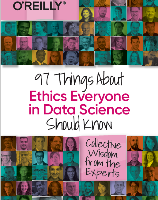
[New Book] 97 Things about Data Ethics in Data Science – Collective Wisdom from the Experts
 Some months ago I was approached about being part and contributing to a new book on Data Ethics for Data Science. It is now available to purchase on Amazon (and elsewhere), and this book now becomes the Sixth book that I’ve either solely or co-written. Check out my all my books here.
This has been an area I’ve been working in for some time now, in both research and assisting companies. I was able to make a couple of contributions to this book, and there has been great contributions from (other) global experts in Data Science and Data Ethics, and has been edited by Bill Franks.
Most of the high-profile cases of real or perceived unethical activity in data science aren’t matters of bad intent. Rather, they occur because the ethics simply aren’t thought through well enough. Being ethical takes constant diligence, and in many situations identifying the right choice can be difficult.
In this in-depth book, contributors from top companies in technology, finance, and other industries share experiences and lessons learned from collecting, managing, and analyzing data ethically. Data science professionals, managers, and tech leaders will gain a better understanding of ethics through powerful, real-world best practices.
The book is available in paper back and kindle formats and is published by O’Reilly Press.
You might be interested in my previous book on Data Science, part of the MIT Press Essentials Series. This book has been a Best Seller in 2018 and 2019 on Amazon.

Partitioned Models – Oracle Machine Learning (OML)
Building machine learning models can be a relatively trivial task. But getting to that point and understanding what to do next can be challenging. Yes the task of creating a model is simple and usually takes a few line of code. This is what is shown in most examples. But when you try to apply to real world problems we are faced with other challenges. Some of which include volume of data is larger, building efficient ML pipelines is challenging, time to create models gets longer, applying models to new data in real-time takes longer (not possible in real-time), etc. Yes these are typically challenges and most of these can be easily overcome.
When building ML solutions for real-world problem you will be faced with building (and deploying) many 10s or 100s of ML models. Why are so many models needed? Almost every example we see for ML takes the entire data set and build a model on that data. When you think about it, not everyone in the data set can be considered in the same grouping (similar characteristics). If we were to build a model on the data set and apply it to new data, we will get a generic prediction. A prediction comparing the new data item (new customer, purchase, etc) with everyone else in the data population. Maybe this is why so many ML project fail as they are building generic solution that performs badly when run on new (and evolving) data.
To overcome this we start to look at the different groups of data in the data set. Can the data set be divided into a number of different parts based on some characteristics. If we could do this and build a separate model on each group (or cluster), then we would have ML models that would be more accurate with their predictions. This is where we will end up creating 10s or 100s of models. As you can imagine the work involved in doing this with be LOTs. Then think about all the coding needed to manage all of this. What about the complexity of all the code needed for making the predictions on new data.
Yes all of this gets complex very, very quickly!
Ideally we want a separate model for each group
But how can you do that efficiently? is it possible?
When working with Oracle Machine Learning, you can use a feature called partitioned models. Partitioned Models are designed to handle this type of problem. They are designed to:
- make the building of models simple
- scales as the data and number of partitions increase
- includes all the steps part of the ML pipeline (all the data prep, transformations, etc)
- make predicting new data using the ML model simple
- make the deployment of the ML model easy
- make the MLOps process simple
- make the use of ML model easy to use by all developers no matter the programming language
- make the ML model build and ML model scoring quick and with better, more accurate predictions.

Let us work through an example. In this example lets start by creating a Random Forest ML model using the entire data set. The following code shows setting up the Parameters settings table. The second code segment creates the Random Forest ML model. The training data set being used in this example contains 72,000 records.
BEGIN
  DELETE FROM BANKING_RF_SETTINGS;

  INSERT INTO banking_RF_settings (setting_name, setting_value)
  VALUES (dbms_data_mining.algo_name, dbms_data_mining.algo_random_forest);

  INSERT INTO banking_RF_settings (setting_name, setting_value)
  VALUES (dbms_data_mining.prep_auto, dbms_data_mining.prep_auto_on);

 COMMIT;
END;
/

-- Create the ML model
DECLARE
   v_start_time  TIMESTAMP;
BEGIN
   DBMS_DATA_MINING.DROP_MODEL('BANKING_RF_72K_1');

   v_start_time := current_timestamp;

   DBMS_DATA_MINING.CREATE_MODEL(
      model_name          => 'BANKING_RF_72K_1',
      mining_function     => dbms_data_mining.classification,
      data_table_name     => 'BANKING_72K',
      case_id_column_name => 'ID',
      target_column_name  => 'TARGET',
      settings_table_name => 'BANKING_RF_SETTINGS');

   dbms_output.put_line('Time take to create model = ' || to_char(extract(second from (current_timestamp-v_start_time))) || ' seconds.');
END;
/
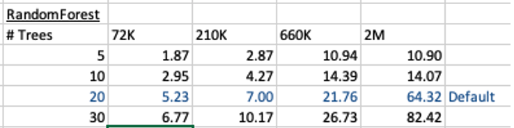
This is the basic setup and the following table illustrates how long the CREATE_MODEL function takes to run for different sizes of training datasets and with different number of trees per model. The default number of trees is 20.
To run this model against new data we could use something like the following SQL query.
SELECT cust_id, target,
       prediction(BANKING_RF_72K_1 USING *)  predicted_value,
       prediction_probability(BANKING_RF_72K_1 USING *) probability
FROM   bank_test_v;
This is simple and straight forward to use.
For the 72,000 records it takes just approx 5.23 seconds to create the model, which includes creating 20 Decision Trees. As mentioned earlier, this will be a generic model covering the entire data set.
To create a partitioned model, we can add new parameter which lists the attributes to use to partition the data set. For example, if the partition attribute is MARITAL, we see it has four different values. This means when this attribute is used as the partition attribute, Oracle Machine Learning will create four separate sub Random Forest models all until the one umbrella model. This means the above SQL query to run the model, does not change and the correct sub model will be selected to run on the data based on the value of MARITAL attribute.
To create this partitioned model you need to add the following to the settings table.
BEGIN
  DELETE FROM BANKING_RF_SETTINGS;

  INSERT INTO banking_RF_settings (setting_name, setting_value)
  VALUES (dbms_data_mining.algo_name, dbms_data_mining.algo_random_forest);

  INSERT INTO banking_RF_settings (setting_name, setting_value)
  VALUES (dbms_data_mining.prep_auto, dbms_data_mining.prep_auto_on);

  INSERT INTO banking_RF_settings (setting_name, setting_value)
  VALUES (dbms_data_mining.odms_partition_columns, 'MARITAL’);

COMMIT;
END;
/
The code to create the model remains the same!
The code to call and use the model remains the same!
This keeps everything very simple and very easy to use.
When I ran the CREATE_MODEL code for the partitioned model, it took approx 8.3 seconds to run. Yes it took slightly longer than the previous example, but this time it is creating four models instead of one. This is still very quick!
What if I wanted to add more attributes to the partition key? Yes you can do that. The more attributes you add, the more sub-models will be be created.
For example, if I was to add JOB attribute to the partition key list. I will now get 48 sub-models (with 20 Decision Trees each) being created. The JOB attribute has 12 distinct values, multiplied by the 4 values for MARITAL, gives us 48 models.
INSERT INTO banking_RF_settings (setting_name, setting_value)
VALUES (dbms_data_mining.odms_partition_columns, 'MARITAL,JOB');
How long does this take the CREATE_MODEL code to run? approx 37 seconds!
Again that is quick!
Again remember the code to create the model and to run the model to predict on new data does not change. This means our applications using this ML model does not change. This shows us we can very easily increase the predictive accuracy of our models with only adding one additional model, and by improving this accuracy by adding more attributes to the partition key.
But you do need to be careful with what attributes to include in the partition key. If the attributes have a very high number of distinct values, will result in 100s, or 1000s of sub models being created.
An important benefit of using partitioned models is when a new distinct value occurs in one of the partition key attributes. You code to create the parameters and models does not change. OML will automatically will pick this up and do all the work under the hood.
GoLang – Consuming Oracle REST API from an Oracle Cloud Database)
Does anyone write code to access data in a database anymore, and by code I mean SQL? The answer to this question is ‘It Depends’, just like everything in IT.
Using REST APIs is very common for accessing processing data with a Database. From using an API to retrieve data, to using a slightly different API to insert data, and using other typical REST functions to perform your typical CRUD operations. Using REST APIs allows developers to focus on write efficient applications in a particular application, instead of having to swap between their programming language and SQL. In later cases most developers are not expert SQL developer or know how to work efficiently with the data. Therefore leave the SQL and procedural coding to those who are good at that, and then expose the data and their code via REST APIs. The end result is efficient SQL and Database coding, and efficient application coding. This is a win-win for everyone.
I’ve written before about creating REST APIs in an Oracle Cloud Database (DBaaS and Autonomous). In these writings I’ve shown how to use the in-database machine learning features and to use REST APIs to create an interface to the Machine Learning models. These models can be used to to score new data, making a machine learning prediction. The data being used for the prediction doesn’t have to exist in the database, instead the database is being used as a machine learning scoring engine, accessed using a REST API.
In that article I showed how easy it was to use the in-database machine model using Python.
Python has a huge fan and user base, but some of the challenges with Python is with performance, as it is an interrupted language. Don’t get be wrong on this, as lots of work has gone into making Python more efficient. But in some scenarios it just isn’t fast enough. In does scenarios people will switch into using other quicker to execute languages such as C, C++, Java and GoLang.
Here is the GoLang code to call the in-database machine learning model and process the returned data.
import (
    "bytes"
    "encoding/json"
    "fmt"
    "io/ioutil"
    "net/http"
    "os"
)

func main() {
    fmt.Println("---------------------------------------------------")
    fmt.Println("Starting Demo - Calling Oracle in-database ML Model")
    fmt.Println("")

    // Define variables for REST API and parameter for first prediction
    rest_api = "<full REST API>"

    // This wine is Bad
    a_country := "Portugal"
    a_province := "Douro"
    a_variety := "Portuguese Red"
    a_price := "30"

    // call the REST API adding in the parameters
    response, err := http.Get(rest_api +"/"+ a_country +"/"+ a_province +"/"+ a_variety +"/"+ a_price)
    if err != nil {
        // an error has occurred. Exit
        fmt.Printf("The HTTP request failed with error :: %s\n", err)
        os.Exit(1)
    } else {
        // we got data! Now extract it and print to screen
        responseData, _ := ioutil.ReadAll(response.Body)
        fmt.Println(string(responseData))
    }
    response.Body.Close()

    // Lets do call it again with a different set of parameters

    // This wine is Good - same details except the price is different
    a_price := "31"

    // call the REST API adding in the parameters
    response, err := http.Get(rest_api +"/"+ a_country +"/"+ a_province +"/"+ a_variety +"/"+ a_price)
    if err != nil {
        // an error has occurred. Exit
        fmt.Printf("The HTTP request failed with error :: %s\n", err)
        os.Exit(1)
    } else {
        responseData, _ := ioutil.ReadAll(response.Body)
        fmt.Println(string(responseData))
    }
    defer response.Body.Close()

    // All done!
    fmt.Println("")
    fmt.Println("...Finished Demo ...")
    fmt.Println("---------------------------------------------------")
}

You must be logged in to post a comment.