
SQL
Valintine’s Day SQL
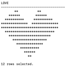
Well today is February 14th and is know as (St.) Valintine’s Day. Here is a piece of SQL I just put together to mark today. Enjoy and Happy St. Valintine’s Day.
WITH heart_top(lev, love) AS (
   SELECT 1 lev, RPAD(' ', 7, ' ') || '**          **' love
   FROM dual
   UNION ALL
   SELECT heart_top.lev+1,
          RPAD(' ', 6-heart_top.lev*2, ' ') ||
          RPAD('*', (heart_top.lev*4)+2, '*') ||
          RPAD(' ', 11-heart_top.lev*3, ' ') ||
          RPAD('*', (heart_top.lev*4)+2, '*')  love
   FROM heart_top
   WHERE heart_top.lev < 4
),
   heart_bottom(lev, love) AS (
     SELECT 1 lev, '******************************' love
     FROM dual
     UNION ALL
     SELECT heart_bottom.lev+1,
          RPAD(' ', heart_bottom.lev*2, ' ') ||
          RPAD('*', 15-heart_bottom.lev*2, '*') ||
          RPAD('*', 15-heart_bottom.lev*2, '*')  love
     FROM heart_bottom
     WHERE heart_bottom.lev < 8
)
SELECT love FROM heart_top
union all
SELECT love FROM heart_bottom;
Which gives us the following.
Bid you know : St. Valentine, the patron saint of love, was executed in Rome and buried there in the 3rd century. In 1835, an Irish priest was granted permission to exhume his remains, and now his skeleton lies in Whitefriar Church in Dublin city center.

Using SQL to create some festive Christmas Trees
Here are a few examples I found on the “great internet” of how SQL can be used to create some festive Christmas cheer and fun. See links to the original posts. Most of the examples shown below have been run on Oracle 21c Docker image, or on SQL Server or MySQL.
Our first example comes from Gerald Venzi who posted this on twitter. See later in the post for Christmas trees created using similar SQL queries.
WITH tree(lev, xmas) AS (
   SELECT 1 lev, RPAD(' ', 10, ' ') || '*' xmas
   FROM dual
   UNION ALL
   SELECT tree.lev+1,
          RPAD(' ', 10-tree.lev, ' ') ||
             RPAD('^', tree.lev+1, '^') ||
             LPAD('^', tree.lev, '^')  xmas
   FROM tree
   WHERE tree.lev < 10
)
SELECT '    Merry Christmas!' AS "Merry Christmas!" FROM dual
UNION ALL
SELECT xmas FROM TREE
UNION ALL
SELECT '         | |' FROM dual
UNION ALL
SELECT '      ~~/   \~~' FROM dual;
Our next example includes using Spatial Data on SQL Server to create a Christmas Tree. This example comes from Niket Kedia.
USE tempdb
GO

— Create a table

CREATE TABLE #xmasTREE (shape GEOMETRY )

–Creating the Christmas tree with stars

INSERT INTO #xmasTREE

VALUES
(‘POLYGON((4 0, 0 0, 4 2, 1 2, 4 4, 1 4, 4 6, 2 6, 5 10, 8 6, 6 6, 9 4, 6 4, 9 2, 6 2, 10 0, 4 0))’ ),
(‘POLYGON((3.5 0, 4 -1, 6 -1, 6.5 0, 3.5 0))’ ),
(‘POLYGON((5 9.5, 4.5 9.25, 4.6 9.9, 4.1 10.2, 4.8 10.2, 5 10.9, 5.2 10.2, 5.9 10.2, 5.4 9.9, 5.5 9.25, 5 9.5))’ ),
(‘POLYGON((2 5.5, 1.5 5.25, 1.6 5.9, 1.1 6.2, 1.8 6.2, 2 6.9, 2.2 6.2, 2.9 6.2, 2.4 5.9, 2.5 5.25, 2 5.5))’ ),
(‘POLYGON((8 5.5, 7.5 5.25, 7.6 5.9, 7.1 6.2, 7.8 6.2, 8 6.9, 8.2 6.2, 8.9 6.2, 8.4 5.9, 8.5 5.25, 8 5.5))’ ),
(‘POLYGON((1 3.5, 0.5 3.25, 0.6 3.9, 0.1 4.2, 0.8 4.2, 1 4.9, 1.2 4.2, 1.9 4.2, 1.4 3.9, 1.5 3.25, 1 3.5))’ ),
(‘POLYGON((9 3.5, 8.5 3.25, 8.6 3.9, 8.1 4.2, 8.8 4.2, 9 4.9, 9.2 4.2, 9.9 4.2, 9.4 3.9, 9.5 3.25, 9 3.5))’ ), (‘POLYGON((1 1.5, 0.5 1.25, 0.6 1.9, 0.1 2.2, 0.8 2.2, 1 2.9, 1.2 2.2, 1.9 2.2, 1.4 1.9, 1.5 1.25, 1 1.5))’ ), (‘POLYGON((9 1.5, 8.5 1.25, 8.6 1.9, 8.1 2.2, 8.8 2.2, 9 2.9, 9.2 2.2, 9.9 2.2, 9.4 1.9, 9.5 1.25, 9 1.5))’ ),
(‘POLYGON((0 -0.5, -0.5 -0.75, -0.4 -0.1, -0.9 0.2, -0.2 0.2, 0 0.9, 0.2 0.2, 0.9 0.2, 0.4 -0.1, 0.5 -0.75, 0 -0.5))’ ),
(‘POLYGON((10 -0.5, 9.5 -0.75, 9.6 -0.1, 9.1 0.2, 9.8 0.2, 10 0.9, 10.2 0.2, 10.9 0.2, 10.4 -0.1, 10.5 -0.75, 10 -0.5))’ ),
(‘POLYGON((5 -2, 4.5 -2, 4.5 -1, 5 -1, 5.5 -1, 5.5 -2, 5 -2))’)

–Create the “Merry Christmas” greetings

INSERT INTO #xmasTREE

VALUES (‘POLYGON((-2 11, -2 12, -1.75 12, -1.5 11.5, -1.25 12, -1 12, -1 11, -1.25 11, -1.25 11.7, -1.5 11.2, -1.75 11.7, -1.75 11, -2 11))’ ),–M
(‘POLYGON((-1 11, -1 12, 0 12, 0 11.8, -0.75 11.8, -0.75 11.6, -0.25 11.6, -0.25 11.4, -0.75 11.4, -0.75 11.2, 0 11.2, 0 11, -1 11))’ ),–E
(‘POLYGON((0 11, 0 12, 1 12, 1 11.5, 0.4 11.5, 1 11, 0.7 11, 0.2 11.4, 0.2 11, 0 11),(0.2 11.8, 0.8 11.8, 0.8 11.7, 0.2 11.7, 0.2 11.8))’ ),–R
(‘POLYGON((1 11, 1 12, 2 12, 2 11.5, 1.4 11.5, 2 11, 1.7 11, 1.2 11.4, 1.2 11, 1 11),(1.2 11.8, 1.8 11.8, 1.8 11.7, 1.2 11.7, 1.2 11.8))’ ),–R
(‘POLYGON((2 12, 2.2 12, 2.5 11.6, 2.8 12, 3 12, 2.6 11.5, 2.6 11, 2.4 11, 2.4 11.5, 2 12))’ ), –Y
(‘POLYGON((4 11, 4 12, 5 12, 5 11.8, 4.25 11.8, 4.25 11.2, 5 11.2, 5 11, 4 11))’ ),–C
(‘POLYGON((5 11, 5 12, 5.2 12, 5.2 11.6, 5.8 11.6, 5.8 12, 6 12, 6 11, 5.8 11, 5.8 11.4, 5.2 11.4, 5.2 11, 5 11))’ ),–H
(‘POLYGON((6 11, 6 12, 7 12, 7 11.5, 6.4 11.5, 7 11, 6.7 11, 6.2 11.4, 6.2 11, 6 11),(6.2 11.8, 6.8 11.8, 6.8 11.7, 6.2 11.7, 6.2 11.8))’ ),–R
(‘POLYGON((7.2 11, 7.2 11.2, 7.4 11.2, 7.4 11.8, 7.2 11.8, 7.2 12, 7.8 12, 7.8 11.8, 7.6 11.8, 7.6 11.2, 7.8 11.2, 7.8 11, 7.2 11))’ ),–I
(‘POLYGON((8 11, 8 11.2, 8.8 11.2, 8.8 11.4, 8 11.4, 8 12, 9 12, 9 11.8, 8.2 11.8, 8.2 11.6, 9 11.6, 9 11, 8 11))’ ),–S
(‘POLYGON((9 11.8, 9 12, 10 12, 10 11.8, 9.6 11.8, 9.6 11, 9.4 11, 9.4 11.8, 9 11.8))’ ),–T
(‘POLYGON((10 11, 10 12, 10.25 12, 10.5 11.5, 10.75 12, 11 12, 11 11, 10.75 11, 10.75 11.7, 10.5 11.2, 10.25 11.7, 10.25 11, 10 11))’ ),–M
(‘POLYGON((11 11, 11 12, 12 12, 12 11, 11.75 11, 11.75 11.3, 11.25 11.3, 11.25 11, 11 11),(11.25 11.5, 11.25 11.8, 11.75 11.8, 11.75 11.5, 11.25 11.5))’ ),–A
(‘POLYGON((12 11, 12 11.2, 12.8 11.2, 12.8 11.4, 12 11.4, 12 12, 13 12, 13 11.8, 12.2 11.8, 12.2 11.6, 13 11.6, 13 11, 12 11))’ )–S

–Decorate the tree with some round bell circles

DECLARE @counter INT = 0

,@x INT

,@y INT ;

WHILE ( @counter < 25 )

BEGIN

INSERT INTO #xmasTREE

VALUES (GEOMETRY::Point(RAND() * 5 + 2.5, RAND() * 8.5, 0).STBuffer(0.3) )

SET @counter+=1 ;

END

Select * from #xmasTREE
Drop table #xmasTREE
Our next example comes from StackOverflow with a similar example for MySQL.
DECLARE @g TABLE (g GEOMETRY, ID INT IDENTITY(1,1));


-- Adjust Color

INSERT INTO @g(g) SELECT TOP 29 CAST('POLYGON((0 0, 0 0.0000001, 0.0000001 0.0000001, 0 0))' as geometry) FROM sys.messages;

-- Build Christmas Tree

INSERT INTO @g(g) VALUES (CAST('POLYGON((0 0,900 0,450 400, 0 0 ))' as geometry).STUnion(CAST('POLYGON((80 330,820 330,450 640,80 330 ))' as geometry)).STUnion(CAST('POLYGON((210 590,690 590,450 800, 210 590 ))' as geometry)));

-- Adjust Color

INSERT INTO @g(g) SELECT TOP 294 CAST('POLYGON((0 0, 0 0.0000001, 0.0000001 0.0000001, 0 0))' as geometry) FROM sys.messages;

-- Build a Star

INSERT INTO @g(g) VALUES (CAST('POLYGON ((450 910, 465.716 861.631, 516.574 861.631, 475.429 831.738, 491.145 783.369, 450 813.262, 408.855 783.369, 424.571 831.738, 383.426 861.631, 434.284 861.631, 450 910))' as geometry));

-- Build Colored Balls

INSERT INTO @g(g) SELECT TOP 2 CAST('POLYGON((0 0, 0 0.0000001, 0.0000001 0.0000001, 0 0))' as geometry) FROM sys.messages;

INSERT INTO @g(g) VALUES (CAST('CURVEPOLYGON (CIRCULARSTRING (80 290, 110 320, 140 290, 110 260, 80 290))' as geometry));

INSERT INTO @g(g) SELECT TOP 2 CAST('POLYGON((0 0, 0 0.0000001, 0.0000001 0.0000001, 0 0))' as geometry) FROM sys.messages;

INSERT INTO @g(g) VALUES (CAST('CURVEPOLYGON (CIRCULARSTRING (760 290, 790 320, 820 290, 790 260, 760 290))' as geometry));

INSERT INTO @g(g) SELECT TOP 3 CAST('POLYGON((0 0, 0 0.0000001, 0.0000001 0.0000001, 0 0))' as geometry) FROM sys.messages;

INSERT INTO @g(g) VALUES (CAST('CURVEPOLYGON (CIRCULARSTRING (210 550, 240 580, 270 550, 240 520, 210 550))' as geometry));

INSERT INTO @g(g) SELECT TOP 46 CAST('POLYGON((0 0, 0 0.0000001, 0.0000001 0.0000001, 0 0))' as geometry) FROM sys.messages;

INSERT INTO @g(g) VALUES (CAST('CURVEPOLYGON (CIRCULARSTRING (630 550, 660 580, 690 550, 660 520, 630 550))' as geometry));


SELECT g FROM @g ORDER BY ID;

GO
Connor McDonold posted the following SQL to create a Christmas Tree on StackOverflow in 2020, and wrote a blog post for it in December 2021. I just made one very very minor change to it.
You need to be careful where you run this. It runs best on/in a Linux environment, docker, VM, etc using SQL Command Line or SQL*Plus. For me, SQL Developer struggled to present the results correctly.
select replace(replace(replace(r,'X',chr(27)||'[42m'||chr(27)||'[1;'||to_char(32)||'m'||'X'||chr(27)||'[0m'),
    'T',chr(27)||'[43m'||chr(27)||'[1;'||to_char(33)||'m'||'T'||chr(27)||'[0m'),
    '@',chr(27)||'[33m'||chr(27)||'[1;'||to_char(31)||'m'||'@'||chr(27)||'[0m')  Happy_Christmas
from ( select lpad(' ',20-e-i)|| case when dbms_random.value < 0.3 then substr(s,1,e*2-3+i*2)
       else substr(substr(s,1,dbms_random.value(1,e*2-3+i*2-1))||'@'||s,1,e*2-3+i*2) end r
from ( select rpad('X',40,'X') s,rpad('T',40,'T') t from dual ) ,
( select level i, level+2 hop from dual connect by level <= 4 ) , lateral
( select level e from dual connect by level <= hop ) union all select lpad(' ',17)||substr(t,1,3)
from ( select rpad('X',40,'X') s,rpad('T',40,'T') t from dual ) connect by level <= 5 );
Next up we have a simpler Christmas Tree. This comes from Matheus Boesing and his original post on grepora.
clear screen
set feedback off;
set heading off;
set pages 80;
SELECT DECODE(SIGN(FLOOR(maxwidth / 2) - ROWNUM),
              1,
              LPAD(' ', FLOOR(maxwidth / 2) - (ROWNUM - 1)) ||
              RPAD('*', 2 * (ROWNUM - 1) + 1, ' *'),
              LPAD('* * *', FLOOR(maxwidth / 2) + 3))
  FROM all_objects, (SELECT 40 AS maxwidth FROM DUAL)
 WHERE ROWNUM < FLOOR(maxwidth / 2) + 5
union all select '     Happy Christmas from Brendan!' from dual;
set heading on;
set feedback on;
This next example comes from LearnSQL and is similar to the previous example, but this time we get a multiple trees.
clear screen
set feedback off;
set heading off;
set pages 80;
WITH small_tree(tree_depth,pine) AS (
  SELECT 1 tree_depth,
  rpad(' ',10,' ') || '*'
  || rpad(' ',20,' ') || '*'
  || rpad(' ',20,' ') || '*'
  pine
  FROM   dual
  UNION ALL
  SELECT small_tree.tree_depth +1 tree_depth,
  rpad(' ',10-small_tree.tree_depth,' ') || rpad('*',small_tree.tree_depth+1,'.') || lpad('*',small_tree.tree_depth,'.')
  || rpad(' ',20-small_tree.tree_depth-tree_depth,' ') || rpad('*',small_tree.tree_depth+1,'.') || lpad('*',small_tree.tree_depth,'.')
  || rpad(' ',20-small_tree.tree_depth-tree_depth,' ') || rpad('*',small_tree.tree_depth+1,'.') || lpad('*',small_tree.tree_depth,'.') pine
  FROM   small_tree
  where small_tree.tree_depth < 10
)
SELECT   rpad(' ',9,' ') ||'Ho'
         || rpad(' ',19,' ') || 'Ho'
         || rpad(' ',19,' ') || 'Ho'
  pine
  FROM   dual
  UNION ALL
SELECT pine
FROM small_tree;
set heading on;
set feedback on;
Hans Viehmann from the Oracle Spatial teams sent me this example using Oracle Spatial and Oracle Spatial Studio. The geospatial data is defined using GeoJSON. The funny coordinates are referencing the Santa Claus village near Rovaniemi in Finnish Lappland, right on the Arctic Circle. Oracle Spatial Studio can be used to view the Christmas tree on a map (see image below).
DROP TABLE XMAS_TREE_JSON;

DROP TABLE XMAS_TREE;

CREATE TABLE XMAS_TREE_JSON (
    ID   NUMBER(10),
    DATA CLOB,
    CONSTRAINT XMAS_TREE_PK PRIMARY KEY ( ID ),
    CONSTRAINT XMAS_TREE_JSON_CHK CHECK ( DATA IS JSON )
);

INSERT INTO XMAS_TREE_JSON VALUES (
    1,
    '{
      "type": "Feature",
      "properties": { "label": "Tree"},
      "geometry": {
        "type": "Polygon",
        "coordinates": [
          [[25.84725335240364,
              66.5437744044363],
            [25.847166180610653,
              66.543721555766],
            [25.847235918045044,
              66.5437231572425],
            [25.84712728857994,
              66.5436740452493],
            [25.84722116589546,
              66.54367564672889],
            [25.847095102071762,
              66.54362012871027],
            [25.847205072641373,
              66.54362226402098],
            [25.847202390432358,
              66.54361105363778],
            [25.847297608852386,
              66.54361212129352],
            [25.847297608852386,
              66.5436238655039],
            [25.84740623831749,
              66.5436243993315],
            [25.84728017449379,
              66.54367724820834],
            [25.84736466407776,
              66.54367724820834],
            [25.847273468971252,
              66.54372369106797],
            [25.847321748733517,
              66.54372369106797],
            [25.84725335240364,
              66.5437744044363]
          ]
        ]
      }
    }'
);

COMMIT;

CREATE TABLE XMAS_TREE
    AS
        SELECT
            ID,
            JSON_VALUE(DATA, '$.geometry' RETURNING SDO_GEOMETRY) AS SHAPE,
            JSON_VALUE(DATA, '$.properties.label')                AS LABEL
        FROM
            XMAS_TREE_JSON;
Happy Christmas everyone.
Measuring Kurtosis of Data in Oracle (21c)
Kurtosis is a new analytics function in Oracle 21c (20c) and is one of a set of commonly used statistical functions used to evaluate data to see and understand the behavior of the data.
[See my previous post where I give examples of the new Skewness functions]
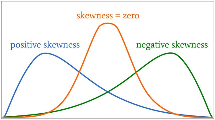
Kurtosis is the measurement of the tails of the data distribution and its comparison with that of normal distribution. The Kurtosis of the normal distribution is said to be 3. To make interpenetrating results easier (a Zero) kurtosis measure for gaussian/normal distribution by subtracting 3 from its value, this is called Excess Kurtosis. Kurtosis can be used to describe the height or the breath of the distributions, when compared to a normal distributions, although this is not theoretically correct, it gives a simpler explanation and visualization of it. The following diagram gives an example of a normal distribution, a plot of Positive Kurtosis and Negative Kurtosis.

Prior to the new Kurtosis SQL functions (KURTOSIS_POP and KURTOSIS_SAMP), you had to calculate the Kurtosis value manually using something like the following SQL. These use the same data and attributes set used for the Skewness examples.
select avg(KV) K_value
from (select power((age - avg(age) over ())/stddev(age) over (), 4) KV
      from cust_data)
union all
select avg(KV) K_value
from (select power((duration - avg(duration) over ())/stddev(duration) over (), 4) KV
      from cust_data);

K_value
------------------------------------------
3.79088571963003808388287765230733611415
23.24420570926391173498028369605428048285
These don’t include the subtraction of 3 to give a zero kurtosis, and these values can be compared to the data distribution charts shown in the Skewness post.
Now with the new Kurtosis functions it simplifies the tasks of getting these values.
SELECT kurtosis_pop(age), kurtosis_samp(age)
FROM bank_additional
union all
SELECT kurtosis_pop(duration), kurtosis_samp(duration)
FROM bank_additional;

KURTOSIS_POP         KURTOSIS_SAMP
------------------   -----------------------------------------
 0.791069803527387    0.79131153115443467194451597661213420763
20.245334438614832   20.24793801497878942299945619307526969226
As you can see the Kurtosis function have the subtraction include.
As with the Skewness functions, the SAMP version works on a sample of the data values and as the number inputs increases, and differences between the POP and SAMP will reduce.
Measuring Skewness of Data in Oracle (21c)
When analyzing data you will look at using a variety of different statistical functions to explore variable data insights.
One of these is the Skewness of the data.
Skewness is a measure of the asymmetry of the probability distribution about its mean. This looks a the tail of the data, with a positive value indicating the tail on the right side of the distribution, and a negative value when the tail is on the left hand side. A zero value indicates the tails on both side balance out, as shown in the following image.
Most SQL dialects support Skewness using with an inbuilt function. But if it doesn’t then you would need to write your own version of the calculation, for example using the following.
SELECT avg(SV) S_value
FROM   (SELECT  power((age – avg(age) over ())/stddev(age) over (), 3) SV
        FROM    cust_data)
Here are charts illustrating the data in my table. These include the distributions for the AGE and DURATION attributes.
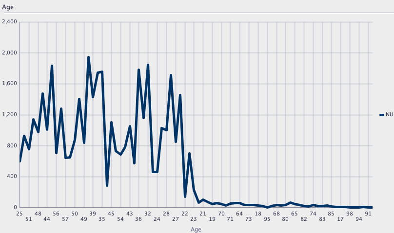

We can see the data is skewed. When we run the above code we get the following values.
Age = 0.78
Duration = 3.26
We can see the skewness of Duration is significantly longer, giving a positive value as the skewness is to the right.
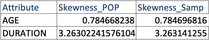
In Oracle 21s we now have new Skewness functions called SKEWNESS_POP and SKEWNESS_SAMP. The POP version of the function considers all records, where as the SAMP function considers a sample of the records. When your data set grows into many millions of records the SKEWNESS_SAMP will give a quicker response as it works with a sample of the data set
Both functions will give similar values but at the number of input records the returned values will returned will converge.
SELECT skewness_pop(age), skewness_samp(age)
FROM cust_data;
SELECT skewness_pop(duration), skewness_samp(duration)
FROM cust_data;
Adding Text Processing to Classification Machine Learning in Oracle Machine Learning
One of the typical machine learning functions is Classification. This is in widespread use across most domains and geographic regions. I’ve written several blog posts on this topic over many years (and going back many, many year) on how to do this using Oracle Machine Learning (OML) (formally known as Oracle Advanced Analytic and in the Oracle Data Miner tool in SQL Developer). Just do a quick search of my blog to find some of these posts.
When it comes to Classification problems, typically the data set will be contain your typical categorical and numerical variables/features. The Automatic Data Preparation (ADP) feature of OML where it automatically pre-processes and transforms these variable for input to the machine learning algorithm. This greatly reduces the boring work of the data scientist and increases their productivity.
But sometimes data sets come with text descriptions. These will contain production descriptions, free format text, and other descriptive data, for example product reviews. But how can this information be included as part of the input data set to the machine learning algorithms. Oracle allows this kind of input data, and a letting bit of setup is needed to tell Oracle how to process the data set. This uses the in-database feature of Oracle Text.
The following example walks through an example of the steps needed to pre-process and include the text processing as part of the machine learning algorithm.
The data set: The data used to illustrate this and to show the steps needed, is a data set from Kaggle webiste. This data set contains 130K Wine Reviews. This data set contain descriptive information of the wine with attributes about each wine including country, region, number of points, price, etc as well as a text description contain a review of the wine.
The following are 2 files containing the DDL (to create the table) and then Import the data set (using sql script with insert statements). These can be run in your schema (in order listed below).
I’ll leave the Data Exploration to you to do and to discover some early insights.
The ML Question
I want to be able to predict if a wine is a good quality wine, based on the prices and different characteristics of the wine?
Data Preparation
To be able to answer this question the first thing needed is to define a target variable to identify good and bad wines. To do this create a new attribute/feature called POINTS_BIN and populate it based on the number of points a wine has. If it has >90 points it is a good wine, if <90 points it is a bad wine.
ALTER TABLE WineReviews130K_bin ADD POINTS_BIN VARCHAR2(15);

UPDATE WineReviews130K_bin
SET POINTS_BIN = 'GT_90_Points'
WHERE winereviews130k_bin.POINTS >= 90;

UPDATE WineReviews130K_bin
SET POINTS_BIN = 'LT_90_Points'
WHERE winereviews130k_bin.POINTS < 90;

alter table WineReviews130K_bin DROP COLUMN POINTS;
The DESCRIPTION column data type needs to be changed to CLOB. This is to allow the Text Mining feature to work correctly.
-- add a new column of data type CLOB
ALTER TABLE WineReviews130K_bin ADD (DESCRIPTION_NEW CLOB);

-- update new column with data from the DESCRIPTION attribute
UPDATE WineReviews130K_bin SET DESCRIPTION_NEW = DESCRIPTION;

-- drop the DESCRIPTION attribute from table
ALTER TABLE WineReviews130K_bin DROP COLUMN DESCRIPTION;

-- rename the new attribute to replace DESCRIPTION
ALTER TABLE WineReviews130K_bin RENAME COLUMN DESCRIPTION_NEW TO DESCRIPTION;
Text Mining Configuration
There are a number of things we need to define for the Text Mining to work, these include a Lexer, Stop Word list and preferences.
First define the Lexer to use. In this case we will use a basic one and basic settings
BEGIN
   ctx_ddl.create_preference('mylex', 'BASIC_LEXER');
   ctx_ddl.set_attribute('mylex', 'printjoins', '_-');
   ctx_ddl.set_attribute ( 'mylex', 'index_themes', 'NO');
   ctx_ddl.set_attribute ( 'mylex', 'index_text', 'YES');
END;
Next we can define a Stop Word List. Oracle Text comes with a predefined set of Stop Word lists for most of the common languages. You can add to one of those list or create your own. Depending on the domain you are working in it might be easier to create your own and it is very straight forward to do. For example:
DECLARE
   v_stoplist_name varchar2(100);
BEGIN
   v_stoplist_name := 'mystop';
   ctx_ddl.create_stoplist(v_stoplist_name, 'BASIC_STOPLIST');
   ctx_ddl.add_stopword(v_stoplist_name, 'nonetheless');
   ctx_ddl.add_stopword(v_stoplist_name, 'Mr');
   ctx_ddl.add_stopword(v_stoplist_name, 'Mrs');
   ctx_ddl.add_stopword(v_stoplist_name, 'Ms');
   ctx_ddl.add_stopword(v_stoplist_name, 'a');
   ctx_ddl.add_stopword(v_stoplist_name, 'all');
   ctx_ddl.add_stopword(v_stoplist_name, 'almost');
   ctx_ddl.add_stopword(v_stoplist_name, 'also');
   ctx_ddl.add_stopword(v_stoplist_name, 'although');
   ctx_ddl.add_stopword(v_stoplist_name, 'an');
   ctx_ddl.add_stopword(v_stoplist_name, 'and');
   ctx_ddl.add_stopword(v_stoplist_name, 'any');
   ctx_ddl.add_stopword(v_stoplist_name, 'are');
   ctx_ddl.add_stopword(v_stoplist_name, 'as');
   ctx_ddl.add_stopword(v_stoplist_name, 'at');
   ctx_ddl.add_stopword(v_stoplist_name, 'be');
   ctx_ddl.add_stopword(v_stoplist_name, 'because');
   ctx_ddl.add_stopword(v_stoplist_name, 'been');
   ctx_ddl.add_stopword(v_stoplist_name, 'both');
   ctx_ddl.add_stopword(v_stoplist_name, 'but');
   ctx_ddl.add_stopword(v_stoplist_name, 'by');
   ctx_ddl.add_stopword(v_stoplist_name, 'can');
   ctx_ddl.add_stopword(v_stoplist_name, 'could');
   ctx_ddl.add_stopword(v_stoplist_name, 'd');
   ctx_ddl.add_stopword(v_stoplist_name, 'did');
   ctx_ddl.add_stopword(v_stoplist_name, 'do');
   ctx_ddl.add_stopword(v_stoplist_name, 'does');
   ctx_ddl.add_stopword(v_stoplist_name, 'either');
   ctx_ddl.add_stopword(v_stoplist_name, 'for');
   ctx_ddl.add_stopword(v_stoplist_name, 'from');
   ctx_ddl.add_stopword(v_stoplist_name, 'had');
   ctx_ddl.add_stopword(v_stoplist_name, 'has');
   ctx_ddl.add_stopword(v_stoplist_name, 'have');
   ctx_ddl.add_stopword(v_stoplist_name, 'having');
   ctx_ddl.add_stopword(v_stoplist_name, 'he');
   ctx_ddl.add_stopword(v_stoplist_name, 'her');
   ctx_ddl.add_stopword(v_stoplist_name, 'here');
   ctx_ddl.add_stopword(v_stoplist_name, 'hers');
   ctx_ddl.add_stopword(v_stoplist_name, 'him');
   ctx_ddl.add_stopword(v_stoplist_name, 'his');
   ctx_ddl.add_stopword(v_stoplist_name, 'how');
   ctx_ddl.add_stopword(v_stoplist_name, 'however');
   ctx_ddl.add_stopword(v_stoplist_name, 'i');
   ctx_ddl.add_stopword(v_stoplist_name, 'if');
   ctx_ddl.add_stopword(v_stoplist_name, 'in');
   ctx_ddl.add_stopword(v_stoplist_name, 'into');
   ctx_ddl.add_stopword(v_stoplist_name, 'is');
   ctx_ddl.add_stopword(v_stoplist_name, 'it');
   ctx_ddl.add_stopword(v_stoplist_name, 'its');
   ctx_ddl.add_stopword(v_stoplist_name, 'just');
   ctx_ddl.add_stopword(v_stoplist_name, 'll');
   ctx_ddl.add_stopword(v_stoplist_name, 'me');
   ctx_ddl.add_stopword(v_stoplist_name, 'might');
   ctx_ddl.add_stopword(v_stoplist_name, 'my');
   ctx_ddl.add_stopword(v_stoplist_name, 'no');
   ctx_ddl.add_stopword(v_stoplist_name, 'non');
   ctx_ddl.add_stopword(v_stoplist_name, 'nor');
   ctx_ddl.add_stopword(v_stoplist_name, 'not');
   ctx_ddl.add_stopword(v_stoplist_name, 'of');
   ctx_ddl.add_stopword(v_stoplist_name, 'on');
   ctx_ddl.add_stopword(v_stoplist_name, 'one');
   ctx_ddl.add_stopword(v_stoplist_name, 'only');
   ctx_ddl.add_stopword(v_stoplist_name, 'onto');
   ctx_ddl.add_stopword(v_stoplist_name, 'or');
   ctx_ddl.add_stopword(v_stoplist_name, 'our');
   ctx_ddl.add_stopword(v_stoplist_name, 'ours');
   ctx_ddl.add_stopword(v_stoplist_name, 's');
   ctx_ddl.add_stopword(v_stoplist_name, 'shall');
   ctx_ddl.add_stopword(v_stoplist_name, 'she');
   ctx_ddl.add_stopword(v_stoplist_name, 'should');
   ctx_ddl.add_stopword(v_stoplist_name, 'since');
   ctx_ddl.add_stopword(v_stoplist_name, 'so');
   ctx_ddl.add_stopword(v_stoplist_name, 'some');
   ctx_ddl.add_stopword(v_stoplist_name, 'still');
   ctx_ddl.add_stopword(v_stoplist_name, 'such');
   ctx_ddl.add_stopword(v_stoplist_name, 't');
   ctx_ddl.add_stopword(v_stoplist_name, 'than');
   ctx_ddl.add_stopword(v_stoplist_name, 'that');
   ctx_ddl.add_stopword(v_stoplist_name, 'the');
   ctx_ddl.add_stopword(v_stoplist_name, 'their');
   ctx_ddl.add_stopword(v_stoplist_name, 'them');
   ctx_ddl.add_stopword(v_stoplist_name, 'then');
   ctx_ddl.add_stopword(v_stoplist_name, 'there');
   ctx_ddl.add_stopword(v_stoplist_name, 'therefore');
   ctx_ddl.add_stopword(v_stoplist_name, 'these');
   ctx_ddl.add_stopword(v_stoplist_name, 'they');
   ctx_ddl.add_stopword(v_stoplist_name, 'this');
   ctx_ddl.add_stopword(v_stoplist_name, 'those');
   ctx_ddl.add_stopword(v_stoplist_name, 'though');
   ctx_ddl.add_stopword(v_stoplist_name, 'through');
   ctx_ddl.add_stopword(v_stoplist_name, 'thus');
   ctx_ddl.add_stopword(v_stoplist_name, 'to');
   ctx_ddl.add_stopword(v_stoplist_name, 'too');
   ctx_ddl.add_stopword(v_stoplist_name, 'until');
   ctx_ddl.add_stopword(v_stoplist_name, 've');
   ctx_ddl.add_stopword(v_stoplist_name, 'very');
   ctx_ddl.add_stopword(v_stoplist_name, 'was');
   ctx_ddl.add_stopword(v_stoplist_name, 'we');
   ctx_ddl.add_stopword(v_stoplist_name, 'were');
   ctx_ddl.add_stopword(v_stoplist_name, 'what');
   ctx_ddl.add_stopword(v_stoplist_name, 'when');
   ctx_ddl.add_stopword(v_stoplist_name, 'where');
   ctx_ddl.add_stopword(v_stoplist_name, 'whether');
   ctx_ddl.add_stopword(v_stoplist_name, 'which');
   ctx_ddl.add_stopword(v_stoplist_name, 'while');
   ctx_ddl.add_stopword(v_stoplist_name, 'who');
   ctx_ddl.add_stopword(v_stoplist_name, 'whose');
   ctx_ddl.add_stopword(v_stoplist_name, 'why');
   ctx_ddl.add_stopword(v_stoplist_name, 'will');
   ctx_ddl.add_stopword(v_stoplist_name, 'with');
   ctx_ddl.add_stopword(v_stoplist_name, 'would');
   ctx_ddl.add_stopword(v_stoplist_name, 'yet');
   ctx_ddl.add_stopword(v_stoplist_name, 'you');
   ctx_ddl.add_stopword(v_stoplist_name, 'your');
   ctx_ddl.add_stopword(v_stoplist_name, 'yours');
   ctx_ddl.add_stopword(v_stoplist_name, 'drink');
   ctx_ddl.add_stopword(v_stoplist_name, 'flavors');
   ctx_ddl.add_stopword(v_stoplist_name, '2020');
   ctx_ddl.add_stopword(v_stoplist_name, 'now');
END;
Next define the preferences for processing the Text, for example what Stop Word list to use, if Fuzzy match is to be used and what language to use for this, number of tokens/words to process and if stemming is to be used.
BEGIN
   ctx_ddl.create_preference('mywordlist', 'BASIC_WORDLIST');
   ctx_ddl.set_attribute('mywordlist','FUZZY_MATCH','ENGLISH');
   ctx_ddl.set_attribute('mywordlist','FUZZY_SCORE','1');
   ctx_ddl.set_attribute('mywordlist','FUZZY_NUMRESULTS','5000');
   ctx_ddl.set_attribute('mywordlist','SUBSTRING_INDEX','TRUE');
   ctx_ddl.set_attribute('mywordlist','STEMMER','ENGLISH');
END;
And the final step is to piece it all together by defining a new Text policy
BEGIN
   ctx_ddl.create_policy('my_policy', NULL, NULL, 'mylex', 'mystop', 'mywordlist');
END;
Define Settings for OML Model
We will create two models. An Attribute Importance model and a Classification model. The following defines the model parameters for each of these.
CREATE TABLE att_import_model_settings (setting_name varchar2(30), setting_value varchar2(30));
INSERT INTO att_import_model_settings (setting_name, setting_value)
VALUES (''ALGO_NAME'', ''ALGO_AI_MDL'');
INSERT INTO att_import_model_settings (setting_name, setting_value)
VALUES (''PREP_AUTO'', ''ON'');
INSERT INTO att_import_model_settings (setting_name, setting_value)
VALUES (''ODMS_TEXT_POLICY_NAME'', ''my_policy'');
INSERT INTO att_import_model_settings (setting_name, setting_value)
VALUES (''ODMS_TEXT_MAX_FEATURES'', ''3000'')';
CREATE TABLE wine_model_settings (setting_name varchar2(30), setting_value varchar2(30));
INSERT INTO wine_model_settings (setting_name, setting_value)
VALUES (''ALGO_NAME'', ''ALGO_RANDOM_FOREST'');
INSERT INTO wine_model_settings (setting_name, setting_value)
VALUES (''PREP_AUTO'', ''ON'');
INSERT INTO wine_model_settings (setting_name, setting_value)
VALUES (''ODMS_TEXT_POLICY_NAME'', ''my_policy'');
INSERT INTO wine_model_settings (setting_name, setting_value)
VALUES (''ODMS_TEXT_MAX_FEATURES'', ''3000'')';
Create the Training and Test data sets.
CREATE TABLE wine_train_data
AS SELECT id, country, description, designation, points_bin, price, province, region_1, region_2, taster_name, variety, title
FROM winereviews130k_bin
SAMPLE (60) SEED (1);
CREATE TABLE wine_test_data
AS SELECT id, country, description, designation, points_bin, price, province, region_1, region_2, taster_name, variety, title
FROM winereviews130k_bin
WHERE id NOT IN (SELECT id FROM wine_train_data);
All the set up is done, we can move onto the creating the machine learning models.
Create the OML Model (Attribute Importance & Classification)
We are going to create two models. The first is an Attribute Important model. This will look at the data set and will determine what attributes contribute most towards determining the target variable. As we are incorporting Texting Mining we will see what words/tokens from the DESCRIPTION attribute also contribute towards the target variable.
BEGIN
   DBMS_DATA_MINING.CREATE_MODEL(
      model_name          => 'GOOD_WINE_AI',
      mining_function     => DBMS_DATA_MINING.ATTRIBUTE_IMPORTANCE,
      data_table_name     => 'winereviews130k_bin',
      case_id_column_name => 'ID',
      target_column_name  => 'POINTS_BIN',
      settings_table_name => 'att_import_mode_settings');
END;
We can query the system views for Oracle ML to find out what are the important variables.
SELECT * FROM dm$vagood_wine_ai
ORDER BY attribute_rank;
Here is the listing of the top 15 most important attributes. We can see from the first 15 rows and looking under column ATTRIBUTE_SUBNAME, the words from the DESCRIPTION attribute that seem to be important and contribute towards determining the value in the target attribute.

At this point you might determine, based on domain knowledge, some of these words should be excluded as they are generic for the domain. In this case, go back to the Stop Word List and recreate it with any additional words. This can be repeated until you are happy with the list. In this example, WINE could be excluded by including it in the Stop Word List.
Run the following to create the Classification model. It is very similar to what we ran above with minor changes to the name of the model, the data mining function and the name of the settings table.
BEGIN
   DBMS_DATA_MINING.CREATE_MODEL(
      model_name          => 'GOOD_WINE_MODEL',
      mining_function     => DBMS_DATA_MINING.CLASSIFICATION,
      data_table_name     => 'winereviews130k_bin',
      case_id_column_name => 'ID',
      target_column_name  => 'POINTS_BIN',
      settings_table_name => 'wine_model_settings');
END;
Apply OML Model
The model can be applied in similar ways to any other ML model created using OML. For example the following displays the wine details along with the predicted points bin values (good or bad) and the probability score (<=1) of the prediction.
SELECT id, price, country, designation, province, variety, points_bin,
       PREDICTION(good_wine_mode USING *) pred_points_bin,
       PREDICTION_PROBABILITY(good_wine_mode USING *) prob_points_bin
FROM wine_test_data;
Enhanced Window Clause functionality in Oracle 21c (20c)
Updated: Changed 20c to Oracle 21c, as Oracle 20c Database never really existed 🙂
The Oracle Database has had advanced analytical functions for some time now and with each release we get to have some new additions or some enhancements to existing functionality.
One new enhancement, available and documented in 21c (not yet released at time of writing this), is changing in the way the Window Clause can be defined for analytic functions. Oracle 21c is available on Oracle Cloud as a pre-release for evaluation purposes (but it won’t be available for much longer!). The examples shown below are based on using this 21c pre-release of the database.
NOTE: At this point, no one really knows when or if 20c will be released. I’m sure all the documented 20c new features will be rolled into 21c, whenever that will be released.
Before giving some examples of the new Window Clause functionality, lets have a quick recap on how we could use it up to now (up to 19c database). Here is a simple example of windowing the data by creating partitions based on the distinct values in DEPTNO column
select deptno,
       ename,
       job,
       salary,
       avg (salary) over (partition by DEPTNO) avg_sal
from employee
order by deptno;

Here we get to see the average salary being calculated for each window partition and being reset for the next windwo partition.
The SQL:2011 standard support the defining of the Window clause in the query block, after defining the list tables for the query. This allows us to define the window clause one and then reference this for analytic function that need it. The following example illustrate this. I’ve take the able query and altered it to have the newer syntax. I’ve highlighted the new or changed code in blue. In the analytic function, the w1 refers to the Window clause defined later, and is more in keeping with how a query is logically processed.
select deptno,
       ename,
       sal,
       sum(sal) over (w1) sum_sal
from emp
   window w1 as (partition by deptno);
As you would expect we get the same results returned.
This newer syntax is particularly useful when we have many more analytic function in our queries, and some of these are using slightly different windowing. To me it makes it easier to read and to make edits, allowing an edit to be preformed once instead of for each analytic function, and avoids any errors. But making it easier to read and understand is by far the greatest benefit. Here is another example which uses different window clauses using the previous syntax.
SELECT deptno,
       ename,
       sal,
       AVG(sal) OVER (PARTITION BY deptno ORDER BY sal) AS avg_dept_sal,
       AVG(sal) OVER (PARTITION BY deptno ) AS avg_dept_sal2,
       SUM(sal) OVER (PARTITION BY deptno ORDER BY sal desc) AS sum_dept_sal
FROM emp;
Using the newer syntax this gets transformed into the following.
SELECT deptno,
       ename,
       sal,
       AVG(sal) OVER (w1) AS avg_dept_sal,
       AVG(sal) OVER (w2) AS avg_dept_sal2,
       SUM(sal) OVER (w2) AS avg_dept_sal
FROM emp
   window w1 as (PARTITION BY deptno ORDER BY sal),
          w2 as (PARTITION BY deptno),
          w3 as (PARTITION BY deptno ORDER BY sal desc);
Adam Solver for Neural Networks (OML) in Oracle 21c
Updated: Changed 20c to Oracle 21c, as Oracle 20c Database never really existed 🙂
The ability to create and use Neural Networks on business data has been available in Oracle Database since Oracle 18c (18c and 19c are just slightly extended versions of Oracle 12c). With each minor database release we get some small improvements and minor features added. I’ve written other blog posts about other 21c new machine learning features (see here, here and here).
With Oracle 21c they have added a new neural network solver. This is called Adam Solver and the original research was conducted by Diederik Kingma from OpenAI and Jimmy Ba from the University of Toronto and they presented they work at ICLR 2015. The name Adam is derived from ‘adaptive moment estimation‘. This algorithm, research and paper has gathered some attention in the research community over the past few years. Most of this has been focused on the benefits of using it.

But care is needed. As with most machine learning (and deep learning) algorithms, they work up to a point. They may be good on certain problems and input data sets, and then for others they may not be as good or as efficient at producing an optimal outcome. Although using this solver may be beneficial to your problem, using the concept of ‘No Free Lunch’, you will need to prove the solver is beneficial for your problem.
With Oracle Machine Learning there are two Optimization Solver available for the Neural Network algorithm. The default solver is call L-BFGS (Limited memory Broyden-Fletch-Goldfarb-Shanno). This is one of the most popular solvers in use in most algorithms. The is a limited version of BFGS, using less memory (hence the L in the name) This solver finds the descent direction and line search is used to find the appropriate step size. The solver searches for the optimal solution of the loss function to find the extreme value (maximum or minimum) of the loss (cost) function
The Adam Solver uses an extension to stochastic gradient descent. It uses the squared gradients to scale the learning rate and it takes advantage of momentum by using moving average of the gradient instead of gradient. This allows the solver to work quickly by seeing less data and can work well with larger data sets.
With Oracle Data Mining the Adam Solver has the following parameters.
- ADAM_ALPHA : Learning rate for solver. Default value is 0.001.
- ADAM_BATCH_ROWS : Number of rows per batch. Default value is 10,000
- ADAM_BETA1 : Exponential decay rate for 1st moment estimates. Default value is 0.9.
- ADAM_BETA2 : Exponential decay rate for the 2nd moment estimates. Default value is 0.99.
- ADAM_GRADIENT_TOLERANCE : Gradient infinity norm tolerance. Default value is 1E-9.
The parameters ADAM_ALPHA and ADAM_BATCH_ROWS can have an effect on the timing for the neural network algorithm to produce the model. Some exploration is needed to determine the optimal values for this parameters based on the size of the data set. For example having a larger value for ADAM_ALPHA results in a faster initial learning before the rates is updated. Small values than the default slows learning down during training.
To tell Oracle Machine Learning to use the Adam Solver the DMSSET_NN_SOLVER parameter needs to be set. The default setting for a neural network is DMSSET_NN_SOLVER_LGFGS. But to use the Adam solver set it to DMSSET_NN_SOLVER_ADAM.
The following is an example of setting the parameters for the Adam solver and creating a neural network.
BEGIN
   DELETE FROM BANKING_NNET_SETTINGS;

   INSERT INTO BANKING_NNET_SETTINGS (setting_name, setting_value)
   VALUES (dbms_data_mining.algo_name, dbms_data_mining.algo_neural_network);

   INSERT INTO BANKING_NNET_SETTINGS (setting_name, setting_value)
   VALUES (dbms_data_mining.prep_auto, dbms_data_mining.prep_auto_on);

   INSERT INTO BANKING_NNET_SETTINGS (setting_name, setting_value)
   VALUES (dbms_data_mining.nnet_nodes_per_layer, '20,10,6');

   INSERT INTO BANKING_NNET_SETTINGS (setting_name, setting_value)
   VALUES (dbms_data_mining.nnet_iterations, 10);

   INSERT INTO BANKING_NNET_SETTINGS (setting_name, setting_value)
   VALUES (dbms_data_mining.NNET_SOLVER, 'NNET_SOLVER_ADAM');
END;

The addition of the last parameter overrides the default solver for building a neural network model.
To build the model we can use the following.
DECLARE
   v_start_time TIMESTAMP;
BEGIN
   begin DBMS_DATA_MINING.DROP_MODEL('BANKING_NNET_72K_1'); exception when others then null; end;

   v_start_time := current_timestamp;
   DBMS_DATA_MINING.CREATE_MODEL(
      model_name.         => 'BANKING_NNET_72K_1',
      mining_function     => dbms_data_mining.classification,
      data_table_name     => 'BANKING_72K',
      case_id_column_name => 'ID',
      target_column_name  => 'TARGET',
      settings_table_name => 'BANKING_NNET_SETTINGS');

   dbms_output.put_line('Time take to create model = ' || to_char(extract(second from (current_timestamp-v_start_time))) || ' seconds.');
END;
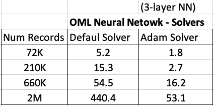
For me on my Oracle 20c Preview Database, this takes 1.8 seconds to run and create the neural network model ob a data set of 72,000 records.
Using the default solver, the model is created in 5.2 seconds. With using a small data set of 72,000 records, we can see the impact of using an Adam Solver for creating a neural network model.
These timings and the timings shown below (in seconds) are based on the Oracle 20c Preview Database, using a minimum VM sizing and specification available.
RandomForest Machine Learning – Oracle Machine Learning (OML)
Oracle Machine Learning has 30+ different machine learning algorithms built into the database. This means you can use SQL to create machine learning models and then use these models to score or label new data stored in the database or as the data is being created dynamically in the applications.
One of the most commonly used machine learning algorithms, over the past few years, is can RandomForest. This post will take a closer look at this algorithm and how you can build & use a RandomForest model.
Random Forest is known as an ensemble machine learning technique that involves the creation of hundreds of decision tree models. These hundreds of models are used to label or score new data by evaluating each of the decision trees and then determining the outcome based on the majority result from all the decision trees. Just like in the game show. The combining of a number of different ways of making a decision can result in a more accurate result or prediction.
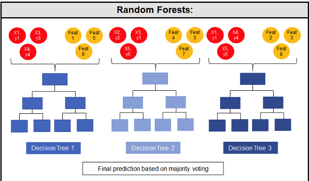
Random Forest models can be used for classification and regression types of problems, which form the majority of machine learning systems and solutions. For classification problems, this is where the target variable has either a binary value or a small number of defined values. For classification problems the Random Forest model will evaluate the predicted value for each of the decision trees in the model. The final predicted outcome will be the majority vote for all the decision trees. For regression problems the predicted value is numeric and on some range or scale. For example, we might want to predict a customer’s lifetime value (LTV), or the potential value of an insurance claim, etc. With Random Forest, each decision tree will make a prediction of this numeric value. The algorithm will then average these values for the final predicted outcome.
Under the hood, Random Forest is a collection of decision trees. Although decision trees are a popular algorithm for machine learning, they can have a tendency to over fit the model. This can lead higher than expected errors when predicting unseen data. It also gives just one possible way of representing the data and being able to derive a possible predicted outcome.
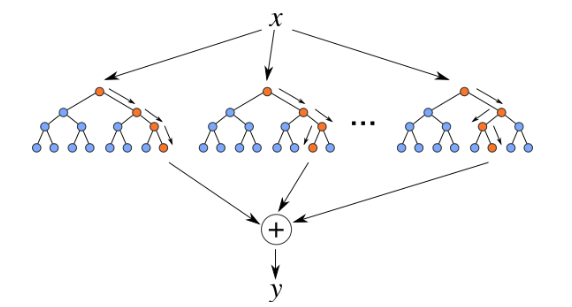 Random Forest on the other hand relies of the predicted outcomes from many different decision trees, each of which is built in a slightly different way. It is an ensemble technique that combines the predicted outcomes from each decision tree to give one answer. Typically, the number of trees created by the Random Forest algorithm is defined by a parameter setting, and in most languages this can default to 100+ or 200+ trees.
The Random Forest algorithm has three main features:
- It uses a method called bagging to create different subsets of the original training data
- It will randomly section different subsets of the features/attributes and build the decision tree based on this subset
- By creating many different decision trees, based on different subsets of the training data and different subsets of the features, it will increase the probability of capturing all possible ways of modeling the data
For each decision tree produced, the algorithm will use a measure, such as the Gini Index, to select the attributes to split on at each node of the decision tree.
To create a RandomForest model using Oracle Data Mining, you will follow the same process as with any of the other algorithms, the core of these are:
- define the parameter settings
- create the model
- score/label new data
Let’s start with the first step, defining the parameters. As with all the classification algorithms the same or similar parameters are set. With RandomForest we can set an additional parameter which tells the algorithm how many decision trees to create as part of the model. By default, 20 decision trees will be created. But if you want to change this number you can use the RFOR_NUM_TREES parameter. Remember the larger the value the longer it will take to create the model. But will have better accuracy. On the other hand with a small number of trees the quicker the model build will be, but might night be as accurate. This is something you will need to explore and determine. In the following example I change the number of trees to created to ten.
CREATE TABLE BANKING_RF_SETTINGS (
    SETTING_NAME VARCHAR2(50),
    SETTING_VALUE VARCHAR2(50)
);

BEGIN
  DELETE FROM BANKING_RF_SETTINGS;

  INSERT INTO banking_RF_settings (setting_name, setting_value)
  VALUES (dbms_data_mining.algo_name, dbms_data_mining.algo_random_forest);

  INSERT INTO banking_RF_settings (setting_name, setting_value)
  VALUES (dbms_data_mining.prep_auto, dbms_data_mining.prep_auto_on);

  INSERT INTO banking_RF_settings (setting_name, setting_value)
  VALUES (dbms_data_mining.RFOR_NUM_TREES, 10);

  COMMIT;
END;
Other default parameters used include, for creating each decision tree, use random 50% selection of columns and 50% sample of training data.
Now for step 2, create the model.
DECLARE
   v_start_time  TIMESTAMP;
BEGIN
   DBMS_DATA_MINING.DROP_MODEL('BANKING_RF_72K_1');

   v_start_time := current_timestamp;

   DBMS_DATA_MINING.CREATE_MODEL(
      model_name          => 'BANKING_RF_72K_1',
      mining_function     => dbms_data_mining.classification,
      data_table_name     => 'BANKING_72K',
      case_id_column_name => 'ID',
      target_column_name  => 'TARGET',
      settings_table_name => 'BANKING_RF_SETTINGS');

   dbms_output.put_line('Time take to create model = ' || to_char(extract(second from (current_timestamp-v_start_time))) || ' seconds.');
END;
The above code measures how long it takes to create the model.
I’ve run this same parameters and create models for different training data set sizes. I’ve also changed the number of decision trees to create. The following table shows the timings.
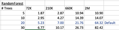
You can see it took 5.23 seconds to create a RandomForest model using the default settings for a data set of 72K records. This increase to just over one minute for a data set of 2 million records. Yo can also see the effect of reducing the number of decision trees on how long it takes the create model to run.
For step 3, on using the model on new data, this is just the same as with any of the classification models. Here is an example:
SELECT cust_id, target,
       prediction(BANKING_RF_72K_1 USING *)  predicted_value,
       prediction_probability(BANKING_RF_72K_1 USING *) probability
FROM   bank_test_v;
That’s it. That’s all there is to creating a RandomForest machine learning model using Oracle Machine Learning.
It’s quick and easy 🙂
MSET (Multivariate State Estimation Technique) in Oracle 20c
Updated: Changed 20c to Oracle 21c, as Oracle 20c Database never really existed 🙂
Oracle 21c Database comes with some new in-database Machine Learning algorithms.

The short name for one of these is called MSET or Multivariate State Estimation Technique. That’s the simple short name. The more complete name is Multivariate State Estimation Technique – Sequential Probability Ratio Test. That is a long name, and the reason is it consists of two algorithms. The first part looks at creating a model of the training data, and the second part looks at how new data is statistical different to the training data.
What are the use cases for this algorithm? This algorithm can be used for anomaly detection.
Anomaly Detection, using algorithms, is able identifying unexpected items or events in data that differ to the norm. It can be easy to perform some simple calculations and graphics to examine and present data to see if there are any patterns in the data set. When the data sets grow it is difficult for humans to identify anomalies and we need the help of algorithms.
The images shown here are easy to analyze to spot the anomalies and it can be relatively easy to build some automated processing to identify these. Most of these solutions can be considered AI (Artificial Intelligence) solutions as they mimic human behaviors to identify the anomalies, and these example don’t need deep learning, neural networks or anything like that.
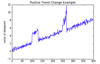
Other types of anomalies can be easily spotted in charts or graphics, such as the chart below.
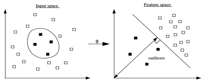 There are many different algorithms available for anomaly detection, and the Oracle Database already has an algorithm called the One-Class Support Vector Machine. This is a variant of the main Support Vector Machine (SVD) algorithm, which maps or transforms the data, using a Kernel function, into space such that the data belonging to the class values are transformed by different amounts. This creates a Hyperplane between the mapped/transformed values and hopefully gives a large margin between the mapped/transformed points. This is what makes SVD very accurate, although it does have some scaling limitations. For a One-Class SVD, a similar process is followed. The aim is for anomalous data to be mapped differently to common or non-anomalous data, as shown in the following diagram.
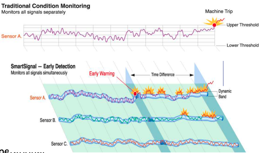
Getting back to the MSET algorithm. Remember it is a 2-part algorithm abbreviated to MSET. The first part is a non-linear, nonparametric anomaly detection algorithm that calibrates the expected behavior of a system based on historical data from the normal sequence of monitored signals. Using data in time series format (DATE, Value) the training data set contains data consisting of “normal” behavior of the data. The algorithm creates a model to represent this “normal”/stationary data/behavior. The second part of the algorithm compares new or live data and calculates the differences between the estimated and actual signal values (residuals). It uses Sequential Probability Ratio Test (SPRT) calculations to determine whether any of the signals have become degraded. As you can imagine the creation of the training data set is vital and may consist of many iterations before determining the optimal training data set to use.
MSET has its origins in computer hardware failures monitoring. Sun Microsystems have been were using it back in the late 1990’s-early 2000’s to monitor and detect for component failures in their servers. Since then MSET has been widely used in power generation plants, airplanes, space travel, Disney uses it for equipment failures, and in more recent times has been extensively used in IOT environments with the anomaly detection focused on signal anomalies.
How does MSET work in Oracle 21c?
An important point to note before we start is, you can use MSET on your typical business data and other data stored in the database. It isn’t just for sensor, IOT, etc data mentioned above and can be used in many different business scenarios.
The first step you need to do is to create the time series data. This can be easily done using a view, but a Very important component is the Time attribute needs to be a DATE format. Additional attributes can be numeric data and these will be used as input to the algorithm for model creation.
-- Create training data set for MSET
CREATE OR REPLACE VIEW mset_train_data
AS SELECT time_id,
          sum(quantity_sold) quantity,
          sum(amount_sold) amount
FROM (SELECT * FROM sh.sales WHERE time_id <= '30-DEC-99’)
GROUP BY time_id
ORDER BY time_id;
The example code above uses the SH schema data, and aggregates the data based on the TIME_ID attribute. This attribute is a DATE data type. The second import part of preparing and formatting the data is Ordering of the data. The ORDER BY is necessary to ensure the data is fed into or processed by the algorithm in the correct time series order.
The next step involves defining the parameters/hyper-parameters for the algorithm. All algorithms come with a set of default values, and in most cases these are suffice for your needs. In that case, you only need to define the Algorithm Name and to turn on Automatic Data Preparation. The following example illustrates this and also includes examples of setting some of the typical parameters for the algorithm.
BEGIN
  DELETE FROM mset_settings;

  -- Select MSET-SPRT as the algorithm
  INSERT  INTO mset_sh_settings (setting_name, setting_value)
  VALUES(dbms_data_mining.algo_name, dbms_data_mining.algo_mset_sprt);

  -- Turn on automatic data preparation
  INSERT INTO mset_sh_settings (setting_name, setting_value)
  VALUES(dbms_data_mining.prep_auto, dbms_data_mining.prep_auto_on);

  -- Set alert count
  INSERT INTO mset_sh_settings (setting_name, setting_value)
  VALUES(dbms_data_mining.MSET_ALERT_COUNT, 3);

  -- Set alert window
  INSERT INTO mset_sh_settings (setting_name, setting_value)
  VALUES(dbms_data_mining.MSET_ALERT_WINDOW, 5);

  -- Set alpha
  INSERT INTO mset_sh_settings (setting_name, setting_value)
  VALUES(dbms_data_mining.MSET_ALPHA_PROB, 0.1);

  COMMIT;
END;
To create the MSET model using the MST_TRAIN_DATA view created above, we can run:
BEGIN
--   DBMS_DATA_MINING.DROP_MODEL(MSET_MODEL');

   DBMS_DATA_MINING.CREATE_MODEL (
      model_name          => 'MSET_MODEL',
      mining_function     => dbms_data_mining.classification,
      data_table_name     => 'MSET_TRAIN_DATA',
      case_id_column_name => 'TIME_ID',
      target_column_name  => '',
      settings_table_name => 'MSET_SETTINGS');
END;
The SELECT statement below is an example of how to call and run the MSET model to label the data to find anomalies. The PREDICTION function will return a values of 0 (zero) or 1 (one) to indicate the predicted values. If the predicted values is 0 (zero) the MSET model has predicted the input record to be anomalous, where as a predicted values of 1 (one) indicates the value is typical. This can be used to filter out the records/data you will want to investigate in more detail.
-- display all dates with Anomalies
SELECT time_id, pred
FROM (SELECT time_id, prediction(mset_sh_model using *) over (ORDER BY time_id) pred
      FROM mset_test_data)
WHERE pred = 0;
Storing and processing Unicode characters in Oracle
Unicode is a computing industry standard for the consistent encoding, representation, and handling of text expressed in most of the world’s writing systems (Wikipedia). The standard is maintained by the Unicode Consortium, and contains over 137,994 characters (137,766 graphic characters, 163 format characters and 65 control characters).
The NVARCHAR2 is Unicode data type that can store Unicode characters in an Oracle Database. The character set of the NVARCHAR2 is national character set specified at the database creation time. Use the following to determine the national character set for your database.
SELECT *
FROM nls_database_parameters
WHERE PARAMETER = 'NLS_NCHAR_CHARACTERSET';
For my database I’m using an Oracle Autonomous Database. This query returns the character set AL16UTF16. This character set encodes Unicode data in the UTF-16 encoding and uses 2 bytes to store a character.
When creating an attribute with this data type, the size value (max 4000) determines the number of characters allowed. The actual size of the attribute will be double.
Let’s setup some data to test this data type.
CREATE TABLE demo_nvarchar2 (
   attribute_name NVARCHAR2(100));

INSERT INTO demo_nvarchar2
VALUES ('This is a test for nvarchar2');
The string is 28 characters long. We can use the DUMP function to see the details of what is actually stored.
SELECT attribute_name, DUMP(attribute_name,1016)
FROM demo_nvarchar2;
The DUMP function returns a VARCHAR2 value that contains the datatype code, the length in bytes, and the internal representation of a value.

You can see the difference in the storage size of the NVARCHAR2 and the VARCHAR2 attributes.
Valid values for the return_format are 8, 10, 16, 17, 1008, 1010, 1016 and 1017. These values are assigned the following meanings:
8 – octal notation
10 – decimal notation
16 – hexadecimal notation
17 – single characters
1008 – octal notation with the character set name
1010 – decimal notation with the character set name
1016 – hexadecimal notation with the character set name
1017 – single characters with the character set name
The returned value from the DUMP function gives the internal data type representation. The following table lists the various codes and their description.
| Code | Data Type |
|---|---|
| 1 | VARCHAR2(size [BYTE | CHAR]) |
| 1 | NVARCHAR2(size) |
| 2 | NUMBER[(precision [, scale]]) |
| 8 | LONG |
| 12 | DATE |
| 21 | BINARY_FLOAT |
| 22 | BINARY_DOUBLE |
| 23 | RAW(size) |
| 24 | LONG RAW |
| 69 | ROWID |
| 96 | CHAR [(size [BYTE | CHAR])] |
| 96 | NCHAR[(size)] |
| 112 | CLOB |
| 112 | NCLOB |
| 113 | BLOB |
| 114 | BFILE |
| 180 | TIMESTAMP [(fractional_seconds)] |
| 181 | TIMESTAMP [(fractional_seconds)] WITH TIME ZONE |
| 182 | INTERVAL YEAR [(year_precision)] TO MONTH |
| 183 | INTERVAL DAY [(day_precision)] TO SECOND[(fractional_seconds)] |
| 208 | UROWID [(size)] |
| 231 | TIMESTAMP [(fractional_seconds)] WITH LOCAL TIMEZONE |
Reading Data from Oracle Table into Python Pandas – How long & Different arraysize
Here are some results from a little testing I recent did on extracting data from an Oracle database and what effect the arraysize makes and which method might be the quickest.
The arraysize determines how many records will be retrieved in each each batch. When a query is issued to the database, the results are returned to the calling programme in batches of a certain size. Depending on the nature of the application and the number of records being retrieved, will determine the arraysize value. The value of this can have a dramatic effect on your query and application response times. Sometimes a small value works very well but sometimes you might need a larger value.
My test involved using an Oracle Database Cloud instance, using Python and the following values for the arraysize.
arraysize = (5, 50, 500, 1000, 2000, 3000, 4000, 5000)
The first test was to see what effect these arraysizes have on retrieving all the data from a table. The in question has 73,668 records. So not a large table. The test loops through this list of values and fetches all the data, using the fetchall function (part of cx_Oracle), and then displays the time taken to retrieve the results.
# import the Oracle Python library
import cx_Oracle
import datetime
import pandas as pd
import numpy as np

# setting display width for outputs in PyCharm
desired_width = 280
pd.set_option('display.width', desired_width)
np.set_printoptions(linewidth=desired_width)
pd.set_option('display.max_columns',30)

# define the login details
p_username = "************"
p_password = "************"
p_host = "************"
p_service = "************"
p_port = "1521"

print('--------------------------------------------------------------------------')
print(' Testing the time to extract data from an Oracle Database.')
print('    using different approaches.')
print('---')
# create the connection
con = cx_Oracle.connect(user=p_username, password=p_password, dsn=p_host+"/"+p_service+":"+p_port)

print('')
print(' Test 1: Extracting data using Cursor for different Array sizes')
print('    Array Size = 5, 50, 500, 1000, 2000, 3000, 4000, 5000')
print('')
print('   Starting test at : ', datetime.datetime.now())

beginTime = datetime.datetime.now()
cur_array_size = (5, 50, 500, 1000, 2000, 3000, 4000, 5000)
sql = 'select * from banking_marketing_data_balance_v'

for size in cur_array_size:
    startTime = datetime.datetime.now()
    cur = con.cursor()
    cur.arraysize = size
    results = cur.execute(sql).fetchall()
    print('      Time taken : array size = ', size, ' = ', datetime.datetime.now()-startTime, ' seconds,  num of records = ', len(results))
    cur.close()

print('')
print('   Test 1: Time take = ', datetime.datetime.now()-beginTime)
print('')
And here are the results from this first test.
Starting test at :  2018-11-14 15:51:15.530002
      Time taken : array size =  5  =  0:36:31.855690  seconds,  num of records =  73668
      Time taken : array size =  50  =  0:05:32.444967  seconds,  num of records =  73668
      Time taken : array size =  500  =  0:00:40.757931  seconds,  num of records =  73668
      Time taken : array size =  1000  =  0:00:14.306910  seconds,  num of records =  73668
      Time taken : array size =  2000  =  0:00:10.182356  seconds,  num of records =  73668
      Time taken : array size =  3000  =  0:00:20.894687  seconds,  num of records =  73668
      Time taken : array size =  4000  =  0:00:07.843796  seconds,  num of records =  73668
      Time taken : array size =  5000  =  0:00:06.242697  seconds,  num of records =  73668
As you can see the variation in the results.
You may get different performance results based on your location, network connectivity and proximity of the database. I was at home (Ireland) using wifi and my database was located somewhere in USA. I ran the rest a number of times and the timings varied by +/- 15%, which is a lot!
When the data is retrieved in this manner you can process the data set in the returned results set. Or what is more traditional you will want to work with the data set as a panda. The next two test look at a couple of methods of querying the data and storing the result sets in a panda.
For these two test, I’ll set the arraysize = 3000. Let’s see what happens.
For the second test I’ll again use the fetchall() function to retrieve the data set. From that I extract the names of the columns and then create a panda combining the results data set and the column names.
startTime = datetime.datetime.now()
print('   Starting test at : ', startTime)
cur = con.cursor()
cur.arraysize = cur_array_size
results = cur.execute(sql).fetchall()
print('   Fetched ', len(results), ' in ', datetime.datetime.now()-startTime, ' seconds at ', datetime.datetime.now())
startTime2 = datetime.datetime.now()
col_names = []
for i in range(0, len(cur.description)):
    col_names.append(cur.description[i][0])

print('      Fetched data & Created the list of Column names in ', datetime.datetime.now()-startTime, ' seconds at ', datetime.datetime.now())
The results from this are.
      Fetched  73668  in  0:00:07.778850  seconds at  2018-11-14 16:35:07.840910
      Fetched data & Created the list of Column names in  0:00:07.779043  seconds at  2018-11-14 16:35:07.841093
      Finished creating Dataframe in  0:00:07.975074  seconds at  2018-11-14 16:35:08.037134

Test 2: Total Time take =  0:00:07.975614
Now that was quick. Fetching the data set in just over 7.7788 seconds. Creating the column names as fractions of a millisecond, and then the final creation of the panda took approx 0.13 seconds.
For the third these I used the pandas library function called read_sql(). This function takes two inputs. The first is the query to be processed and the second the name of the database connection.
print(' Test 3: Test timing for read_sql into a dataframe')
cur_array_size = 3000
print('   will use arraysize = ', cur_array_size)
print('')
startTime = datetime.datetime.now()
print('   Starting test at : ', startTime)

df2 = pd.read_sql(sql, con)

print('      Finished creating Dataframe in ', datetime.datetime.now()-startTime, ' seconds at ', datetime.datetime.now())
# close the connection at end of experiments
con.close()
and the results from this are.
   Test 3: Test timing for read_sql into a dataframe will use arraysize =  3000

   Starting test at :  2018-11-14 16:35:08.095189
      Finished creating Dataframe in  0:02:03.200411  seconds at  2018-11-14 16:37:11.295611
You can see that it took just over 2 minutes to create the panda data frame using the read_sql() function, compared to just under 8 seconds using the previous method.
It is important to test the various options for processing your data and find the one that works best in your environment. As with most languages there can be many ways to do the same thing. The challenge is to work out which one you should use.
OUG Ireland 2017 Presentation
Here are the slides from my presentation at OUG Ireland 2017. All about running R using SQL.
- ← Previous
- 1
- 2
- 3
- Next →

You must be logged in to post a comment.